1 Introduction
Scale interactions have been extensively addressed in canonical zero-pressure-gradient turbulent boundary layer flows over a wide range of smooth and rough surfaces, or densely distributed roughness elements (see Warhaft Reference Warhaft2002; Poggi et al.
Reference Poggi, Porporato, Ridolfi, Albertson and Katul2004; Hutchins & Marusic Reference Hutchins and Marusic2007a
; Guala, Metzger & McKeon Reference Guala, Metzger and McKeon2011, among others). This includes the smooth-wall turbulent boundary layer where the largest scales such as very-large-scale motions (VLSMs) and superstructures (Kim & Adrian Reference Kim and Adrian1999; Guala, Hommema & Adrian Reference Guala, Hommema and Adrian2006; Hutchins & Marusic Reference Hutchins and Marusic2007b
; Smits, McKeon & Marusic Reference Smits, McKeon and Marusic2011) have been observed to interact with the small-scale turbulence populating the near-wall region (Hutchins & Marusic Reference Hutchins and Marusic2007a
; Mathis, Hutchins & Marusic Reference Mathis, Hutchins and Marusic2009; Marusic, Mathis & Hutchins Reference Marusic, Mathis and Hutchins2010). The result of such interactions has been quantified in terms of amplitude modulation, anisotropy and inhomogeneity of the dissipative scales, manifested through an increased intermittency (Laval, Dubrulle & Nazarenko Reference Laval, Dubrulle and Nazarenko2001; Mininni, Alexakis & Pouquet Reference Mininni, Alexakis and Pouquet2006; Guala, Metzger & McKeon Reference Guala, Metzger and McKeon2010; de Silva et al.
Reference de Silva, Marusic, Woodcock and Meneveau2015), in particular, near the wall. In such a region, strong coupling between widely separated scales in the spectral domain results in a ‘non-local’ energy transfer (Yeung, Brasseur & Wang Reference Yeung, Brasseur and Wang1995; Warhaft Reference Warhaft2002; Poggi et al.
Reference Poggi, Porporato, Ridolfi, Albertson and Katul2004; Mininni et al.
Reference Mininni, Alexakis and Pouquet2006; Keylock, Singh & Foufoula-Georgiou Reference Keylock, Singh and Foufoula-Georgiou2013; Keylock et al.
Reference Keylock, Singh, Venditti and Foufoula-Georgiou2014; Singh, Howard & Guala Reference Singh, Howard and Guala2014; de Silva et al.
Reference de Silva, Marusic, Woodcock and Meneveau2015). This mechanism is different from the ‘local’ energy transfer between neighbouring scales in a Fourier sense, hypothesized in the Kolmogorov (Reference Kolmogorov1941) model of energy cascade, under the small-scale isotropy assumption. It is argued that, when turbulence does not have the time/space to dissipate energy at the rate required by the energy-containing eddies, non-uniform transfer of energy takes place from large to smaller scales, resulting in abrupt intense gradients in the velocity time series. These intense events are amplified in high-order structure function statistics causing a deviation from the Kolmogorov (Reference Kolmogorov1941) prediction (Menevau & Sreenivasan Reference Menevau and Sreenivasan1991; Benzi et al.
Reference Benzi, Ciliberto, Tripiccione, Baudet, Massaioli and Succi1993; Guala et al.
Reference Guala, Metzger and McKeon2010). In addition, the same rare, highly dissipative events are responsible for a positive skewness in the distribution of the streamwise velocity increments, pointing at a close link between intermittency and anisotropy (Warhaft Reference Warhaft2002; Singh et al.
Reference Singh, Foufoula-Georgiou, Porté-Agel and Wilcock2012, Reference Singh, Howard and Guala2014). This phenomenological interpretation fits well with the wall structure organization at high Reynolds number inferred by Morrison (Reference Morrison2007) and Guala et al. (Reference Guala, Metzger and McKeon2011), suggesting that large outer-scale motions and near-wall inner scales approaching the dissipative range strongly interact, favouring rare dissipative events at the wall (see also Jimenez Reference Jimenez2000; Mazellier & Vassilicos Reference Mazellier and Vassilicos2008). From a historical perspective (for details, see Frisch Reference Frisch1995), strong scale interactions are inferred to be driven by inhomogeneity and anisotropy at the scale of the turbulent kinetic energy production, which, in this specific context, are identified as the large-scale structures of the turbulent boundary layer. Such inhomogeneities at the large scales represent the main criticism to the Kolmogorov (Reference Kolmogorov1941) universal assumptions (see e.g. Kraichnan Reference Kraichnan1974), and the phenomenological interpretation of the observed near-wall intermittency. Despite decades of ongoing research, the connection between the structure of wall turbulence, near-wall anisotropy and intermittency that leads to nonlinear interactions between large- and small-scale flow structures remains poorly understood. We hope to shed some light with this contribution, originating from an unanticipated experimental observation in Singh et al. (Reference Singh, Howard and Guala2014). In such previous work, devoted to the study of the structure of the flow in the wake of a model wind turbine, we evidenced an anomaly, in the form of a hump, in the asymmetry of the distribution of the, scale-dependent, increments of the streamwise velocity. Surprisingly, the anomaly appeared not in the turbine wake flow, but rather in the baseline flow, i.e. the zero-pressure-gradient turbulent boundary layer achieved in the St. Anthony Falls Laboratory (SAFL) atmospheric wind tunnel. The observed hump was located in the frequency and amplitude ranges where Basu et al. (Reference Basu, Foufoula-Georgiou, Lashermes and Arnéodo2007) observed, and barely acknowledged, a similar feature (using the Kunkel & Marusic (Reference Kunkel and Marusic2006) data in the atmospheric surface layer at Surface Layer Turbulence and Environmental Science Test (SLTEST) facility). Singh et al. (Reference Singh, Howard and Guala2014) interpreted the anomaly as a peak in the scale coupling activity, occurring in a range of scales between the Kolmogorov scale and the integral time scale (
 $ITS$
), in fact covering nearly the entire inertial range.
In this work, in addition to SAFL wind tunnel measurements, we use the SLTEST measurements published in Metzger, McKeon & Holmes (Reference Metzger, McKeon and Holmes2007) and Guala et al. (Reference Guala, Metzger and McKeon2011) to confirm the occurrence, and investigate the scaling, of the asymmetry hump, aiming to provide a more in-depth interpretation of such anomaly, inferred here to be a universal, genuine, feature of turbulent boundary layer flows. The added benefit of this specific high-Reynolds-number dataset lies in the multi-hot-wire simultaneous acquisition providing (i) high vertical resolution (via 29 sensors logarithmically spaced up to 5 m above the ground level), (ii) statistical convergence of the mean and the root-mean-square (r.m.s.) streamwise velocities (Guala et al.
Reference Guala, Metzger and McKeon2011), and (iii) strictly neutral thermal stability conditions (
 $z/L<0.01$
(Metzger et al.
Reference Metzger, McKeon and Holmes2007), where
 $z$
indicates the measurement height and
 $L$
the Monin Obhukov length). The comparative analysis across the two datasets ensures that the wall-normal scaling arguments are independent of the Reynolds number, which strengthens the importance of the SLTEST data to avoid scaling ambiguities: high Reynolds number
 $u_{{\it\tau}}{\it\delta}/{\it\nu}$
implies that the outer scale (
 ${\it\delta}$
) and the inner, viscous scale (
 ${\it\nu}/u_{{\it\tau}}$
) are well separated (here
 $u_{{\it\tau}}$
is the shear velocity,
 ${\it\delta}$
is the boundary layer height and
 ${\it\nu}$
is the kinematic viscosity). The asymmetry index provides the additional benefit to be a compact, scale-dependent, height-dependent variable that can be used also as a probe to infer how the structural population of turbulent boundary layer flows evolve with the Reynolds number.
The paper is structured as follows. In the following section we briefly outline the two experimental set-ups and the data used in this study. Section 3 presents major results based on magnitude cumulant analysis and asymmetry index, providing inner and outer scaling arguments for the two different Reynolds-number flows studied here. Finally, the summary and conclusions drawn are presented in § 4.
2 Brief description of the datasets analysed
We present here two datasets, from wind tunnel (WT) and atmospheric surface layer SLTEST (SLT), each comprising a profile of instantaneous streamwise velocity time series sampled at high resolution with hot-wire probes. Both datasets were obtained in nearly smooth zero-pressure-gradient turbulent boundary layer flows at very different Reynolds numbers,
 $Re_{{\it\tau}}=u_{{\it\tau}}{\it\delta}/{\it\nu}\simeq 6.7\times 10^{5}$
(SLT) and
 $1.3\times 10^{4}$
(WT). The SLT data were captured at the SLTEST site in the Great Salt Lake Flats in Utah, a renowned field for near-wall atmospheric boundary layer studies (Metzger & Klewicki Reference Metzger and Klewicki2001; Smits et al.
Reference Smits, McKeon and Marusic2011, and references therein). The current dataset was acquired in May 2005 and extensively presented and discussed in Metzger et al. (Reference Metzger, McKeon and Holmes2007) and Guala et al. (Reference Guala, Metzger and McKeon2010, Reference Guala, Metzger and McKeon2011). A total of 29 logarithmically spaced hot-wire probes were used to sample at 5 kHz the streamwise velocity up to a height of
 ${\approx}$
5 m in the atmospheric surface layer. The particularly favourable conditions (neat, monitored transition between the convective and the stable stratified boundary layer with
 $|z/L|<0.01$
, persistence in the wind magnitude and direction) allowed this dataset to be representative of the canonical high-Reynolds-number turbulent boundary layer flow. The WT data were obtained in the SAFL atmospheric, temperature-controlled, wind tunnel (Carper & Porté-Agel Reference Carper and Porté-Agel2008; Chamorro & Porté-Agel Reference Chamorro and Porté-Agel2009; Singh et al.
Reference Singh, Howard and Guala2014; Howard et al.
Reference Howard, Hu, Chamorro and Guala2015a
,Reference Howard, Singh, Sotiropoulos and Guala
b
). The main test section in the wind tunnel is 16 m long, 1.7 m wide and 1.7 m high, with a picket fence trip allowing the boundary layer to grow up to approximately
 ${\it\delta}\simeq 0.6$
m in the available 16 m fetch. The floor and air temperatures were controlled separately, allowing the implementation of desired thermal stratification conditions in the boundary layer or a constant temperature profile (neutral conditions), as in this experiment. The WT data were acquired for baseline flow characterization in the Singh et al. (Reference Singh, Howard and Guala2014) study on wind turbine model wakes. A cross-wire anemometer was used to measure instantaneous streamwise and vertical flow velocities at a frequency of 10 kHz, for a total acquisition time of 300 s (
 $3\times 10^{6}$
points) per vertical location. Measurement points were spaced 0.01 m in the vertical direction from 0.004 m to 0.7 m.
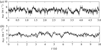
Figure 1 shows the typical time series of streamwise velocities for the WT (figure 1
a) and for the SLT (figure 1
b) collected at a normalized vertical distance of
 $z^{+}\sim 1500$
(
 $z^{+}=zu_{{\it\tau}}/{\it\nu}$
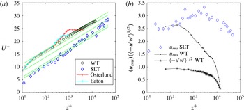
). Figure 2(a) shows the mean velocity profile for the WT (circles) and the SLT (diamonds) datasets, while table 1 lists the main characteristics of the two boundary layer flows. The streamwise r.m.s. velocities, normalized by
 $u_{{\it\tau}}$
for both WT and SLT, along with Reynolds stress for WT can be seen in figure 2(b). As exhaustively discussed in Metzger et al. (Reference Metzger, McKeon and Holmes2007) and Guala et al. (Reference Guala, Metzger and McKeon2011), we acknowledge that the SLT mean velocity profile manifests a weak contamination from roughness effects, with a sand-equivalent roughness estimated as
 $k_{s}^{+}\approx 25$
; this implies that results obtained at
 $z^{+}<3k_{s}^{+}\sim 75$
must be taken with some caution. Also note that the apparent WT–SLT discrepancy in the streamwise velocity turbulent intensity profile
 $u_{rms}(z^{+})$
for
 $z^{+}>3\times 10^{2}$
is a clear effect of the increased Reynolds number (Metzger et al.
Reference Metzger, McKeon and Holmes2007).
Time series of streamwise flow velocities sampled at a frequency of 10 000 Hz for the case of wind tunnel WT (a) and at a frequency of 5000 Hz for the case of SLTEST SLT (b). Measurements were acquired at comparable heights in wall units,
 $z^{+}=1587$
(WT) and
 $z^{+}=1464$
(SLT).

Mean (a) and fluctuating (b) streamwise velocity statistics for the WT and SLT datasets, normalized with the shear velocity
 $u_{{\it\tau}}$
. Inclined lines in (a) indicate the logarithmic mean velocity profile for the smooth case and for increasing roughness
 $k_{s}^{+}=5,~10,~25,~35$
(for reference). The
 $+$
symbols refer to measurements from De Graaf & Eaton (Reference De Graaff and Eaton2000) at
 $Re_{{\it\tau}}=1430$
and Osterlund (Reference Osterlund1999) at
 $Re_{{\it\tau}}=2530$
. Subscript rms in (b) represents root-mean-square velocity.

Mean flow statistics for the wind tunnel (WT) and atmospheric surface layer (SLT) datasets:
 $T_{total}$
indicates the total sampling time at each measurement location, while
 $N_{p}$
is the number of probe locations in the vertical direction. The ranges of heights covered in the two datasets are reported in viscous (
 $z^{+}$
) and outer units (
 $z/{\it\delta}$
).

3 Results and discussion
3.1 Magnitude cumulant analysis: a measure of intermittency
Spatial or temporal series of velocity fluctuations in turbulent flows are typically decomposed into Fourier modes to compute the power spectral density that describes the energetic contribution of eddies of different sizes, or, in statistical terms, identifies scale-dependent variations of the second-order moment, or variance (Singh, Porté-Agel & Foufoula-Georgiou Reference Singh, Porté-Agel and Foufoula-Georgiou2010; Singh et al.
Reference Singh, Howard and Guala2014). In addition, the power spectrum provides all the necessary information for re-creating a representative turbulent velocity time series in the case when the velocity increments are Gaussian-distributed over a range of scales (Singh et al.
Reference Singh, Lanzoni, Wilcock and Foufoula-Georgiou2011, Reference Singh, Foufoula-Georgiou, Porté-Agel and Wilcock2012); the velocity increments are defined here as
 ${\rm\Delta}u(t,a)=u(t+a)-u(t)$
as a function of the separation time scale
 $a$
. However, the distribution of the velocity increments in a turbulent signal usually shows significant deviation from the Gaussian distribution at smaller scales, i.e. for values of
 $a$
approaching the Kolmogorov time scale
 ${\it\tau}_{k}$
(see e.g. Malecot et al.
Reference Malecot, Auriault, Kahalerras, Gagne, Chanal, Chabaud and Castaing2000; Ruiz-Chavarria et al.
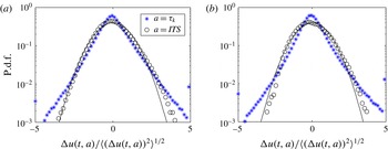
Reference Ruiz-Chavarria, Ciliberto, Baudet and Lévêqueb2000). This can also be observed in the probability distribution function (p.d.f.) of velocity increments for WT (figure 3
a) and SLT (figure 3
b), suggesting (i) a multiscaling type of behaviour of turbulent velocity fluctuations, and (ii) that higher order statistical moments are required for reconstructing the original velocity signal. Note that the Kolmogorov time scale is defined here as
 ${\it\tau}_{k}={\it\eta}/U$
, where
 ${\it\eta}=({\it\nu}^{3}/{\it\epsilon})^{1/4}$
is the Kolmogorov length scale,
 ${\it\epsilon}$
is the average rate of dissipation of turbulent kinetic energy,
 ${\it\nu}$
is the kinematic viscosity and
 $U$
is the average convective velocity. This is an advective form of the Kolmogorov time scale, which is different from the Kolmogorov time scale
 ${\it\tau}=({\it\nu}/{\it\epsilon})^{1/2}$
used in homogeneous turbulence and inadequate when the convective velocity is much larger than the Kolmogorov velocity. The
 $ITS$
is estimated using the integral of the autocorrelation function of the streamwise velocity.
Semilogarithmic p.d.f.s of the normalized form of the velocity increments
 ${\rm\Delta}u(t,a)=u(t+a)-u(t)$
) for the scales
 $a={\it\tau}_{k}$
and
 $a=ITS$
for both WT (a) and SLT (b) datasets. The solid curve denotes the Gaussian distribution. P.d.f.s are shown for
 $z_{WT}^{+}=1587$
(a) and
 $z_{SLT}^{+}=1464$
(b).

While a large amount of work has been devoted to high-order structure function analysis (Menevau & Sreenivasan Reference Menevau and Sreenivasan1991; Toschi, Leveque & Ruiz-Chavarria Reference Toschi, Leveque and Ruiz-Chavarria2000; Venugopal et al.
Reference Venugopal, Roux, Foufoula-Georgiou and Arnéodo2006; Basu et al.
Reference Basu, Foufoula-Georgiou, Lashermes and Arnéodo2007; Kholmyansky, Moriconi & Tsinober Reference Kholmyansky, Moriconi and Tsinober2007; Singh et al.
Reference Singh, Fienberg, Jerolmack, Marr and Foufoula-Georgiou2009, Reference Singh, Lanzoni, Wilcock and Foufoula-Georgiou2011; Guala et al.
Reference Guala, Metzger and McKeon2010), an alternative method has been proposed in the form of the magnitude cumulant analysis, introduced by Delour, Muzy & Arnéodo (Reference Delour, Muzy and Arnéodo2001) – see also Malecot et al. (Reference Malecot, Auriault, Kahalerras, Gagne, Chanal, Chabaud and Castaing2000) and Chevillard et al. (Reference Chevillard, Roux, Leveque, Mordant, Pinton and Arneodo2005). This approach requires only the second-order magnitude cumulant to unravel the underlying intermittency in the turbulence structure of the velocity signal, under the assumption of log-normality in the increment distribution (see e.g. Delour et al.
Reference Delour, Muzy and Arnéodo2001; Chevillard et al.
Reference Chevillard, Roux, Leveque, Mordant, Pinton and Arneodo2005; Basu et al.
Reference Basu, Foufoula-Georgiou, Lashermes and Arnéodo2007; Singh et al.
Reference Singh, Howard and Guala2014). In general, for a random variable
 $X$
having a p.d.f.
 $F(x)$
, the moment generating function (also defined as the characteristic function) can be expressed as
 $$\begin{eqnarray}{\it\phi}_{p}(k)=\int _{-\infty }^{+\infty }\text{e}^{\text{i}kx}F(x)\,\text{d}x,\end{eqnarray}$$
which can be expanded in a Taylor’s series as the following and leading to
 $$\begin{eqnarray}{\it\phi}_{p}(k)=\langle \text{e}^{\text{i}kx}\rangle =\left\langle 1+\text{i}kx+\frac{(\text{i}kx)^{2}}{2!}+\frac{(\text{i}kx)^{3}}{3!}+\,\cdots \right\rangle =\mathop{\sum }_{n=0}^{\infty }M_{n}\frac{(\text{i}k)^{n}}{n!},\end{eqnarray}$$
where
 $M_{n}$
is the
 $n$
th-order moment of
 $X$
, represented as
 $$\begin{eqnarray}M_{n}=\int _{-\infty }^{+\infty }x^{n}F(x)\,\text{d}x,\quad n=0,1,2,\ldots .\end{eqnarray}$$
Analogously,
 $M_{n}$
can be estimated by the
 $n$
th-order derivative of
 ${\it\phi}_{p}(k)$
at
 $k=0$
. The cumulant generating function of
 $X$
can be accordingly defined as
 $$\begin{eqnarray}{\it\psi}_{p}(k)\equiv \ln {\it\phi}_{p}(k)=\ln \langle \text{e}^{\text{i}kx}\rangle ,\end{eqnarray}$$
while the cumulant
 $C_{n}$
of
 $X$
can be obtained from the
 $n$
th derivative of
 ${\it\psi}_{p}(k)$
. Moments and cumulants can be related as
 $$\begin{eqnarray}\displaystyle & C_{1}=M_{1}, & \displaystyle\end{eqnarray}$$
 $$\begin{eqnarray}\displaystyle & C_{2}=M_{2}-M_{1}^{2}, & \displaystyle\end{eqnarray}$$
 $$\begin{eqnarray}\displaystyle & C_{3}=M_{3}-3M_{2}M_{1}+2M_{1}^{3}, & \displaystyle\end{eqnarray}$$
 $$\begin{eqnarray}\displaystyle & C_{4}=M_{4}-4M_{3}M_{1}-3M_{2}^{2}+12M_{2}M_{1}^{2}-6M_{1}^{4}, & \displaystyle\end{eqnarray}$$
and so on.
If we substitute the variable
 $X$
with the velocity increment
 ${\rm\Delta}u$
separated by a given lag
 $a$
, the magnitude cumulant
 $C_{n}$
can be expressed as
 $$\begin{eqnarray}\langle |{\rm\Delta}_{a}u|^{q}\rangle =\exp \left(\mathop{\sum }_{n=1}^{\infty }C_{n}(a)\frac{q^{n}}{n!}\right),\end{eqnarray}$$
where
 $$\begin{eqnarray}\displaystyle & C_{1}=\langle \ln |{\rm\Delta}u|\rangle \sim c_{1}\ln (a), & \displaystyle\end{eqnarray}$$
 $$\begin{eqnarray}\displaystyle & C_{2}=\langle (\ln |{\rm\Delta}u|)^{2}\rangle -\langle \ln |{\rm\Delta}u|\rangle ^{2}\sim -c_{2}\ln (a), & \displaystyle\end{eqnarray}$$
 $$\begin{eqnarray}\displaystyle & C_{3}=\langle (\ln |{\rm\Delta}u|)^{3}\rangle -3\langle (\ln |{\rm\Delta}u|)^{2}\rangle \langle \ln |{\rm\Delta}u|\rangle +2\langle \ln |{\rm\Delta}u|\rangle ^{3}\sim c_{3}\ln (a). & \displaystyle\end{eqnarray}$$
Cumulants
 $C_{1}$
and
 $C_{2}$
are scale-dependent functions of the mean
 $\langle \ln |{\rm\Delta}u|\rangle$
and the variance
 $\langle (\ln |{\rm\Delta}u|)^{2}\rangle$
(for more details, see Malecot et al.
Reference Malecot, Auriault, Kahalerras, Gagne, Chanal, Chabaud and Castaing2000; Delour et al.
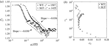
Reference Delour, Muzy and Arnéodo2001). Figure 4(a) shows the second-order cumulant
 $C_{2}$
as a function of scale
 $a$
normalized by the
 $ITS$
for both WT and SLT (see also Singh et al. (Reference Singh, Howard and Guala2014) for the plot of
 $C_{1}(a)$
, whose slope from log-linear regime represents the Hölder exponent
 $\langle h\rangle$
, for the WT dataset). The slope of the log-linear regime obtained from second-order cumulant
 $C_{2}(a)$
within the range of scales of interest (from Kolmogorov scale to integral time scale,
 ${\it\tau}_{k}<a<ITS$
), is used to define the intermittency coefficient
 $c_{2}$
;
 $c_{2}$
represents a compact, scale-independent, parameter describing the structure of each streamwise velocity increment time series, by providing a measure of the inhomogeneous temporal arrangement of its local abrupt fluctuations (Singh et al.
Reference Singh, Lanzoni, Wilcock and Foufoula-Georgiou2011, Reference Singh, Foufoula-Georgiou, Porté-Agel and Wilcock2012) and is not to be confused with the above-defined second-order cumulant
 $C_{2}$
notation.
Figure 4(b) shows the computed intermittency coefficient
 $c_{2}$
profiles for the WT and SLT cases, for the range of wall-normal distances
 $z^{+}$
explored here. It is noted that the estimated intermittency coefficients
 $c_{2}$
obtained from traditional high-order structure function analysis (not shown here for brevity) resulted in similar values as obtained from the magnitude cumulant analysis presented here. As can be seen from figure 4(b), the
 $c_{2}$
profiles for both WT and SLT are very similar and, in fact, overlap for a range of
 $z^{+}$
, particularly in the range
 $z^{+}\sim 70{-}10^{3}$
. For the lower
 $z^{+}$
, SLTEST data show an increase in
 $c_{2}$
with decreasing
 $z^{+}$
, suggesting an increase in the frequency and magnitude of the intense velocity gradients that may have resulted from increasing mean shear as
 $z^{+}$
decreases (see also Antonia, Orlandi & Romano Reference Antonia, Orlandi and Romano1998; Onorato, Camussi & Iuso Reference Onorato, Camussi and Iuso2000). Note that, in the case of a monofractal signal, where the shape of the increment distributions of the signal does not change with the scale
 $a$
, the intermittency coefficient
 $c_{2}$
is precisely
 $0$
. Also, note that the
 $c_{2}$
values in our study for both WT and SLT datasets are consistent with the
 $c_{2}$
observed in Basu et al. (Reference Basu, Foufoula-Georgiou, Lashermes and Arnéodo2007) for a similar dataset in the atmospheric surface layer.
(a) Second-order cumulant
 $C_{2}$
as a function of scale
 $a$
normalized by the
 $ITS$
and (b) vertical profile of intermittency coefficients (
 $c_{2}$
) as a function of vertical wall distance
 $z^{+}$
for the streamwise velocity for both WT (stars) and SLT (circles). Note that the intermittency coefficients
 $c_{2}$
shown in figure 4(b) are computed from the second-order cumulants
 $C_{2}$
(figure 4
a) for a range of scales, i.e. Kolmogorov scale
 ${\it\tau}_{k}$
to
 $ITS$
.

3.2 Scale-dependent asymmetry of the velocity increments
From figure 3 it was noticed that the p.d.f.s of the velocity increments, for varying time scale
 $a$
, are neither Gaussian nor symmetric, a combination that is inferred to point at multiplicative cascade processes and non-local scale interactions (Schertzer et al.
Reference Schertzer, Lovejoy, Schmitt, Chiguirinskaya and Marsan1997; Warhaft Reference Warhaft2002; Singh et al.
Reference Singh, Foufoula-Georgiou, Porté-Agel and Wilcock2012, Reference Singh, Howard and Guala2014). While non-Gaussianity is expressed through the intermittency coefficient
 $c_{2}$
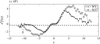
, the asymmetry in the distribution can be quantified using either the third or the fifth moment function (as in this study) of the velocity increments (see Warhaft Reference Warhaft2002). Results are provided in figure 5 for WT and SLT velocity time series at
 $z^{+}\sim 1500$
for the smallest scale separation
 $a={\it\tau}_{k}$
. The qualitative behaviour of the two curves directs attention towards a Reynolds-number-independent feature of the turbulent boundary layer, regarding the distribution and statistical weight of rare but intense dissipative events.
Fifth moment functions (
 $x^{5}f(x)$
, where
 $x={\rm\Delta}u(t,a)/\langle ({\rm\Delta}u(t,a))^{2}\rangle ^{1/2}$
) of the streamwise velocity increments for the WT and the SLT. Note that the p.d.f.s of the velocity increments for both WT and SLT were computed for
 $a={\it\tau}_{k}$
, at
 $z_{WT}^{+}=1587$
and
 $z_{SLT}^{+}=1464$
, respectively.

To better quantify the scale-dependent asymmetry of the velocity increment distribution, we define the asymmetry index as a function of the time scale
 $a$
and vertical height
 $z$
, namely
 $A(a,z)=\langle (X-\overline{X})^{3}\rangle /\langle |(X-\overline{X})^{3}|\rangle$
, where
 $X={\rm\Delta}u(a,z)$
and
 $\overline{X}$
is the mean of
 $X$
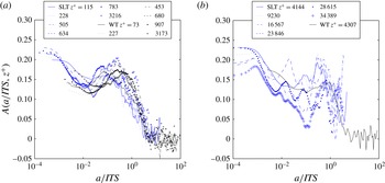
. The asymmetry index is plotted in figure 6(a) for different scales, at different heights, for both WT and SLT datasets. As outlined in the introduction, a hump is observed in a range of scales smaller than the
 $ITS$
in both datasets, consistent in terms of frequency and amplitude with the hump reported by Basu et al. (Reference Basu, Foufoula-Georgiou, Lashermes and Arnéodo2007). Here we confirm the location of the hump in the inertial range using an independent dataset from atmospheric surface layer (SLT) and a new wind tunnel experiment (WT).
Asymmetry index of the streamwise velocity increments as a function of scale for WT (black lines) and SLT (blue lines) at
 $70<z^{+}<3.3\times 10^{3}$
(a) and at
 $z^{+}>4\times 10^{4}$
(b). The
 $x$
-axis represents the time scale
 $a$
normalized by the
 $ITS$
.

3.3 Reynolds-number-independent asymmetry in turbulent boundary layers
As the difference in Reynolds number between SLTEST and the SAFL wind tunnel is of the order of two decades, the emerging hump-like feature might be universal to turbulent boundary layer flows. One of the main objectives of this paper is to compare systematically the amplitude and location of the hump at varying wall-normal distances, providing different normalization options for both the vertical coordinate
 $z$
and the velocity increment time scale
 $a$
. The main hypothesis put forward is how the asymmetry index evolves in different regions of the turbulent boundary layer, for the two available Reynolds-number experiments. In order to allow a direct comparison between the laboratory-scale (WT) and field-scale (SLT) datasets, we kept a consistent normalization for
 $a$
, using the integral time scale for normalization,
 $a/ITS$
.
As discussed earlier in the introduction, scale interactions near the wall are the main source of intermittency and anisotropy observed in high-order statistics of the streamwise velocity (Guala et al.
Reference Guala, Metzger and McKeon2010, Reference Guala, Metzger and McKeon2011; Singh et al.
Reference Singh, Howard and Guala2014). In the continuous cycle of mutual influence between (inner) near-wall turbulence and (outer)
 ${\it\delta}$
-scale motions, we argue that a single scaling may not work across the whole range of turbulent scales and wall distances. For this purpose, we investigate here if inner (
 $z^{+}=zu_{{\it\tau}}/{\it\nu}$
) or outer (
 $z/{\it\delta}$
) unit normalization will lead to a collapse of the anisotropy (asymmetry index) curves
 $A(a,z)$
for a specific range of temporal scales
 $a$
and vertical locations
 $z$
. In this respect, we recall that the spacing between near-wall streaks (
 $\simeq 100$
viscous wall units) has been proved to be fairly invariant across a wide range of Reynolds number (Metzger & Klewicki Reference Metzger and Klewicki2001). Recognizing the key role of near-wall structures to inner–outer scale interaction processes, we first attempt to use the viscous scale
 ${\it\nu}/u_{\ast }$
for wall distance normalization. We compare scale-dependent asymmetry curves for the two datasets at the fixed
 $z^{+}$
location in figure 6(a,b). Here the normalizing time scale for the velocity increment is kept as
 $ITS$
, which of course varies in the two Reynolds-number flows.
In figure 6(a), we note how the hump maintains its amplitude and temporal location for a wide range of
 $z^{+}$
, independent of the Reynolds number, unambiguously marking a statistical property of turbulent boundary layer flows. However, for
 $z^{+}>4000$
(figure 6
b), we start to notice appreciable deviations for large time scales
 $a$
approaching the
 $ITS$
, suggesting a change in scale interaction processes, and possibly in wall turbulence organization at the SLT high-Reynolds-number flow. For even larger wall distances, inspected in figure 6(b), the asymmetry peak is lost within ample oscillations that might be the result of the interactions between large- and very-large-scale motions populating the logarithmic layer of the SLT flow; in such a case, we must note that the SLT dataset may not be long enough to ensure statistical convergence of the scale-dependent asymmetry index in the full temporal–vertical domain investigated. This said, figure 6(b) confirms that the flow region where asymmetry statistics overlap is confined in the
 $O(10^{2}{-}10^{3})$
range of viscous wall units. Note that an independent set of data from a wind tunnel experiment (not shown here) showed similar trends and results to those presented here.
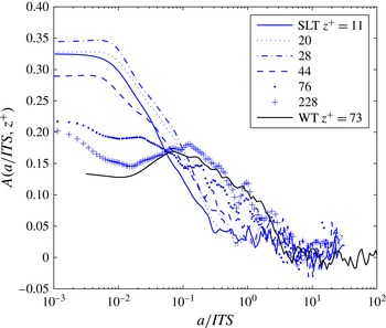
Asymmetry index of the streamwise velocity increments as a function of scale for WT (black line) and SLT (blue lines) for
 $z^{+}<10^{2}$
. The
 $x$
-axis represents the time scale
 $a$
normalized by the
 $ITS$
.

The SLT data provide the opportunity to further explore the scale-dependent asymmetry very close to the wall (
 $z^{+}<100$
; see figure 7). As the surface is approached, the amplification of
 $A(a,z)$
in the Kolmogorov scale range contributes to increase the peak value while smearing the hump signature. With intermittency and small-scale asymmetry both high at the wall, scale coupling is inferred to occur within a different layer and population of wall turbulent structures, as compared to the case discussed above in the logarithmic layer. Following a structural interpretation, figure 7 suggests a strong effect of large- and very-large-scale motions at the surface, where the mean shear is strongest, literally sweeping the wall and distorting the distribution of the near-wall streamwise velocity at those small scales that were traditionally marked as homogeneous and isotropic. Recently Hultmark et al. (Reference Hultmark, Vallikivi, Bailey and Smits2013) quantified third-order central moments of velocity fluctuations obtained at high Reynolds number and observed increasing skewness with decreasing wall-normal distance. These observations are in qualitative agreement with our results, suggesting that scale coupling increases as the wall distance decreases. The evolution of the asymmetry peak appears to occur quite sharply in the
 $(a,z)$
domain, suggesting a marked change in the wall structure organization. This is consistent with the spatial transition between the near-wall streaks and the ramp-like structure organization above
 $z^{+}\sim 70$
, which marks the lower end of the logarithmic layer. With increasing distance from the wall (
 $10<z^{+}<50$
), the streaks’ asymmetry is reduced at the small time scales, until the hump
 $z^{+}>70$
clearly emerges in the temporal (inertial range) and wall-normal domain of the attached eddies (see Perry, Henbest & Chong Reference Perry, Henbest and Chong1986).
The
 $A(a,z)$
vertical distribution suggests that local high shear induced by large-scale structures impinging the wall is felt by near-wall streaks, leading to increased intermittency (see Guala et al.
Reference Guala, Metzger and McKeon2010, and also figure 4
b), asymmetry and non-local energy transfer (Warhaft Reference Warhaft2002; Singh et al.
Reference Singh, Howard and Guala2014). The asymmetry profiles also indicate that the ramp-like structures inferred in Guala et al. (Reference Guala, Metzger and McKeon2011) to populate, at the atmospheric scale (high Reynolds number), a relatively near-wall region of the boundary layer up to
 $z^{+}\sim 5\times 10^{3}$
display the asymmetry-hump signature in the same vertical range. The role of ramp-like structures is confirmed by employing the attached eddy time scale
 $z/u_{\ast }$
as a replacement for the
 $ITS$
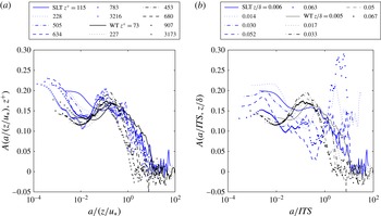
: in figure 8(a), asymmetry curves in the near-wall region are presented as a function of
 $a/(z/u_{\ast })$
and observed to partially overlap across a range of scales consistent with those reported in figure 6(a).
(a) Asymmetry index of the streamwise velocity increments as a function of scale for WT (black lines) and SLT (blue lines) at
 $z^{+}<10^{3}$
. (b) Asymmetry index of the streamwise velocity increments as a function of scale for WT (black lines) and SLT (blue lines) for comparable
 $z/{\it\delta}$
locations. The
 $x$
-axis in (a) represents the time scale
 $a$
normalized by
 $z/u_{\ast }$
, whereas in (b) it represents the time scale
 $a$
normalized by the
 $ITS$
.

The validity of inner, viscous, scaling and its conceptual implications are further evidenced in figure 8(b). When asymmetry index curves are compared for both WT and SLT at different
 $z^{+}$
but similar
 $z/{\it\delta}$
locations, no significant data collapse is observed. Near-wall scaling is thus confirmed in a region well above the near-wall spectral peak of Hutchins & Marusic (Reference Hutchins and Marusic2007a
) and well within the logarithmic layer, where outer scaling would have been, in principle, an equally valid option. While we acknowledge that a full comparison should be carried out using measurements in the outer layer at the SLTEST Reynolds number (not available here), we must recognize that strong scale interactions, intermittency and anisotropy are typically observed in high-shear flows, thus naturally residing in the near-wall region. Therefore, it is speculated that outer scale normalization for
 $A(a,z)$
will hardly apply in large-scale geophysical flows, and that the asymmetry hump will remain a near-wall turbulence signature, with near wall defined in viscous units.
4 Summary and conclusions
The distribution of scale-dependent streamwise velocity increment
 ${\rm\Delta}u(a,z)=u(t+a,z)-u(t,z)$
was investigated at varying wall-normal locations in turbulent boundary layer flows at laboratory and atmospheric Reynolds numbers, using measurements from the SAFL wind tunnel and the SLTEST site (Metzger et al.
Reference Metzger, McKeon and Holmes2007). The fifth-order moment of the velocity increments was employed here to emphasize the scale-dependent non-Gaussianity of the increment distribution, leading to the definition of the scale-dependent asymmetry index
 $$\begin{eqnarray}A(a,z)=\frac{\langle ({\rm\Delta}u(a,z)-\overline{{\rm\Delta}u(a,z)})^{3}\rangle }{\langle |({\rm\Delta}u(a,z)-\overline{{\rm\Delta}u(a,z)})^{3}|\rangle }.\end{eqnarray}$$
The shape of
 $A(a,z)$
revealed a well-defined hump located in the inertial range, thus for time scales
 $a$
smaller than the
 $ITS$
and larger than the Kolmogorov scale
 ${\it\tau}_{k}$
. The hump is observed for
 $z^{+}<5\times 10^{3}$
, with peak location at time scale
 $a/ITS\sim a/(z/u_{\ast })\sim 0.1$
, and amplitude
 $A(a,z)\sim 0.2$
, with a tendency to shift towards smaller time scales as the surface is approached (
 $z^{+}<10^{2}$
). The asymmetry hump location in the temporal and vertical domain is observed to obey inner wall scaling, while outer-scale normalization, i.e. comparing
 $A(a,z)$
curves at similar
 $z/{\it\delta}$
, did not seem to provide any useful insight. By comparing the two datasets, the hump in
 $A(a,z)$
emerged as a robust, statistical feature of the canonical turbulent boundary flow, independent of the Reynolds number.
A parallel analysis using magnitude cumulant analysis of the scale-dependent velocity increments revealed that intermittency is also enhanced near the wall, well within the logarithmic region, in the same domain where the hump signature was observed. The combination of asymmetry and intermittency is inferred to point at non-local energy transfer, i.e. between non-neighbouring scales in the frequency domain. From a turbulent structure perspective this is an indication of strong scale interaction processes (Warhaft Reference Warhaft2002; Guala et al.
Reference Guala, Metzger and McKeon2011): outer-scale motions in the logarithmic layer are inferred to impact and distort small scales near the wall, favouring abrupt energy transfer across scales, bypassing the typically assumed energy cascade of the inertial range, and causing rare but highly dissipative events that leave a mark on high-order statistics. The asymmetry peak at small scales for
 $z^{+}<70$
suggests that near-wall streaks are mostly affected; in addition, evidence of the asymmetry hump up to
 $z^{+}\sim 5000$
implies that also ramp-like structures are likely to be modulated, denoting a wide range of multi-scale interactions in a significant portion of the wall region. The fact that the attached-eddy scaling
 $z/u_{\ast }$
and inner normalization (
 $z^{+}$
) lead to a collapse of the
 $A(a,z)$
curves further suggests that ramp-like structures probably obey near-wall scaling as opposed to outer scaling, as inferred in Guala et al. (Reference Guala, Metzger and McKeon2011).
We acknowledge that the observed oscillations of the asymmetry index for large time scales, estimated from the atmospheric (SLT) dataset, may be due to the finite length of the velocity time series that may affect the convergence of high-order statistics at large scales. In addition, the increased intermittency observed near the wall in the SLT data, and (to some extent) far from the wall in the WT data, points at a broader question on the effect of the intensity and vertical distribution of the mean shear on the structure of turbulence. Intermittency has been observed to be enhanced in shear flows as compared to homogeneous isotropic turbulence, exhibiting some (Antonia et al.
Reference Antonia, Orlandi and Romano1998; Onorato et al.
Reference Onorato, Camussi and Iuso2000) or minimal (Toschi et al.
Reference Toschi, Leveque and Ruiz-Chavarria2000) wall-normal dependence. Ruiz-Chavarria et al. (Reference Ruiz-Chavarria, Ciliberto, Baudet and Lévêqueb2000) evidenced that different scaling regions in the structure functions can affect the estimates of height-dependent and scale-dependent intermittency. Additionally, measurements in the atmospheric boundary layer at
 $O(10^{2})$
m over urban or coastline areas revealed strong intermittency at large (time) scales (Boettcher et al.
Reference Boettcher, Renner, Waldl and Peinke2003; Liu et al.
Reference Liu, Hu, Cheng and Song2010).
For all these reasons, it would be important to confirm (or discuss) the trends outlined in this paper using other datasets from canonical boundary layer flows at high Reynolds number.
Acknowledgements
We thank Professors M. Metzger and B. J. McKeon for providing the SLTEST data. We also thank the editor, I. Marusic, and the three reviewers, whose suggestions and constructive comments substantially improved our presentation and refined our interpretations. This research has been supported by our own curiosity and partially by National Science Foundation (NSF) Career Grant Geophysical Flow Control to M.G.