


1. Introduction
Concerns about climate change mitigation are leading to growing interest in renewable energy and, together with declining costs of solar, are driving a rapid increase in solar energy deployment in the United States (US). Solar photovoltaic (PV) is projected to supply between 20% and 42% of US electricity generation by 2050 (Gagnon et al., Reference Gagnon, Brown, Cole, Pham, Hamilton, Awara, Barlas, Brown, Carag, Cohen and Chen2024). Utility-scale solar is the fastest-growing segment of solar energy deployment and is land-intensive, requiring 3–10 acres per megawatt direct current (MWdc)Footnote 1 of installed capacity (Bolinger & Bolinger, Reference Bolinger and Bolinger2022; Ong et al., Reference Ong, Campbell, Denholm, Margolis and Heath2013). Anticipated growth in solar energy deployment is expected to require 4–11 million acres of land by 2050 (US Department of Energy, 2021).
Agricultural croplands coincide with areas favorable to solar energy deployment (Macknick et al., Reference Macknick, Hartmann, Barron-Gafford, Beatty, Burton, Choi, Davis, Davis, Figueroa, Garrett, Hain, Herbert, Janski, Kinzer, Knapp, Lehan, Losey, Marley, MacDonald, McCall, Nebert, Ravi, Schmidt, Staie and Walston2022), and they often have the highest productivity for PV energy generation (Adeh et al., Reference Adeh, Good, Calaf and Higgins2019). The available solar insolation, stable soil conditions, and inherently flat agricultural lands reduce project risks for solar developers (Macknick et al., Reference Macknick, Hartmann, Barron-Gafford, Beatty, Burton, Choi, Davis, Davis, Figueroa, Garrett, Hain, Herbert, Janski, Kinzer, Knapp, Lehan, Losey, Marley, MacDonald, McCall, Nebert, Ravi, Schmidt, Staie and Walston2022). Other characteristics of farms favorable for solar energy are nearby interconnection access to the electric grid, to roads, and to water for panel cleaning if needed (Macknick et al., Reference Macknick, Hartmann, Barron-Gafford, Beatty, Burton, Choi, Davis, Davis, Figueroa, Garrett, Hain, Herbert, Janski, Kinzer, Knapp, Lehan, Losey, Marley, MacDonald, McCall, Nebert, Ravi, Schmidt, Staie and Walston2022). Declining costs of PV technology and rising market and policy incentives for solar energy have led PV developers to offer land lease rates that are three to four times higher than the returns to row crop production (Bookwalter, Reference Bookwalter2019; Sorensen et al., Reference Sorensen, Nogeire and Hunter2022). This, together with the risks of crop farming, is leading to increasing conversion of cropland to solar farming (Walston et al., Reference Walston, Li, Hartmann, Macknick, Hanson, Nootenboom, Lonsdorf and Hellmann2021). Illinois is one of the fastest-growing states for solar deployment (Maguire et al., Reference Maguire, Tanner, Winikoff and Williams2024; Sorensen et al., Reference Sorensen, Nogeire and Hunter2022).Footnote 2
This has led to concerns about solar farms displacing food/feed crop production and community opposition to solar development, similar to those with wind energy, biofuels and oil and gas developments (Moore et al., Reference Moore, Graff, Ouellet, Leslie, Olweean and Wycoff2021; Petrova, Reference Petrova2013; Susskind et al., Reference Susskind, Chun, Gant, Hodgkins, Cohen and Lohmar2022).Footnote 3 Many jurisdictions now prohibit large-scale solar farms on agricultural land (SEIA, 2021; Sorensen et al., Reference Sorensen, Nogeire and Hunter2022). Solar developers also cite community opposition as one of the leading causes of project delays and cancellations (Rand et al., Reference Rand, Hoesch, Mills, Hoen, Nilson, Bessette and White2024; Susskind et al., Reference Susskind, Chun, Gant, Hodgkins, Cohen and Lohmar2022).
Interest in maintaining crop production while also enabling solar farming is leading to growing attention on Agrivoltaic (AV) technology, defined here as the dual use of land with crops and panel rows interspersed with each other (Barron-Gafford et al., Reference Barron-Gafford, Pavao-Zuckerman, Minor, Sutter, Barnett-Moreno, Blackett, Thompson, Dimond, Gerlak, Nabhan and Macknick2019; Cuppari et al., Reference Cuppari, Fernandez-Bou, Characklis, Ramirez, Nocco and Abou-Najm2024; Dupraz et al., Reference Dupraz, Marrou, Talbot, Dufour, Nogier and Ferard2011; Moore et al., Reference Moore, Graff, Ouellet, Leslie and Olweean2022). AV installations can take various forms, from planting pollinator-friendly crops, specialty and other crops, and pasture grasses to animal grazing sites; there is a growing literature analyzing the biophysical and ecological implications of AV systems and their profitability (Barron-Gafford et al., Reference Barron-Gafford, Pavao-Zuckerman, Minor, Sutter, Barnett-Moreno, Blackett, Thompson, Dimond, Gerlak, Nabhan and Macknick2019; Hernandez et al., Reference Hernandez, Hoffacker, Murphy-Mariscal, Wu and Allen2015; Gomez-Casanovas et al., Reference Gomez-Casanovas, Mwebaze, Khanna, Branham, Time, DeLucia, Bernacchi, Knapp, Hoque, Du, Blanc-Betes, Barron-Gafford, Peng, Guan, Macknick, Miao and Miljkovic2023). However, there has been no comprehensive assessment of the costs and benefits of AV with row crop systems in the US Midwest context from both the developer’s and farmer’s perspective.
This study aims to address several research objectives related to the economic and biophysical effects of AV systems in the Midwestern context, with corn and soybeans as the dominant crops. First, we develop a conceptual framework to analyze the determinants of the profitability of an AV system relative to PV-only for a solar developer and relative to Crop-only or PV-only for a farmer. We analyze the conditions under which both a solar developer and the landowner would have an economic incentive to adopt an AV system instead of PV-only or Crop-only. We also compare the profitability of an AV system with that of a field on which PV and crops are produced adjacent to each other (and referred to as Adjacent Agriculture-PV (AAPV)) (see definitions in Table 1). The latter configuration reflects a common scenario in which a farmer allocates only a portion of their land, potentially marginal or less productive areas, to solar development while maintaining crop production on the remainder. The AAPV is not an AV system; we include it here for comparison as an alternative configuration for producing solar energy and food crops on the same field.
Description of alternative configurations of solar panels and crops

Table 1. Long description
The diagram displays six distinct land-use scenarios for solar energy and agriculture.
* Top-left panel: Integrated A V (I A V). Shows ground-mounted P V panels elevated at 8 feet with 43.5 feet of spacing between rows. A tractor is shown farming the land between the panel rows.
* Top-center panel: Tall Panels A V (T A V). Features panels elevated to 12 feet with 18 feet of spacing. This height allows farming directly underneath the panels, covering 93 percent of the crop area.
* Top-right panel: Adjacent Agriculture-P V (A A P V). Shows a split field where P V panels at 4 feet height are clustered on one side and crops are grown on the other side, with no spatial integration.
* Bottom-left panel: Reduced Buffer A V (R A V). Similar to I A V with 8-foot high panels and 43.5-foot spacing, but uses autonomous equipment to farm closer to the panel supports, increasing crop area to 76 percent.
* Bottom-center panel: P V-only. Shows a standard utility-scale solar farm with 4-foot high panels and 18-foot spacing. The entire 80-acre area is dedicated to P V with 0 percent crop area.
* Bottom-right panel: Crop-only. Shows a traditional open field with 100 percent crop area and no P V panels.
Notes:
-
1. Figures in brackets are percentages of the crop and PV area.
-
2. In the IAV configuration, the farming width between PV rows is 30 ft, and the buffer is 3 ft for 28 PV rows.
-
3. In the TAV design, the farming width is 18 ft, while the farming buffer is reduced to −4 ft, giving 70 PV rows.
-
4. Similar to PV-only, the AAPV configuration has a spacing of 18 ft and 28 PV rows in total.
-
5. In the RAV configuration, the farming width is increased to 40 ft, while the buffer is reduced to −2 ft compared to the IAV configuration.
We define and analyze the determinants of the breakeven price of electricity and the breakeven cost of electricity generation with AV. These are defined as the price (or cost of electricity) at which AV generates the same level of profit as a competing land-use configuration (e.g. PV-only or AAPV). This reflects the decision problem typically faced by solar developers, who aim to maximize returns by selecting the most profitable configuration for a given site. We also analyze the breakeven price of crop output that would make the profits for a farmer from an AV system equal to those with alternative land uses (PV-only, Crop-only or AAPV). If the AV offers lower profits than PV-only, developers are unlikely to adopt it unless electricity prices rise, capital costs fall, or other non-monetary incentives (e.g. community acceptance or policy mandates) influence their choice. Thus, breakeven comparisons in this study serve as thresholds for equal profitability across land-use options, rather than merely assessing project viability.
Second, we combine an Agricultural Production Systems Simulator (APSIM) Soybean Model and a Solar Analysis Model with a benefit–cost analysis to quantify the effects on crop and energy yield and profitability of three different AV systems and that of AAPV compared to PV-only or Crop-only production systems for a representative field managed using conventional technology in the US Midwest. The three alternative configurations of an AV system analyzed are (a) interspersed rows of crop and panels with buffer areas between the two (referred to as Integrated AV (IAV)); (b) the same as (a) but with reduced buffer areas (RAV); and (c) tall panels with crops grown underneath them (Tall Panels AV (TAV)) (see Table 1). Growing crops interspersed with solar panels will require raising panel height and also increasing space between panels to allow conventional farm equipment to conduct field operations between panels (Horowitz et al., Reference Horowitz, Ramasamy, Macknick and Margolis2020; Shindele et al., Reference Shindele, Trommsdorff, Schlaak, Obergfell, Bopp, Reise, Braun, Weselek, Bauerle, Högy, Goetzberger and Weber2020). Corn and soybeans are the dominant crops in the US Midwest. Given the high costs of raising panel height, we focus on analyzing the profitability of AV with soybeans since growing corn in an AV system would necessitate even higher panels. Production of crops interspersed with solar panels or underneath panels can affect crop yields because of the limited availability of solar radiation. In contrast, an AAPV system with a portion of the field dedicated to PV and the remaining portion dedicated to crops does not require modifications to panel height or spacing and does not cause adverse impacts of shading on crops.
We apply the APSIM model to analyze the implications of AV systems for land productivity compared to PV-only and Crop-only systems. An AV system can create competition between solar radiation available for solar energy generation and crop production, depending on the density and height of panels. Shading of crops by the panels can have positive or negative effects on crop yield depending on the shade tolerance of the crop and climatic conditions (Barron-Gafford et al., Reference Barron-Gafford, Pavao-Zuckerman, Minor, Sutter, Barnett-Moreno, Blackett, Thompson, Dimond, Gerlak, Nabhan and Macknick2019; Weselek et al., Reference Weselek, Ehmann, Zikeli, Lewandowski, Shindele and Högy2019, Reference Weselek, Bauerle, Hartung, Zikeli, Lewandowski and Högy2021). They can also positively or negatively affect the solar energy yield relative to PV alone (Barron-Gafford et al., Reference Barron-Gafford, Pavao-Zuckerman, Minor, Sutter, Barnett-Moreno, Blackett, Thompson, Dimond, Gerlak, Nabhan and Macknick2019; Williams et al., Reference Williams, Hashad, Wang and Max Zhang2023). Additionally, while AV can allow dual use of land, it can also lead to some land that cannot be used for either energy or crop production because a buffer area is required between panels and crops to allow operation of equipment without damaging the panels. As a result, total crop production may decline more than proportionately to the reduction in the cropped area in an AV field relative to Crop-only.
We compare the effects of the three AV configurations with those of AAPV, PV-only and Crop-only on the combined crop and solar energy productivity, as measured by the Land Equivalent Ratio (LER) (Dupraz et al., Reference Dupraz, Marrou, Talbot, Dufour, Nogier and Ferard2011; Gomez-Casanovas et al., Reference Gomez-Casanovas, Mwebaze, Khanna, Branham, Time, DeLucia, Bernacchi, Knapp, Hoque, Du, Blanc-Betes, Barron-Gafford, Peng, Guan, Macknick, Miao and Miljkovic2023; Mamun et al., Reference Mamun, Dargusch, Wadley, Zulkarnain and Aziz2022; Weselek et al., Reference Weselek, Ehmann, Zikeli, Lewandowski, Shindele and Högy2019). The LER is defined as the sum of the ratio of crop yield under the AV system to Crop-only and the ratio of PV energy under the AV to PV-only system (Dupraz et al., Reference Dupraz, Marrou, Talbot, Dufour, Nogier and Ferard2011; Schweiger & Pataczek, Reference Schweiger and Pataczek2023; Trommsdorff et al., Reference Trommsdorff, Vorast, Durga and Padwardhan2021). An LER greater than 1 implies that the combined productivity with the dual land use under the AV systems is higher than productivity under a single land use. A high LER may not be sufficient to drive the adoption of AV unless it is also accompanied by higher profitability of AV in comparison to PV-only or Crop-only production. LER measures relative productivity in physical units and does not consider differences in energy and crop prices, revenues and costs, which affect profitability. Economic factors, such as the relative price of crops and electricity, may lower the profitability of AV despite an LER greater than one.
Lastly, we analyze the relationship between the LER and the profitability of an AV system by integrating the simulated effects of alternative AV systems on energy and crop yield relative to PV-only and Crop-only systems with estimates of the costs and revenues of these alternative systems. We consider the timing of benefits and costs over the assumed 25-year lifetime of a PV system and determine the net present value of their profitability using a discount rate. We assess the annualized profit of each of these systems and analyze the relationship between LER and the profitability of an AV system relative to PV-only or Crop-only systems.
There is a growing literature analyzing the effects of AV systems on crop yields. Studies show that the impacts of AV on crop yields depend on many variables, including the shade-tolerance of the crop, the design configuration of the PV panels and their distance apart (Barron-Gafford et al., Reference Barron-Gafford, Pavao-Zuckerman, Minor, Sutter, Barnett-Moreno, Blackett, Thompson, Dimond, Gerlak, Nabhan and Macknick2019; Campana et al., Reference Campana, Stridh, Amaducci and Colauzzi2021; Weselek et al., Reference Weselek, Ehmann, Zikeli, Lewandowski, Shindele and Högy2019). The effect of shading varies with the shade tolerance of the crop; a meta-analysis showed that berries, fruits and fruity vegetables benefited from a reduction in solar radiation, while forages and leafy vegetables experienced small reductions in yield. In contrast, maize and grain legumes experienced larger crop yield losses even at low shade levels (Laub et al., Reference Laub, Pataczek, Feuerbacher, Zikeli and Högy2022). A few studies have analyzed the effect on corn yields of growing it underneath tall panels with varying densities of panels in Japan (Sekiyama & Nagashima, Reference Sekiyama and Nagashima2019) and the US Midwest (Gupta et al., Reference Gupta, Gruss, Cammarano, Brouder, Bermel, Tuinstra, Gitau and Agrawal2024; Turnley et al., Reference Turnley, Grant, Schull, Cammarano, Sesmero and Agrawal2024). These studies find that low-density shading has negligibly negative or even positive effects on yield, while high panel density leads to large negative effects on yield. In contrast, our study evaluates various AV configurations with soybeans, assessing their impact on crop yield, energy generation, land use efficiency and profitability, providing a more detailed analysis of the trade-offs and synergies between crop production and energy generation in the US Midwest.
Several studies have examined the LER of AV systems (Amaducci et al., Reference Amaducci, Yin and Colauzzi2018; Campana et al., Reference Campana, Stridh, Amaducci and Colauzzi2021; Dupraz et al., Reference Dupraz, Marrou, Talbot, Dufour, Nogier and Ferard2011; Schweiger & Pataczek, Reference Schweiger and Pataczek2023; Toledo & Scognamiglio, Reference Toledo and Scognamiglio2021; Trommsdorff et al., Reference Trommsdorff, Vorast, Durga and Padwardhan2021) and found that AV systems with mostly shade-tolerant crops result in LER values greater than 1. Few studies have examined the relationship between LER and AV profitability. There are also only a few studies on the profitability of AV systems compared to crops or solar-only options, and most of these have focused on specialty crops (Dinesh & Pearce, Reference Dinesh and Pearce2016; Mamun et al., Reference Mamun, Dargusch, Wadley, Zulkarnain and Aziz2022; Thompson et al., Reference Thompson, Bombelli, Shubham, Watson, Everard, D’Ardes, Schievano, Bocchi, Zand, Howe and Bombelli2020). Several studies find higher profits for AV with speciality crops, such as lettuce, basil, spinach and other vegetables, than crops alone (Dinesh & Pearce, Reference Dinesh and Pearce2016; Thompson et al., Reference Thompson, Bombelli, Shubham, Watson, Everard, D’Ardes, Schievano, Bocchi, Zand, Howe and Bombelli2020). These higher profits result from the additional energy revenues compared to a crop-only system and increased yields of shade-tolerant crops (Mamun et al., Reference Mamun, Dargusch, Wadley, Zulkarnain and Aziz2022). However, these studies have not compared the profitability of AV systems relative to PV alone and whether solar developers would be incentivized to invest in the AV system. In the case of row crops, studies with cereal farming systems in Germany (Feuerbacher et al., Reference Feuerbacher, Laub, Högy, Lippert, Pataczek, Shindele, Wieck and Zikeli2021, Reference Feuerbacher, Herrmann, Neuenfeldt, Laub and Gocht2022) and rice farming across six countries (Vietnam, Bangladesh, China, Egypt, Brazil and India) (Sojib Ahmed et al., Reference Sojib Ahmed, Rezwan Khan, Haque and Ryyan Khan2022) found that crop yields decline substantially in an AV system relative to crops alone and that electricity prices for an AV system would need to be significantly higher than under PV alone to make AV profitable. These studies have compared the profitability of AV systems relative to crops alone but not to PV alone. Furthermore, while they show increased profits of AV compared to crops for several locations, it is unclear if their findings would apply to row crops in the US Midwest.
Our analysis of AV systems with soybeans in the US Midwest shows that while some AV configurations can improve land-use efficiency (LER > 1), they will require additional land to achieve equivalent crop output as a Crop-only system and will not be as profitable as PV-only for the solar developer or the farmer without policy support. These findings underscore the tradeoffs with AV systems with row crops and the necessity of considering implications for both crop and solar energy producers in analyzing incentives for their adoption. The rest of the paper is organized as follows. The next section describes the conceptual framework for analyzing the economic drivers to adopt an AV system and its relationship to LER. This is followed by a description of the models used to determine the effects of an AV system on crop yield and solar energy under various configurations of AV systems and the data used for the study. We then describe the results and conclude with a discussion of their implications for scaling AV systems in the US Midwest.
2. Conceptual framework
We now present a benefit–cost analysis framework to compare the profitability of the IAV system with PV-only and Crop-only for a representative field. We first present the framework to compare the net present value of returns per unit of land with IAV relative to those with a PV-only per unit of land from a solar developer’s perspective. We assume that for an IAV system to be adopted by a solar developer, it must be more profitable than PV-only per unit of land. Next, we present the framework for analyzing the decision of a landowner to choose an IAV system by comparing its net present value per unit of land relative to that of producing a Crop only or leasing the entire land for PV. Following that, we present the framework to compare the profitability differences between integrated and adjacent land-use strategies for solar energy and crop production by analyzing the combined profits from an IAV field to those from a field in which solar panels and crops are spatially separated, referred to as AAPV.
The framework below considers the profitability of a specific space and panel height configurations for IAV, which exogenously determine the share of land x under PV and the rest (1-x) under crop production. This enables us to examine the conditions under which an IAV configuration could be profitable relative to PV alone for a developer or relative to crop production alone for a farmer and its implications for policy incentives needed.
2.1. The solar developer’s choice problem
We represent the annualized profits per acre,
$ {\pi}_S^{PV} $
 , for a solar developer from a PV-only system by

where
$ {S}^{PV} $
 is the annual solar energy output from the PV-only system (MWh/year/acre);
$ {P}_S^{PV} $
 is the price of solar electricity under a PV-only system ($/MWh);Footnote 4
$ {LCOE}^{PV} $
 is the levelized cost of solar energy under PV-only ($/MWh) and is defined in more detail in Section 3.2; M is the annual vegetation management cost ($/acre), and L is the annual cost of leasing the land ($/acre).Footnote 5 Profits and costs of solar energy vary over the life time of the installation, resulting in a time-varying stream of costs and revenues over the 25-year project life. For ease of algebraic representation, all profit and cost expressions in this framework are annualized values derived from the net present value of costs and revenues over the 25-year project life, using a constant discount rate.
Suppose that the developer is considering adopting an IAV system in which a share x of the 1-acre field will be under PV and (1−x) will be under crop production. In this setup, the solar developer pays the landowner both an annual lease payment for the use of the land under PV and a vegetation management fee to maintain ground cover around the solar panels – a practice commonly reported in focus group discussions with farmers. These arrangements shift vegetation maintenance responsibilities to the farmer while compensating them for this service. The returns per acre for the solar developer on the portion of land that is under PV in an IAV system are thus represented by

where
$ {\pi}_S^{IAV}/x $
 is the annual profit per acre from the land under PV in the IAV system for the solar developer;
$ {S}^{IAV} $
 is the annual solar energy output from the IAV portion of the field (MWh/year),
$ {P}_S^{IAV} $
 is the price of electricity under the IAV system ($/MWh) (that may or may not be the same as
$ {P}_S^{PV} $
 and
$ {LCOE}^{IAV} $
 is the levelized cost of solar energy generation under the IAV system ($/MWh). We expect
$ {LCOE}^{IAV} $
 ≥
$ {LCOE}^{PV} $
 . We denote
$ {S}^{IAV}=x{\delta}_S{S}^{PV} $
 where
$ {\delta}_S\gtreqless $
 1. Thus:
$ {\pi}_S^{IAV}=x{\delta}_S{S}^{PV}\left({P}_S^{IAV}-{LCOE}^{IAV}\right)-x\left(L+M\right) $
 . Specifically, we define
$ {\delta}_S $
 as the energy output per unit of land area under solar panels in an IAV system relative to PV-only, which depends on IAV design and environmental factors. Recent studies suggest that IAV systems can achieve similar or modestly higher energy yields compared to PV-only systems, largely due to elevated panel heights and cooling effects from underlying vegetation, which can lower panel temperatures (Barron-Gafford et al., Reference Barron-Gafford, Pavao-Zuckerman, Minor, Sutter, Barnett-Moreno, Blackett, Thompson, Dimond, Gerlak, Nabhan and Macknick2019; Miljkovic et al., Reference Miljkovic, Du, Solecki, Hoque, Garimella, Jia, Peng, Mwebaze, McCall, Majeed, Time, Kim, Sturchio, Guan, Khanna, Bernacchi, Lee, Knapp, Barron-Gafford and Branham2024; Williams et al., Reference Williams, Hashad, Wang and Max Zhang2023). However, these gains are not uniform and can vary depending on site-specific factors such as climate, crop type and system design – some studies even report slight reductions in yield under certain conditions (Macknick et al., Reference Macknick, Hartmann, Barron-Gafford, Beatty, Burton, Choi, Davis, Davis, Figueroa, Garrett, Hain, Herbert, Janski, Kinzer, Knapp, Lehan, Losey, Marley, MacDonald, McCall, Nebert, Ravi, Schmidt, Staie and Walston2022).
We assume that the solar developer will have an economic incentive to adopt IAV if the profit per unit of land from the share of land under PV in the IAV system is larger than or equal to the profit per unit of land from a stand-alone PV system. That is, the solar developer will choose the IAV system if
$ {\pi}_S^{IAV}/x\ge {\pi}_S^{PV} $
 , which implies that IAV will be chosen if:

Note that the term (L + M) – representing lease and vegetation management payments to the farmer – cancels out on both sides of the inequality. This leads to a simplified profitability condition that can be solved to determine the breakeven price of electricity,
$ {P}_S^{\ast IAV} $
 at which an IAV system becomes as profitable as a PV-only system for the solar developer:


Since
$ {LCOE}^{IAV} $
 is greater than
$ {LCOE}^{PV} $
 , it implies that the breakeven price
$ {P}_S^{\ast IAV} $
 is greater than
$ {P}_S^{PV} $
 if
$ {\delta}_S $
 is equal to 1. Additionally,
$ {P}_S^{\ast IAV} $
 increases as
$ {LCOE}^{IAV} $
 increases and as
$ {\delta}_S $
 decreases, since we expect that
$ {P}_S^{PV}-{LCOE}^{PV}\ge 0 $
 . On the other hand, as
$ {\delta}_S $
 increases above 1 and the IAV system produces more electricity than the PV-only system – perhaps due to cooler microclimates from crops, or other synergies, then the required breakeven price for electricity under IAV (
$ {P}_S^{\ast IAV} $
 ) decreases. The difference between the breakeven price of electricity under IAV and the prevailing electricity price under PV-only (
$ {P}_S^{\ast IAV}-{P}_S^{PV} $
 ) represents the feed-in tariff or price premium required to make IAV systems economically competitive.
Alternatively, if the price of electricity is the same under the IAV system and the PV-only system (
$ {P}_S^{IAV}={P}_S^{PV} $
 ), then we can solve for the breakeven value of the levelized cost of electricity (LCOE) in the IAV system (
$ {LCOE}^{\ast IAV} $
 ) as follows:

If
$ {\delta}_S $
 =1, then the breakeven
$ {LCOE}^{\ast IAV} $
 must be equal to
$ {LCOE}^{PV}. $
 If solar developers are just breaking even with PV-only, then (6) indicates that
$ {LCOE}^{\ast IAV} $
 must be equal to
$ {P}_S^{PV} $
 . For other cases,
$ {LCOE}^{\ast IAV} $
 could be higher or lower than
$ {LCOE}^{PV} $
 . The difference between the breakeven LCOE for IAV and the actual or prevailing LCOE of IAV (
$ {LCOE}^{\ast IAV}-{LCOE}^{IAV} $
 ) represents the production tax credit required to make IAV economically viable relative to PV-only. By expressing the breakeven conditions in terms of both electricity price and LCOE, this framework shows that IAV systems can be incentivized through either a feed-in tariff (which raises the price received for IAV-generated electricity) or a production tax credit (which reduces the cost of electricity generation under an IAV system). These two instruments – price support and production cost-related support – offer two alternative policy levers to incentivize IAV deployment.
2.2. The farmer’s choice problem
A farmer can choose to produce crops only or lease the land to a solar or an IAV system. We suppose that the farmer adopts the IAV if the annual profit per acre from IAV exceeds the annual profit per acre from leasing land for PV alone and the annual profit per acre from crop production alone. A farmer’s annual per-acre profit from crop production alone (C) is represented by:

We represent the farmer’s annualized profits per acre under an IAV system by
$ {\pi}_Y^{IAV} $
 , which combines crop production with elevated solar panels:

where
$ {P}^C $
 denotes the crop price ($/bushel);
$ {Y}^C $
 is annual crop yield in full sun (bushels/acre);
$ {\delta}_Y $
 (could be greater than, less than or equal to 1) is the crop yield per unit crop area under an IAV system relative to a Crop-only system; thus,
$ {Y}^{IAV}=\left(1-x\right){\delta}_Y{Y}^C $
 ;
$ {V}^C $
 and
$ {F}^C $
 are annual variable costs ($/bushel) and fixed costs ($/acre) of crop production, respectively. The share of land under crop production in an IAV system is (1−x); some of this land may be unused to provide a buffer zone between panels and crops to allow safe operation of farm equipment. The term
$ {\delta}_Y $
 could be greater than 1 for shade-tolerant crops and less than or equal to 1 for crops that require full sun. The first term in (8) represents profits from the cropped portion of the field, and the second term shows income from the solar panel-covered portion of the land. In addition to receiving lease payments (L) for the solar panel-covered area, the farmer may also be contracted to perform vegetation maintenance under the panels. Therefore, M is included in the farmer’s profit function as additional net income from vegetation maintenance services provided under the IAV system.
The farmer will choose an IAV system if it is more profitable than a crop-only system
$ {\pi}_Y^C $
 and leasing the entire land for PV-only and earning income from the lease and a maintenance fee (L + M) ($/per acre/per year):

We represent the difference in profits between IAV and crop-only systems for the farmer below and denote
$ {Y}^{IAV}=\left(1-x\right){\delta}_Y{Y}^C $
 . Simplifying and collecting the relevant terms together, we can solve for the break-even crop price in an IAV system by solving the following condition, where
$ {P}^C $
 denotes the price of the crop under the crop-only and
$ {P}_Y^{IAV} $
 denotes the price of the crop produced under the IAV system:

Solving this condition, we obtain the
$ {P}_Y^{\ast IAV} $
 as the breakeven price of the crop under the IAV system as follows:

When δY = 1,
$ {P}_Y^{\ast IAV}<{P}^C $
 because the farmer is receiving income from the land lease and maintenance, for other values of δY, the gap between the two prices needs to be empirically determined. The breakeven crop price under IAV,
$ {P}_Y^{\ast IAV} $
 , increases when crop yields YC are lower, or when a smaller share of land is allocated to solar (lower x). In contrast, higher lease and vegetation maintenance payments (L + M) reduce the breakeven crop price, making IAV more attractive to the farmer. Depending on the balance of these factors,
$ {P}_Y^{\ast IAV} $
 can be either greater or less than the prevailing crop price
$ {P}^C $
 . If
$ {P}_Y^{\ast IAV}>{P}^C $
 , IAV would not be competitive without additional support, such as a production subsidy. Conversely, if
$ {P}_Y^{\ast IAV}<{P}^C $
 , the IAV system is profitable on its own without a subsidy.
For the farmer to choose IAV, it must be profitable not only compared to crop production but also leasing land for PV-only and earning L + M ($/per acre/per year). Thus,

To determine the breakeven price of the crop at which a farmer would prefer adopting an IAV system over leasing the land entirely for PV, we derive the breakeven condition for
$ {P}_Y^{\ast \ast IAV} $
 . Solving the farmer’s profitability condition yields the following expression:

$ {P}_Y^{\ast \ast IAV} $
 represents the breakeven price of the crop under an IAV system that makes it as profitable for the farmer as leasing the entire land to a PV-only solar developer. This breakeven price increases with higher fixed production costs (FC) and decreases with larger lease payments or vegetation management compensation (L + M). Additionally, higher crop yields (YC) and improved crop productivity under IAV conditions (δY) reduce the required crop price, making the IAV system more economically attractive. This result highlights the importance of IAV system design, particularly features that enhance δY (such as panel height, spacing, or light management strategies), as well as the magnitude of supplemental income from solar developers (L + M). When
$ {P}_Y^{\ast \ast IAV} $
 is below the prevailing market price of the crop, it indicates that the IAV is not only more profitable than the PV-only lease option but – given that PV-only leases typically outperform returns from crop-only – also more profitable than Crop-only production.
2.3. The combined profitability of solar and crop production at the field scale
We now compare the combined profitability of the whole field under two alternative systems. The first is an IAV system and includes returns from both solar energy and crop production. The second is a configuration where PV and crops are produced adjacent to each other (AAPV system) on the same field. In both cases, we assume that the same share of land (x) is allocated to solar energy production, with the remaining share (1-x) allocated to crop production. For the AAPV system, where crops and panels are spatially separated and managed independently, the total profit (
$ {\pi}^{AAPV} $
 ) for the whole field is calculated as a land-share weighted sum of solar and crop profits:

Similarly, for the IAV design, the total profit (
$ {\pi}^{IAV} $
 ) of the field is given by:

In both cases, the solar developer pays the landowner an annual lease payment and a vegetation management fee (L + M) for the use and maintenance of the land under solar panels. We assume the IAV system is adopted if it leads to profits in the field that exceed those with the AAPV system. This condition is expressed as:

Substituting in the full expressions for each profit term yields:

Since the lease and vegetation management payments (L + M) cancel out on both sides, the inequality simplifies to:

Assuming the price of crops is the same with IAV and AAPV (
$ {P}_Y^{IAV}={P}^C $
 ), we solve this expression for the breakeven price of electricity
$ {P}_S^{\ast \ast IAV} $
 at which the IAV system becomes as profitable as the AAPV system, which yields:

This expression defines the breakeven price of electricity
$ {P}_S^{\ast \ast IAV} $
 that makes the IAV system as profitable as the AAPV alternative, where land is partially leased for PV-only and the rest is farmed conventionally. The expression contains nonlinear interactions involving solar efficiency (δS) and crop productivity (δY), making the directional effects of these parameters sensitive to their relative magnitudes and to other terms in the equation. In general, when both δS ≤ 1 and δY ≤ 1, the breakeven price
$ {P}_S^{\ast \ast IAV} $
 will exceed the PV-only electricity price
$ {P}_S^{PV} $
 , reflecting the performance penalties under IAV. Improved solar generation (δS > 1) or crop yields (δY > 1) under IAV can reduce the required price, but the extent of this reduction depends on the weight of each component in the expression. Because of the complexity of these interactions, we rely on numerical simulations to compare the profitability of AAPV and IAV and determine
$ {P}_S^{IAV} $
 . This result underscores the value of targeted incentives such as feed-in tariffs or crop price-support payments to bridge the profitability gap between IAV and alternative land uses in locations where agronomic or generation trade-offs exist.
Equation (19) presents the breakeven condition in terms of the electricity price, but it can also be rearranged to express the breakeven condition in terms of the required LCOE for the IAV system:

Equation (20) defines the breakeven LCOE for an IAV system to match the profitability of the AAPV alternative. The expression above shows that there are various determinants of the
$ {LCOE}^{IAV} $
 , including the market price of electricity (
$ {P}_S^{PV} $
 ), the level of solar productivity (δS) and crop productivity (δY) in an IAV setting. Because these interactions are nonlinear, we rely on numerical simulations to evaluate the viability of the IAV system. By presenting breakeven conditions for both electricity prices and levelized costs, this analysis shows how IAV systems can compete with AAPV configurations under the right conditions. It underscores the role of targeted policy instruments: feed-in tariffs can raise the effective price of AV-generated electricity, while production cost credits lower system costs, both helping to make IAV economically viable. Together, these policies can provide complementary levers to support AV deployment in areas where yield or generation trade-offs would otherwise limit profitability.
We also evaluate the crop price needed to make the IAV system as profitable as the AAPV system, assuming the price of solar electricity with IAV is the same as the price with PV-only. The IAV system is preferred when the net profit from solar and crop production, adjusted for any changes in crop yield under IAV and compensation received for vegetation management, exceeds the profit achievable under the AAPV system. After canceling the (L + M) identical terms on both sides and simplifying, we obtain the following breakeven condition:


Equation (22) defines the breakeven crop price under IAV needed to match the profitability of the AAPV system. The expression shows that
$ {P}_Y^{\ast \ast \ast IAV} $
 increases as crop yield efficiency (δY) and solar generation efficiency (δS) decline, since more crop revenue is required to offset reduced solar profits. The adjustment term capturing the foregone solar revenue becomes more influential when the crop share of the land is large (1 − x) or when solar inefficiencies are pronounced. If PV-only is more profitable than IAV, the second term in the square bracket is positive, which raises the required crop price. Thus,
$ {P}_Y^{\ast \ast \ast IAV} $
 must compensate both for reduced crop productivity (δY < 1) and for the opportunity cost of not operating PV-only. This double burden explains why the breakeven price under IAV can be substantially above the prevailing crop price
$ {P}^C $
 . Because the relationship among these parameters is nonlinear, we rely on numerical simulations to explore how biophysical trade-offs affect breakeven price outcomes. This highlights how improving IAV system design and reducing LCOEIAV – for example, through production tax credits – can improve profitability and make IAV systems competitive with current land uses.
2.4. LER and profitability
We now analyze the relationship between IAV’s land use efficiency (LER) and profitability. The LER is formally defined as below:

However, even if LER > 1, this does not imply that IAV is more profitable than PV-only and Crop-only unless the prices of solar energy and crops are high, as Equations (5) and (11) indicate. Similarly, even if LER is less than 1, IAV may still be profitable compared to PV-only and Crop-only if the LCOE of IAV is low and the land rental rate for PV and the vegetation management cost are high, as shown in Equations (6) and (13).
Furthermore, we can substitute for
$ {\delta}_Y $
 in terms of LER into the expression for the profit difference between the IAV and AAPV to examine the conditions for AV profitability for the whole field. We define the profit difference
$ \Delta \pi ={\pi}^{IAV}-{\pi}^{AAPV} $
 . Assuming the same electricity and crop prices in both systems (
$ {P}_S^{PV} $
 and
$ {P}_C $
 for IAV and AAPV) and simplifying yields:

From Equation (23),
$ {\delta}_Y=\frac{LER-x{\delta}_S}{1-x} $
 , hence

We substitute this expression into (24) to get the profit-difference condition:

Equation (25) shows that even when LER > 1, Δπ can still be negative if the first term is sufficiently negative (e.g. high
$ {LCOE}^{IAV} $
 or low
$ {P}_S^{PV} $
 ) or if the profit margin from crop production is small, so the crop profits do not offset losses from solar energy in an IAV system.
3. Numerical analysis
3.1. Impacts of agrivoltaics on energy and crop yields
We applied the APSIM model (Archontoulis et al., Reference Archontoulis, Miguez and Moore2014; Brown et al., Reference Brown, Huth, Holzworth, Teixeira, Zyskowski, Hargreaves and Moot2014) to simulate soybean yields and solar energy generation under AV conditions (Miljkovic et al., Reference Miljkovic, Du, Solecki, Hoque, Garimella, Jia, Peng, Mwebaze, McCall, Majeed, Time, Kim, Sturchio, Guan, Khanna, Bernacchi, Lee, Knapp, Barron-Gafford and Branham2024). The model simulates the interception of solar irradiance by PV panels for energy generation and the photosynthetically active radiation (PAR) available to crops under PV panels. The model dynamically captures the nuanced patterns of PV energy generation and shade distribution under the panels over time and accounts for various geographical factors, including latitude, longitude, PV array density, panel height and orientation (Miljkovic et al., Reference Miljkovic, Du, Solecki, Hoque, Garimella, Jia, Peng, Mwebaze, McCall, Majeed, Time, Kim, Sturchio, Guan, Khanna, Bernacchi, Lee, Knapp, Barron-Gafford and Branham2024). The model was further adapted to consider solar generation and its impacts to model the shading effects of PV panels and how that varies with the distance between the panels and their height, among other variables. Soybean yield under AV conditions was determined as a function of critical variables, including the intercepted solar radiation, radiation use efficiency, and harvest index (see Supplementary Information Section 1 for more details of the crop model). The model simulates different levels of light between the panels and different zones and shows how the amount of light varies as one moves further away from the panels. Using the model, we illustrate the potential correlation between the solar irradiance distribution and the crop output and the PV design matrix (crop buffer, height and density of PV panels). We validate the model using data from measurements at Solar Farm 2.0, a 54-acre, 12.3 megawatt (MWdc) solar farm located in Champaign County, Illinois (40.0692 degrees N, 88.2481 degrees W) at the University of Illinois Urbana-Champaign. The installation features bi-facial PV panels with an east–west tracking system, moving daily to follow the sun’s trajectory.
We apply the System Advisor Model (SAM), a widely used techno-economic model for estimating location-specific solar electricity generation and the LCOE in both a PV-only and AV system with varying configurations (SAM, 2023). The prediction of the PV generation from the solar model in APSIM was in close agreement with the measured output from Solar Farm 2.0, with most discrepancies being less than 6% (Miljkovic et al., Reference Miljkovic, Du, Solecki, Hoque, Garimella, Jia, Peng, Mwebaze, McCall, Majeed, Time, Kim, Sturchio, Guan, Khanna, Bernacchi, Lee, Knapp, Barron-Gafford and Branham2024). We also observed a high level of agreement between the simulation results from the solar model and the SAM model, with a slight difference of less than 2% in energy output (see Supplementary Information, Section 2). We validated the soybean model utilizing historical soybean yields from 2016 to 2022 for Champaign County in Illinois. The results showed a high level of agreement between the predictions of the soybean model and the actual historical field data from the USDA statistics (USDA NASS, 2024), as shown in Supplementary Figures 1f-h.
3.2. Levelized cost of electricity estimation
We estimate the LCOE by dividing the discounted sum of the capital and operating costs by the discounted total electricity production over the lifetime of the system, as given below:

where i denotes various AV configurations and PV-only, and t is the year;
$ {I}_{it} $
 denotes the capital/investment cost for each scenario i,
$ {A}_{it} $
 represents annual operating and maintenance costs in year t;
$ {L}_t $
 is the fixed rental rate per acre per year;
$ {R}_t $
 is the fixed transmission cost;
$ {S}_{it} $
 is the solar energy generation in year t; D is the annual reduction/degradation in PV module efficiency over time and is the same for PV and AV; r is the real discount rate, and T is the economic life of the system. It is important to note that Equation (26) accounts only for the capital costs of solar energy, which are assumed to be borne entirely by the developer and not the farmer. While AV systems have higher capital costs than PV due to increased design complexity, they can potentially reduce the vegetation management cost on a field for solar developers and also increase solar energy yield (McCall et al., Reference McCall, Macdonald, Burton and Macknick2023). The implications for LCOEIAV relative to LCOEPV will depend, among other factors, on the extent to which the upfront capital cost increases and on the annual increase in energy yield and decrease in vegetation management cost with AV and on the discount rate.
3.3. Description of Agrivoltaic configurations
We considered several designs of AV systems to explore the trade-offs between electricity production and crops and the implications for the profitability of AV systems. We compare their performance to the case of stand-alone PV (PV-only) and stand-alone crop production (Crop-only) cases. In a PV-only system, the distance between panels is about 15–18 feet to prevent the panels from shading each other, and the height of the panels is 4 feet (Dupraz et al., Reference Dupraz, Marrou, Talbot, Dufour, Nogier and Ferard2011). Given a fixed amount of land (e.g. an 80-hectare farm, the average farm size in Illinois), this configuration leads to 70-panel rows. In a Crop-only system, the entire 80 acres is cropped under full sun. The most common and profitable cropping system in Illinois is to grow corn and soybeans in rotation.
The design configuration of an AV system, including panel height and row spacing, will affect the type of crops produced, available solar radiation, compatibility with farm equipment, AV costs and returns (Macknick et al., Reference Macknick, Hartmann, Barron-Gafford, Beatty, Burton, Choi, Davis, Davis, Figueroa, Garrett, Hain, Herbert, Janski, Kinzer, Knapp, Lehan, Losey, Marley, MacDonald, McCall, Nebert, Ravi, Schmidt, Staie and Walston2022). The height of corn would require extremely tall panels that would be cost-prohibitive. We, therefore, consider growing soybeans in an AV system and compare its profitability to that of a corn–soybean rotation in full sun. There are many different ways to configure an AV field. To integrate PV with crops and continue farming using conventional farm equipment, there is a need to increase the spacing between panels to 43.5 feet and to raise the height of panels to 8 feet to avoid shading of the solar panels by the crops. This scenario assumes that a tractor needs 10 feet of space based on current AV design guidelines and publicly available manufacturer specifications (Macknick et al., Reference Macknick, Hartmann, Barron-Gafford, Beatty, Burton, Choi, Davis, Davis, Figueroa, Garrett, Hain, Herbert, Janski, Kinzer, Knapp, Lehan, Losey, Marley, MacDonald, McCall, Nebert, Ravi, Schmidt, Staie and Walston2022; U.S. Department of Energy, 2023). We justify the 10-ft inter-row spacing as an equipment-access corridor sized for conventional utility/row-crop tractors (Macknick et al., Reference Macknick, Hartmann, Barron-Gafford, Beatty, Burton, Choi, Davis, Davis, Figueroa, Garrett, Hain, Herbert, Janski, Kinzer, Knapp, Lehan, Losey, Marley, MacDonald, McCall, Nebert, Ravi, Schmidt, Staie and Walston2022). Manufacturer specifications show overall widths typically ~66–90 inches (5.5–7.5 ft) for common mid-size models (e.g. John Deere 6120R: 66.1 inches; Kubota M6–111: 82.7 inches; New Holland T6.165: 89.8 inches) (John Deere, 2021; New Holland Agriculture, 2023; Kubota Tractor Corporation, 2015). There is also a need to have an 11.8-inch buffer between the panel edge and crop planting to avoid damage to the PV panels (Figure 1). We refer to this as the IAV configuration. This configuration affects the amount of cultivable area, resulting in unused land in buffer areas and leading to areas with full sun, partial sun and full shade, affecting crop yield. The need to elevate solar panels raises the capital cost of the PV installation and can add 200–300% to the total installation cost of solar, depending on design and market conditions (Ramasamy et al., Reference Ramasamy, Zuboy, O’Shaughnessy, Feldman, Desai, Woodhouse, Basore and Margolis2022).
Integrated AV (IAV) configuration. This reference scenario shows ground-mounted/elevated PV modules with the area between the panels used for farming. The spacing between the PV modules has been increased to allow standard-sized farming equipment to pass between the rows.

We compare the yield and profitability of the IAV configuration to a configuration where crop production and solar energy generation are placed adjacent to each other (AAPV). In this configuration, we keep the same PV capacity (10.36 MW), but the panels are 18 feet apart and 4 feet high. The AAPV system uses standard utility-scale PV spacing because modifications are not needed to accommodate space to grow crops. In contrast, an IAV configuration requires wider spacing to enable agricultural equipment to operate; we hold PV capacity constant to ensure comparability with the AAPV scenario. The layouts considered here represent reasonable, representative configurations and ensure a consistent basis for comparison across different configurations. The AAPV scenario results in 16% more land available for crop production than in the IAV configuration. Additionally, since the crops are grown in full sun, their yield is the same as that in the Crop-only case.
Another approach to reducing the need for a large buffer area between panels and crops is to raise panels even higher, to 12 feet, so that farming could be conducted underneath the panels with only a small buffer area to avoid damaging the PV posts. This TAV configuration results in the PV panels covering the entire 80 acres and the same solar capacity as in the PV-only case, as well as 93% of the land covered with crops, compared to 57% in the IAV configuration. Lastly, we consider the case of the Reduced Buffer Integrated AV (RAV), which allocates a smaller buffer area between solar panels and crops. While such a configuration could benefit from autonomous farm equipment to enhance precision and reduce operational risks near solar infrastructure, our analysis, consistent with the IAV design, assumes that farming remains feasible using conventional equipment. As a result, we do not account for the cost of specialized machinery in this configuration. The reduced buffer increases the cropped area from 57% (in IAV) to 76%, while maintaining the same level of solar generation. Table 1 provides a detailed summary of each configuration, including panel spacing and height, crop and PV area, installed PV capacity, acres per MW and associated capital expenditures (CAPEX). Figure 2 shows the various arrangements of crops and panels considered in this analysis.
Alternative configurations of crops and solar panels.

Figure 2. Long description
A four-panel diagram showing site layouts for P V (photovoltaic) and A V (agrivoltaic) systems. All panels share a common outer boundary of 1260 feet by 2580 feet.
* Panel a, Utility-scale P V: Features two blocks of blue P V panels separated by a 10-foot Row Access. Each block has five columns of panels. Dimensions include an 18-foot column width, 7.75-foot panel length, and 396-foot tracker length. A 30-foot P V Buffer surrounds the array. P V Height is 4 feet.
* Panel b, Integrated A V: Similar to panel a but replaces the second and fourth columns of P V panels with green Crop strips. The spacing between P V columns increases to 43.5 feet to accommodate a Farm Buffer. P V Height is 8 feet.
* Panel c, Adjacent Ag-P V: The left half of the site contains two blocks of P V panels (two columns each) with a 30-foot buffer. The entire right half of the site is a solid green block labeled Crops. P V Height is 4 feet.
* Panel d, Tall Panels A V: P V panels are arranged in five columns across the entire site, but the background is entirely green, indicating Crops are planted underneath and between all panels. P V Height is 12 feet.
Figure 3 illustrates the trade-off between solar energy capacity and cropped acreage across the configurations analyzed. The IAV configuration achieves 43% of the solar capacity of the PV-only system while maintaining 57% of the cropped acreage of the Crop-only case. This configuration requires 3.3 acres per MW, slightly more than the 3.1 acres per MW in the PV-only case (Table 1). In contrast, the AAV and RAV configurations make more efficient use of land: the former matches the PV-only system at 3.1 acres per MW, while the latter requires only 1.8 acres per MW by converting previously unused buffer space into cropped area. These trade-offs reflect the representative design parameters adopted for this study, and while keeping PV capacity constant maintains comparability across both IAV and AAPV systems, alternative design choices in other contexts may lead to different quantitative outcomes.
PV capacity and cropped acres trade-off. Notes: The Tall Panels AV (TAV) configuration has an increased crop area with high solar energy capacity as PV-only. The Reduced Buffer AV (RAV) configuration has higher crop acres but reduced PV capacity. Both the Integrated AV (IAV) and Adjacent Ag-PV (AAPV) configurations have the same PV capacity (10.36 MW) and are hence shown as overlapping points in the figure above.

Figure 3. Long description
The scatter plot uses an X-axis representing Crop area in acres, ranging from 0 to 80, and a Y-axis representing P V capacity in M W, ranging from 0 to 25. A dashed diagonal line connects the two extremes of the trade-off.
* At the top-left corner, a point labeled P V-only is located at 0 acres and approximately 26 M W.
* At the bottom-right corner, a point labeled Crop-only is located at 80 acres and 0 M W.
* Along the dashed line in the center, two overlapping points labeled I A V and A A P V are positioned at approximately 46 acres and 10.36 M W.
* To the right of the dashed line, a point labeled R A V is located at approximately 61 acres and 10.36 M W.
* At the top-right, significantly above the dashed line, a point labeled T A V is located at approximately 74 acres and 26 M W, indicating high performance in both metrics.
3.4. Data
We analyzed the effects of AV on crop and energy output per acre of land on an 80-acre field in Champaign County, Illinois (Latitude/Longitude: 40.13, −88.22). The Supplementary Information provides an overview of the model parameters and sources of data. The data on technology parameters were obtained from National Renewable Energy Laboratory (NREL) reports (Horowitz et al., Reference Horowitz, Ramasamy, Macknick and Margolis2020; Ramasamy et al., Reference Ramasamy, Zuboy, O’Shaughnessy, Feldman, Desai, Woodhouse, Basore and Margolis2022). We assume the PV system has a lifetime of 25 years with a degradation rate of 0.5% per year and annual operating expenses (OPEX) of $15 kW−1 (Supplementary Information). Since AV systems require elevated PV panels to accommodate crop production, capital costs (CAPEX) for AV increase significantly compared to ground-mounted PV (Shindele et al., Reference Shindele, Trommsdorff, Schlaak, Obergfell, Bopp, Reise, Braun, Weselek, Bauerle, Högy, Goetzberger and Weber2020); this translates to a CAPEX of $2.66 W−1 for 8-foot tall panels and $3.06 W−1 for 12-foot tall panels compared to $1.15 W−1 for conventional PV systems (Ramasamy et al., Reference Ramasamy, Zuboy, O’Shaughnessy, Feldman, Desai, Woodhouse, Basore and Margolis2022). Further, we applied a discount rate of 6.5% per year to calculate the LCOE consistent with recommended guidelines that vary between 6% and 8% year−1 (Burgess & Zerbe, Reference Burgess and Zerbe2011), with alternative values used to test for sensitivity analysis (Boardman et al., Reference Boardman, Greenberg, Vining and Weimer2018). To address variability in the price of electricity, we conducted a sensitivity analysis using three electricity price scenarios: a baseline price of $75.7 MWh−1 – based on recent average utility-scale solar Power Purchase Agreement (PPA) prices in the US. (Heeter et al. Reference Heeter, O’Shaughnessy and Burd2021) and two alternative values, $66.3 MWh−1 and $85.6 MWh−1. These scenarios represent a plausible range of market conditions over time and allow us to test the robustness of our results to changes in electricity pricing. We assume the utility will obtain renewable energy credits (REC)Footnote 6 valued at $6. MWh−1 (Heeter et al. Reference Heeter, O’Shaughnessy and Burd2021) and that the solar developer benefits from the 30% federal Investment Tax Credit for both PV and AV, which is already embedded in the LCOE estimates used in our analysis. No additional state or federal subsidies are considered, and we list this as a caveat in the discussion of model limitations.
For the Crop-only case, we model a corn–soybean rotation using yield data from USDA NASS (2024) and cost estimates from the Illinois crop budget (Schnitkey et al., Reference Schnitkey, Paulson, Zulauf and Baltz2024), which include variable costs (fertilizer, seed) and fixed costs (equipment). Baseline values are $2.50/bushel (variable) and $136/acre (fixed) for soybeans, and $1.73/bushel (variable) and $247/acre (fixed) for corn. To account for potential changes in commodity prices and input costs over the 25-year modeling period, we conduct sensitivity analyses using a range of values around these estimates (see Supplementary Tables 3–4). For the AV case, we assume continuous soybean production, applying the same Illinois crop budget data to ensure consistency with the Crop-only scenario in both baseline and sensitivity analyses.
4. Results
4.1. Effect of Agrivoltaics on crop yield and energy generation
Our modeling shows that soybean yields are negatively affected by shading in all AV configurations, though the magnitude of yield loss varies significantly by system design (See Supplementary Figure 2). Compared to the Crop-only scenario, yield reductions ranged from 17% in both the IAV and RAV configurations to 54% in the TAV configuration. These results demonstrate that AV-induced shading effects are highly configuration-dependent. While our findings are consistent with previous studies showing that AV systems reduce yields of row crops due to shading (Campana et al., Reference Campana, Stridh, Amaducci and Colauzzi2021; Gonocruz et al., Reference Gonocruz, Nakamura, Yoshino, Homma, Doi, Yoshida and Tani2021; Weselek et al., Reference Weselek, Bauerle, Hartung, Zikeli, Lewandowski and Högy2021), our work advances the literature by using an integrated model to quantify yield impacts across multiple AV designs under a uniform set of environmental and economic conditions. This approach enables a more systematic comparison of configuration-level trade-offs – an area not addressed in earlier empirical studies – and provides new insights into the comparative performance of alternative AV systems for large-scale, row-crop production in the US Midwest.
By contrast, energy generation in AV configurations was slightly higher (by 11% and 3% in the IAV and TAV) than in the PV-only case (Supplementary Figure 2). This result could be attributed to differences in the configurations (panel height) and improved power-generating conditions under AV, similar to those reported by other studies. Barron-Garfford et al. (2019) found that panel temperature in AV settings in the arid southwest region of the US was about 9 degrees C cooler than in PV-only settings, leading to a 2% annual increase in PV generation. From a study in Ontario, Canada, Williams et al. (Reference Williams, Hashad, Wang and Max Zhang2023) showed that AV mounted at 4 m with soybeans underneath exhibited solar module temperature reductions of up to 10 degrees compared to a PV farm mounted at 0.5 m over bare ground. Our results indicate that ground conditions and panel height play important roles in solar panel cooling and improving solar PV conversion efficiency.
4.2. Land equivalent ratio
We present the energy and crop components of the LER in Figure 4 to illustrate the trade-offs involved in AV systems. All configurations above the straight line connecting PV-only and Crop-only scenarios – including the RAV and TAV configurations have LER > 1. In contrast, those below (IAV and AAPV) have LER < 1. The IAV configuration has a lower solar energy capacity and reduced crop yields due to shading of the crops, resulting in LER < 1. The TAV configuration, on the other hand, has increased solar generation capacity (MW), resulting in LER > 1. The Supplementary Information shows the total LER for the different AV configurations (Supplementary Figure 3). The TAV and RAV configurations with higher PV capacity have an LER greater than 1, indicating a higher land use efficiency than PV-only or Crop-only. However, the IAV and AAPV with lower PV capacity have an LER of less than 1, indicating lower land use efficiency than PV-only or Crop-only. LER is a useful metric for evaluating combined land productivity, but it has limitations in the context of AV systems. In particular, it may obscure imbalances in land use contributions, such as low crop yields in high solar-output configurations like the TAV, because it aggregates energy and crop components (Figure 4). As such, LER should be interpreted alongside other indicators, such as the amount of land required per MW and profitability per acre, to provide a more complete assessment of land-use efficiency.
Trade-off between the PV component of LER and the crop component of LER. Notes: The LER of the PV-only and Crop-only systems equals 1. The dashed line connecting PV-only and Crop-only represents combinations of PV and crop components that result in LER = 1. AV configurations above this line have an LER > 1, while those below the line have an LER < 1.

We examined the amount of land required for each AV configuration to produce the same quantity of soybeans as in the Crop-only scenario, which now reflects continuous soybean cultivation. The results show that AV systems require more land to match the output of the Crop-only option due to yield losses from shading and buffer areas (Figure 5). Specifically, the TAV configuration requires an additional 93 acres to achieve the same soybean output as on an 80-acre field. The IAV and RAV configurations require 16.6 and 16.3 additional acres, respectively, while the AAPV configuration requires only 2.5 additional acres. These findings indicate that AV systems with soybeans are not land-saving in terms of crop production; they require 20% or more additional cropland to match the yield of a conventional soybean-only field. In addition to land-use implications captured by LER, it is essential to assess the economic performance of AV configurations. The next section examines the profitability of each design in relation to its LER, PV, and crop output trade-offs.
Amount of land needed to get the same crop output as the Crop-only option (acres).

4.3. Profitability of AV configurations
We now examine the total solar development costs for each AV configuration on the 80-acre field (Figure 6). These estimates reflect only the solar system costs. The TAV configuration has the same energy capacity as PV-only but costs more than twice as much to install on the 80-acre field. Similarly, the IAV configuration matches the energy capacity of the AAPV system but also exceeds it in cost by more than twofold. Much of this additional expense comes from the elevated capital costs (CAPEX) required to raise the panels (Figure 6).
Annualized costs and returns of PV and AV for the 80-acre field ($ Million). Notes: The dot represents the net profit in each scenario.

Figure 6. Long description
A bar chart with a Y axis representing Million dollars from negative 8 to positive 4 and an X axis with five scenarios. A legend at the bottom identifies six components. Positive values are Annual revenue in green. Negative values are stacked costs including Annual C A P E X in light blue, O P E X in brown, Vegetation management in grey, Transmission cost in yellow, and Land lease in dark blue. A black dot represents net profit.
1. P V only. Revenue is approximately 3.2. Total costs are approximately 3.1. Net profit is 0.091.
2. Integrated A V. Revenue is approximately 1.4. Total costs are approximately 2.5. Net profit is negative 1.108.
3. Reduced Buffer A V. Revenue is approximately 0.7. Total costs are approximately 1.3. Net profit is negative 0.655.
4. Tall Panels A V. Revenue is approximately 3.3. Total costs are approximately 7.1. Net profit is negative 3.865.
5. Adjacent A V. Revenue is approximately 1.3. Total costs are approximately 1.2. Net profit is 0.037.
As a result, the LCOE for the TAV, IAV and RAV configurations is substantially higher than PV-only – reaching $184 MWh−1 (224%), $151 MWh−1 (184%) and $149 MWh−1 (182%), respectively. In contrast, the AAPV system has the same LCOE as PV-only ($82 MWh−1). These LCOE estimates for TAV, IAV and RAV are much higher than those reported by Shindele et al. (Reference Shindele, Trommsdorff, Schlaak, Obergfell, Bopp, Reise, Braun, Weselek, Bauerle, Högy, Goetzberger and Weber2020), who found that a 16-foot AV system for wheat in Southern Germany increased LCOE by only 38% relative to ground-mounted PV. The higher costs in our study reflect the greater capital expenditures of the AV designs analyzed.
We calculated the net returns for each AV configuration to assess their absolute profitability (Figure 6). Each dot in the figure represents the net profit for a given scenario. The results show that all of the AV configurations are unprofitable compared to the PV-only configuration. The primary reason for this gap is the high capital cost of AV infrastructure, which exceeds the revenue potential in most configurations shown in Figure 6. The AAPV design performs better than the IAV system but still falls short of matching the profitability of PV-only.Footnote 7 When compared to the Crop-only system, the reasons for underperformance differ. In several scenarios, AV systems yield lower profits than Crop-only because shading from the solar panels reduces crop yields, which lowers crop revenue. In these cases, the reduction in crop income is not offset by the additional electricity revenue. Conversely, in scenarios where crop yields are less affected by shading, such as the AAPV design, AV systems can outperform Crop-only due to the supplementary income from electricity sales.
4.4. Farmer returns from crops, AVs and solar systems alone
Comparing returns to the land from crops, AV and PV systems, we find that the revenue from leasing land to PV-only ($80,000, assuming a $1,000/acre lease payment) is about $30,000 higher annually than Crop-only ($49,000) for the 80-acre field. Interestingly, the profits from the TAV configuration are greater than from crop production alone, as well as PV-only (Figure 7). Based on profitability outcomes shown in Figure 7, the AAPV design offers higher returns to the farmer than the IAV design. The TAV configuration has a higher profitability compared to PV-only. These findings suggest that from the farmer’s perspective, AV configurations like TAV may be economically attractive. The finding that the most profitable AV design for the farmer is also the least viable for solar developers suggests that it is unlikely to be deployed.
Annual farmer profits from crops, vegetation management and land lease for the 80-acre field.

Figure 7. Long description
The Y axis represents profit in thousands of dollars, ranging from 0 to 150 in increments of 50. The X axis lists six scenarios. A legend at the top left identifies three profit sources. Light blue is Rent from solar. Black is Vegetation management payment. Dark gray is Crop profit.
From left to right, the scenarios show.
1. I A V. Total profit approximately 70,000 dollars. Composed of roughly 35,000 dollars solar rent, 12,000 dollars vegetation payment, and 23,000 dollars crop profit.
2. R A V. Total profit approximately 58,000 dollars. Composed of roughly 20,000 dollars solar rent, 8,000 dollars vegetation payment, and 30,000 dollars crop profit.
3. A A P V. Total profit approximately 72,000 dollars. Composed of roughly 33,000 dollars solar rent, 11,000 dollars vegetation payment, and 28,000 dollars crop profit.
4. T A V. The highest total profit at approximately 125,000 dollars. Composed of roughly 80,000 dollars solar rent, 30,000 dollars vegetation payment, and 15,000 dollars crop profit.
5. P V-only. Total profit approximately 110,000 dollars. Composed of roughly 80,000 dollars solar rent and 30,000 dollars vegetation payment, with zero crop profit.
6. Crop-only. Total profit approximately 51,000 dollars, consisting entirely of crop profit.
We now examine the extent to which LER is related to the profitability of AV systems. We calculated the net returns from solar and crops on land and compared them with the LER (Figure 8). The results show that AV configurations may result in higher LER or lower LER. The highest LER is 1.46 in the TAV configuration, while the lowest LER is 0.92 in the IAV configuration. This implies that the TAV configuration can achieve an additional 46% productivity, while the RAV configuration provides an extra 8% productivity. However, as Figure 8 shows, an LER value greater than one does not imply higher profitability of AV or lower land requirements to obtain similar amounts of crops or solar generation. AV configurations can have a high LER even with negative profits. Figure 8 shows that all AV configurations (except AAPV) yield negative profits, and the fitted line reveals a negative relationship between LER and profitability – highlighting that an LER greater than 1 does not necessarily indicate an economically viable AV system.
LER compared to annual net returns for the 80-acre field.

Figure 8. Long description
The X-axis represents Net returns in million dollars per year for entire 80 acre site ($Million/year), ranging from -4.0 to 0.5. The Y-axis represents L E R, ranging from 0 to 1.6. A dotted blue trend line shows a linear decrease in L E R as net returns increase.
Data points from left to right include:
* T A V: Located at approximately -3.8 on the X-axis and 1.45 on the Y-axis.
* I A V: Two points clustered near -1.1 on the X-axis, with Y-axis values around 0.9 and 1.1.
* Crop-only: Located at 0.1 on the X-axis and 1.0 on the Y-axis.
* P V-only: Located at 0.1 on the X-axis and 1.0 on the Y-axis, overlapping with Crop-only.
* A A P V: Located at 0.1 on the X-axis and 0.95 on the Y-axis.
4.5. Sensitivity analysis
We performed a Monte Carlo simulation to examine the sensitivity of our findings on net returns on an 80-acre field to various uncertainties in the estimated benefits and costs of the various AV configurations relative to PV-only or Crop-only scenarios. Following the approach of Boardman et al. (Reference Boardman, Greenberg, Vining and Weimer2018), we assigned distributions to the information and shape of each variable: lognormal for strictly non-negative, right-skewed cost/revenue variables and triangular where only a minimum, most-likely and maximum are credibly specified (parameters in Supplementary Tables 3 and 4). The results, illustrated in Supplementary Figures 4 and 5, highlight that the price of electricity, capital expenditures (CAPEX) and REC are the most influential factors affecting the profitability of the IAV and AAPV systems. Small changes in these variables can significantly impact annual returns. Additionally, the Monte Carlo simulations reveal that the PV-only scenario consistently outperforms all other AV configurations in terms of profit distributions (Figure 9). Notably, all probability distributions falling to the left of the PV-only scenario indicate negative returns, aligning with earlier findings in this study (Figure 6).
Probability distribution of net returns with alternative configurations on an 80-acre field. Notes: The histograms are based on 10,000 replications of random draws from the assumed probability distributions of the parameters. Other distributions are obscuring the histogram of the Crop-only scenario. There is variability in corn–soybean returns ranging between $373.90/acre (minimum) and $1,028.37/acre (maximum), with a mean value of $633/acre.

Figure 9. Long description
A histogram with the Y-axis labeled Probability from 0 to 100 and the X-axis labeled Annual profit in dollars per acre ranging from negative 59,000 to 1,000.
From left to right, the distributions are:
* T A V (green): A wide, low-probability distribution centered between negative 59,000 and negative 39,000.
* I A V (gray) and R A V (blue): Overlapping distributions centered between negative 19,000 and negative 9,000. I A V forms the bulk of the shape, while R A V appears as small blue caps on the peaks.
* P V-only (yellow): A low-probability distribution starting near negative 9,000 and extending past 1,000.
* A A V (dark teal): A narrow distribution centered just below 1,000.
* Crop-only (light orange): A single, extremely tall and narrow vertical bar peaking at 100 probability, located at the 1,000 mark on the X-axis.
4.6. Breakeven parameters for the profitability of AVs
We now examine the breakeven CAPEX and the breakeven prices of electricity and soybeans needed to make AV as profitable as PV-only for the solar developer and as profitable as Crop-only for the farmer. We find that the breakeven CAPEX to make AV as profitable as PV-only (Figure 10) is significantly lower (by approximately 50% for the IAV and RAV configurations and by 61% for the TAV design) to achieve the same profits per acre as PV-only for the solar developer compared to the current estimates of CAPEX for these configurations. The breakeven CAPEX for AAPV is the same as that of PV-only. This result shows that substantial policy support will be needed to induce solar developers to invest in AV systems.
Breakeven CAPEX: IAV is as profitable as PV-only for the solar developer ($/W). Note: The dashed line represents the PV-only CAPEX estimate ($1.15/w).

Figure 10. Long description
A bar chart with a vertical Y-axis labeled Capital cost dollar forward slash w, ranging from 0 to 3. A horizontal X-axis lists five categories: I A V, T A V, A A P V, R A V, and P V-only. A horizontal dashed line intersects the Y-axis at 1.15.
Each category contains two bars: a light blue bar for Current C A P E X for A V and a dark gray bar for Breakeven C A P E X for A V.
* I A V: Light blue bar is approximately 2.6. Dark gray bar is approximately 1.3.
* T A V: Light blue bar is the highest at approximately 3.1. Dark gray bar is approximately 1.2.
* A A P V: Both light blue and dark gray bars are equal at approximately 1.15, aligning with the dashed line.
* R A V: Light blue bar is approximately 2.6. Dark gray bar is approximately 1.3.
* P V-only: Both light blue and dark gray bars are equal at 1.15, aligning with the dashed line.
Next, we calculated the breakeven price of electricity required to make AV configurations as profitable as alternative land-use strategies from the solar developer’s perspective and for the whole field. In the first case, we calculate the breakeven price of electricity that would make the AV system as profitable as a PV-only configuration for the solar developer. We also estimate the breakeven price needed to match the profitability of an AAPV configuration, assuming current market prices for corn and soybeans. In both cases, we find that the required price of electricity would need to nearly double (1.9×) for the IAV and RAV designs relative to the current electricity price and increase by more than twice (2.3×) for the TAV configuration (Figure 11). The similarity in the breakeven price of electricity between the IAV and RAV configurations is driven by comparable PV profits across these systems. By contrast, the breakeven price of electricity needed for the AAPV configuration to match PV-only profitability is only slightly above the current market price.
Breakeven Price of Electricity to make various configurations of AV profitable for the solar developer and for the whole field. Notes: (1) Electricity breakeven price 1 is the price needed to make IAV as profitable as Utility-scale PV-only for the solar developer, assuming the market price for corn and soybeans. (2) Electricity breakeven price 2 is the price needed to make IAV as profitable as Adjacent Ag-PV for the whole field, assuming the market price for corn and soybeans. (3) The dashed line represents the current electricity price of $75.7/MWh.

Figure 11. Long description
A bar chart with the Y-axis labeled Electricity price in dollars per M W h, ranging from 0 to 200 in increments of 50. The X-axis lists four categories: I A V, R A V, A A P V, and T A V. A horizontal dashed line intersects the Y-axis at 75.7. Each category contains two bars: a light blue bar for Electricity breakeven price 1 and a dark gray bar for Electricity breakeven price 2.
* I A V: Price 1 is 147.3 and Price 2 is 144.2.
* R A V: Price 1 is 146 and Price 2 is 143.4.
* A A P V: Price 1 is 79.3 and Price 2 is 75.7.
* T A V: Price 1 is 177.4 and Price 2 is 175.1.
In all cases, Price 1 is slightly higher than Price 2. The T A V configuration has the highest breakeven prices, while A A P V has the lowest, sitting nearly on the dashed line representing the current market price.
Similarly, we calculated the breakeven price of soybeans that would make AV configurations as profitable as alternative land-use options from the farmer’s perspective and for the entire field (Figure 12). First, we estimate the breakeven price of soybeans needed for the AV configurations to match the profitability of the Crop-only system in a corn–soybean rotation. We find that for the IAV and AAPV systems, the required breakeven price of soybeans is below the current market price, indicating these configurations offer higher returns than Crop-only for the farmer (Figure 12, panel A). In contrast, the RAV configuration requires a slightly higher breakeven price than the current market price, reflecting lower crop profitability due to reduced growing area or shading. Second, we estimate the breakeven price of soybeans that would make AV systems as profitable as simply leasing the land for PV-only installation, where the farmer earns fixed lease and vegetation management payments (Figure 12, panel A). In this case, the breakeven price of soybeans must be nearly double the current market price for the IAV, RAV and AAPV designs. Third, we assess the breakeven price of soybeans needed to make AV configurations as profitable as the AAPV system for the whole field (Figure 12, panel B). These prices are many times higher, highlighting the substantial profitability gap between these configurations and the AAPV system; this indicates that higher crop prices could never make an AV system as profitable as Crop-only while also covering the higher LCOE of AV. As with the solar developer analysis, we interpret these breakeven prices as thresholds for equal profitability across competing land-use strategies rather than minimum viability conditions. These comparisons reflect the landowner’s decision to adopt AV versus pursuing an alternative land use (e.g. Crop-only or leasing to a PV developer) and help identify which configurations may be economically feasible under current and future market conditions.
Breakeven price for soybeans in various AV configurations compared to Crop-only and Adjacent Ag-PV designs. Notes: (1) Soybean breakeven price 1 is the soybean price needed to make IAV as profitable as Crop-only for the farmer in a corn–soybean system ($/Bushel). (2) Soybean breakeven price 2 is the price of soybeans needed to make IAV as profitable as leasing land to PV-only for the farmer in a corn–soybean system ($/Bushel). (3) Soybean breakeven price 3 is the soybean price needed to make IAV as profitable as Adjacent Ag-PV (AAPV) for the entire field in a corn–soybean system ($/Bushel). (4) The dashed line represents the current soybean price of $14.4/bushel.

Figure 12. Long description
Panel A shows Soybean price in dollars per bushel on the y-axis from 0 to 40. The x-axis lists four configurations: I A V, R A V, A A P V, and T A V. A horizontal dashed line at 14.4 represents the current price. Two bar types are shown: light blue for Breakeven price 1 and dark gray for Breakeven price 2.
* I A V: Price 1 is 9.5, Price 2 is 33.3.
* R A V: Price 1 is 15.4, Price 2 is 33.2.
* A A P V: Price 1 is 7.9, Price 2 is 28.1.
* T A V: Price 1 is not shown, Price 2 is 1.8.
Panel B shows Soybean price in dollars per bushel on the y-axis from 0 to 4,000. The x-axis lists I A V, R A V, and T A V. A single black bar represents Breakeven price 3.
* I A V: 945.5.
* R A V: 702.6.
* T A V: 3490.7.
5. Conclusions
The co-location of PV energy and agricultural production, or AV, is appealing due to its potential to mitigate the either–or choice between food/feed crop production and solar energy generation on cropland. There are many ways to design an AV system with varying heights and spacing between panels with soybeans while accommodating the equipment conventionally used to produce it. In determining the viability of AV systems, it is important to consider the effects of these different configurations of AV on crop yields, the land area needed to meet given demands for crop production and the profitability of AV for farmers and solar developers. These configurations include an AV field where the PV panels and the crop production occur side-by-side; although this may not conventionally be defined as AV, it accomplishes a similar objective of co-locating solar energy and crop production on the same field. We undertake a comprehensive analysis of these multi-dimensional effects of various configurations of AV systems with soybeans at a representative farm in the US Midwest.
The findings from this study highlight significant challenges and trade-offs associated with their implementation. One of the most notable effects is on soybean yield per acre, which was consistently reduced across AV configurations with soybeans grown in-between or below panels due to shading from solar panels. The extent of these reductions varied by design, with the IAV and RAV configurations experiencing a 17% decrease, while the TAV configuration leading to the largest decline in yield of 54% compared to the Crop-only. Energy generation per kilowatt, on the other hand, experiences a modest improvement in AV configurations compared to a PV-only setup. The IAV and TAV configurations increased energy output by 11% and 3%, respectively, benefiting from better cooling conditions for the solar panels. As opposed to an IAV system, the placement of solar panels and crops adjacent to each other had negligible effects on crop yield and energy generation.
The effects of AV on LER, a metric for evaluating land-use efficiency, are mixed. Configurations such as TAV and RAV exhibited an LER greater than 1, suggesting that these systems make more efficient use of land compared to PV-only or Crop-only setups. In contrast, the IAV had an LER below this threshold, reflecting lower efficiency, while that of AAPV was very close to 1. Importantly, our study underscores that an LER greater than 1 does not equate to higher profitability or reduced land requirements. With the exception of the AAPV, AV configurations will require additional total land to produce the same total amount of soybeans due to the need to compensate for reduced crop yields and land used as buffers in an AV field. The TAV configuration demands an extra 93 acres to match the output of a Crop-only system, while the IAV and RAV designs require approximately 16 additional acres.
Profitability is a critical challenge for AV systems with row crops. The high capital costs associated with elevating solar panels make most configurations economically unviable compared to PV-only systems. The TAV and IAV configurations have more than double the costs of their alternatives. As a result, the LCOE for these systems is significantly higher than for PV-only setups, reaching $184 MWh−1 in the case of TAV – 224% higher than PV-only. Thus, for solar developers, the high costs of raising panels are greater than savings in the land lease and vegetation management costs, and despite a small increase in energy yield, AV is not profitable. For farmers, AV systems can offer improved profitability over Crop-only scenarios, particularly with configurations like TAV and AAPV. However, leasing land for PV-only remains a lucrative option for farmers. Thus, economic deployment of AV systems may be limited by their lack of profitability, particularly for utility-scale solar developers who are expected to bring the capital investment and the management of the solar energy production side of the AV system.
We also explored the breakeven parameters necessary to make AV systems competitive. To match the profitability of PV-only, the capital cost of the AV system would need to be drastically lower, with the TAV requiring a breakeven CAPEX of $31.3 million for an 80-acre field – far below current costs. Similarly, electricity prices would need to nearly double to make AV configurations economically viable for solar developers, while soybean prices would have to increase substantially to make AV systems profitable for farmers. If policymakers wanted to incentivize AV systems, examining the difference between current costs and the breakeven costs for these systems presented in this analysis could assist in defining a range.
In conclusion, we find that growing soybeans in between or under solar panels does not increase the efficiency of land use or the net returns to land. On the other hand, producing soybeans and solar energy adjacent to each other, without raising the height of panels or increasing the spacing of panels relative to a PV-only field, would be preferable for farmers to Crop-only and have no or negligible effects on LER and profitability for solar developers. While farmers would have been better off leasing their fields for PV-only, a preference for co-locating agriculture and solar generation could make this an appealing option for farmers. Without policy support, other AV configurations may not be deployed due to higher capital and operating costs relative to expected revenues. Our study focused on the economic drivers for AV, but there may also be non-economic benefits to adopting AV. Farmers may be willing to adopt the IAV for non-economic reasons, such as preserving an agricultural lifestyle or the aesthetics of the landscape. Solar developers may also be willing to undertake AV to reduce community opposition and enhance their reputation. We did not consider other benefits of AV, such as diversification of income for developers and farmers, which could reduce the risks of relying on crop production or energy production alone. Additionally, we did not consider the value of ecosystem services associated with AV systems compared to PV-only installations. These broader social and environmental co-benefits are left for future research.
We also note that we have modeled discrete AV configurations with fixed land shares allocated to solar panels (x) and crops (1 − x), rather than treating land allocation as a continuously optimizable variable. This approach reflects constraints, where the area for panels and crops is determined by fixed design parameters such as panel dimensions, spacing and equipment access. This approach also relies on information about system costs and the effect of specific AV configurations on energy and crop yields. Deriving a truly optimal allocation would require detailed functional relationships describing how energy output, crop yields and system costs vary with x; these data are currently unavailable. We leave that analysis for future research. Moreover, treating x as a continuous choice and solving for its profit-maximizing value would have led to a corner solution (e.g. x = 1), since PV-only systems tend to maximize profitability under current market conditions. As such, our modeling of discrete configurations enables us to examine the profit gap and the trade-offs among energy and crop yield across these configurations.
It is also important to note that our analysis adopts a relatively high-level view of profitability, primarily using deterministic and Monte Carlo approaches to evaluate net returns. While useful for illustrating relative differences across configurations, this framework does not capture the full range of real-world factors that may significantly influence AV adoption. For example, we abstract away from project-specific financing structures, tax equity arrangements, and the implications of federal investment and production tax credits. We also do not incorporate the potential insurance implications of co-locating crops and solar, time-varying electricity prices that affect solar revenues, or the potential arbitrage value from coupling storage with AV systems, factors that are increasingly relevant in PV-battery project planning. As such, the binary classification of configurations as profitable or not profitable should be interpreted with caution. Future studies could build on our framework by integrating these dynamics, site-specific financial and operational variables, to more fully characterize the economic viability of AV systems. Our profitability comparisons assume that the price of solar electricity exceeds or is at least equal to the levelized cost of PV generation (i.e.
$ {P}_S^{PV}-{LCOE}^{PV}\ge 0 $
 ). In practice, the market value of solar electricity can be substantially lower because PV generation is non-dispatchable and exposed to weather-driven variability, which affects its wholesale value. This analysis relies on a fixed price for solar electricity and does not model nodal pricing, time-varying wholesale prices, or capacity payments received by dispatchable generators such as natural gas. We also do not consider the effects of government incentives on the profitability of standalone PV and the implications of changes in these incentives for the relative advantage of AV. We leave these considerations for future research.
Supplementary material
The supplementary material for this article can be found at http://doi.org/10.1017/bca.2026.10051.
Acknowledgments
We gratefully acknowledge funding from the NIFA project grant number 2021-68012-35898.
Competing interests
The authors declare none.


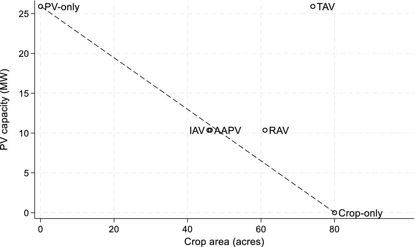
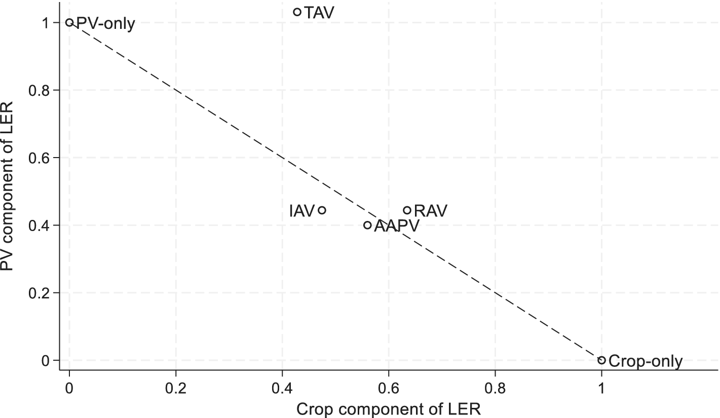
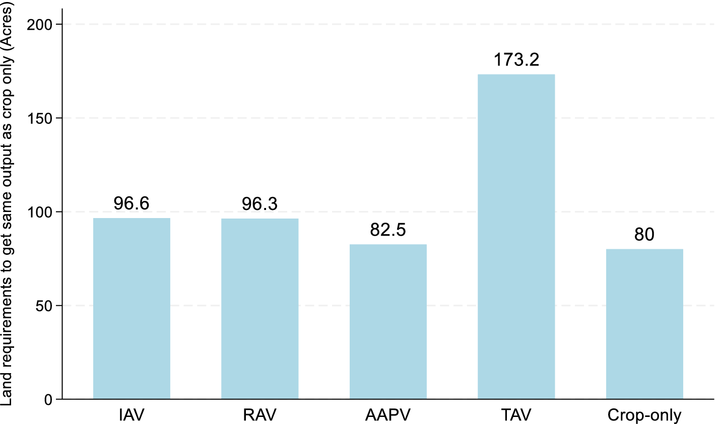
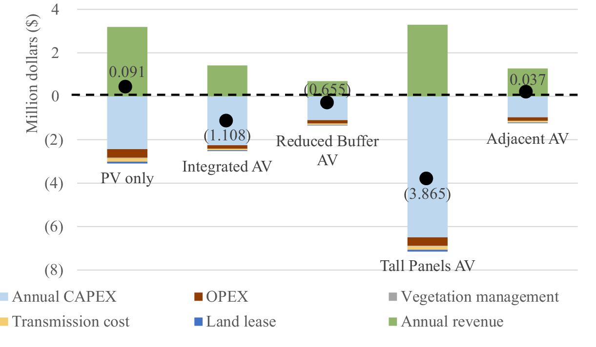
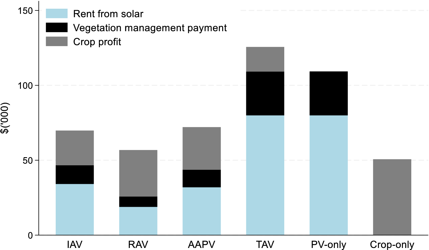
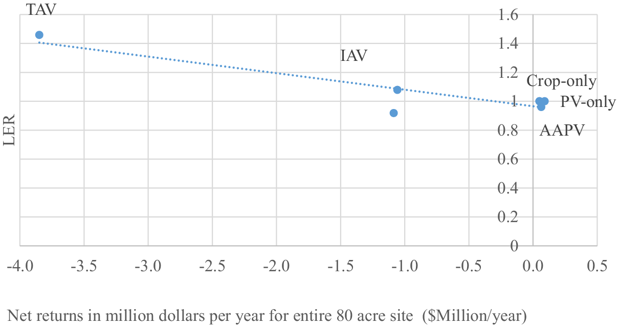
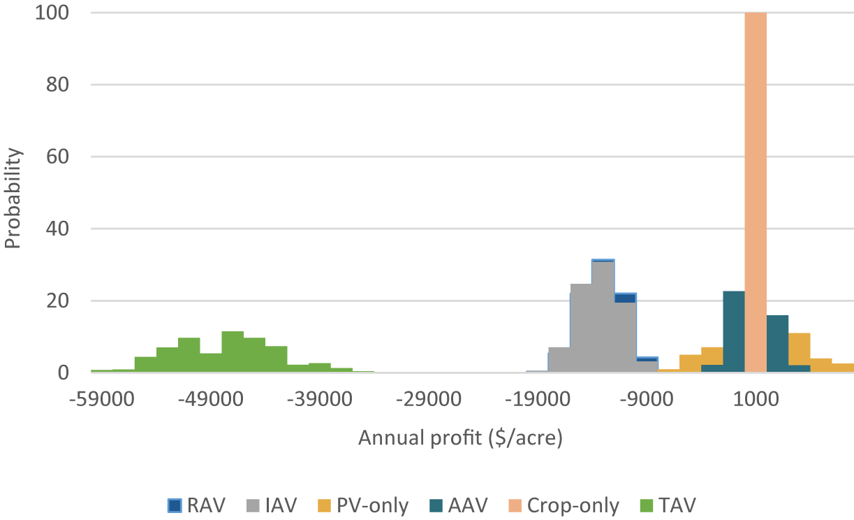
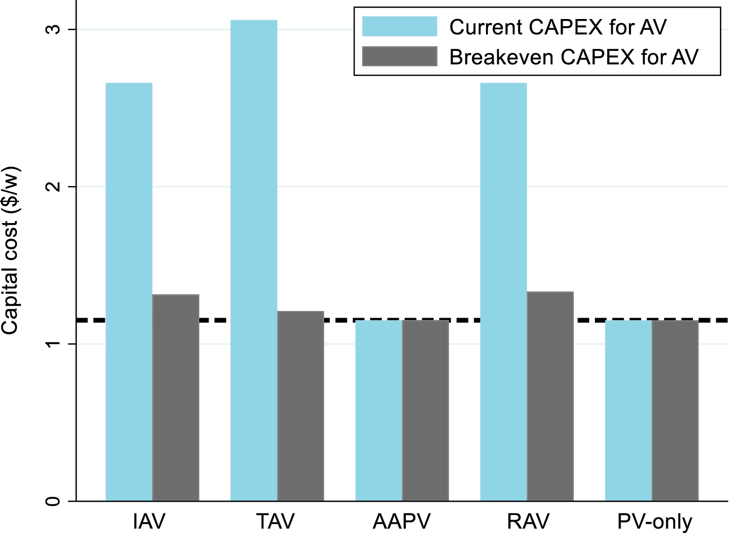
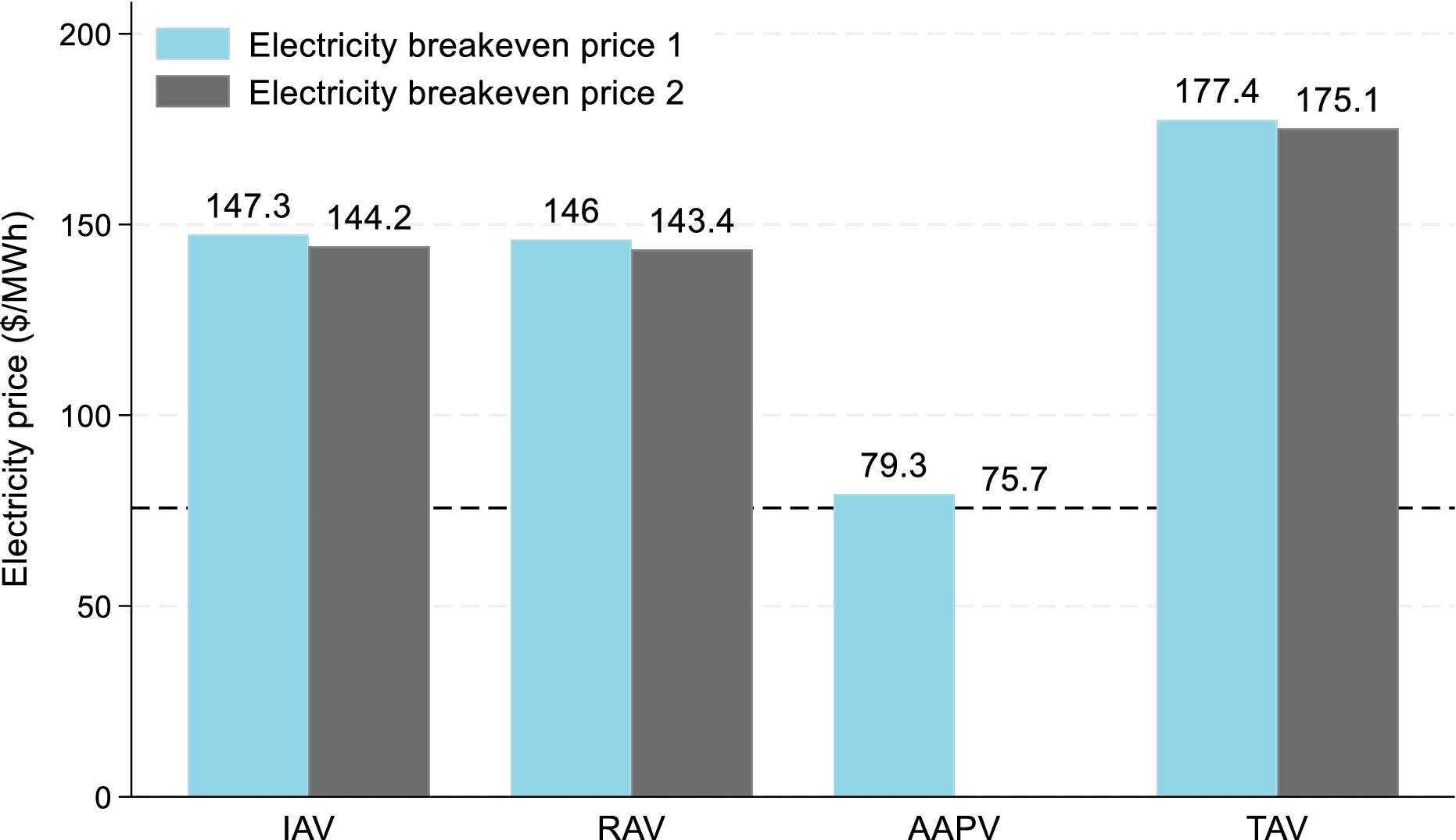
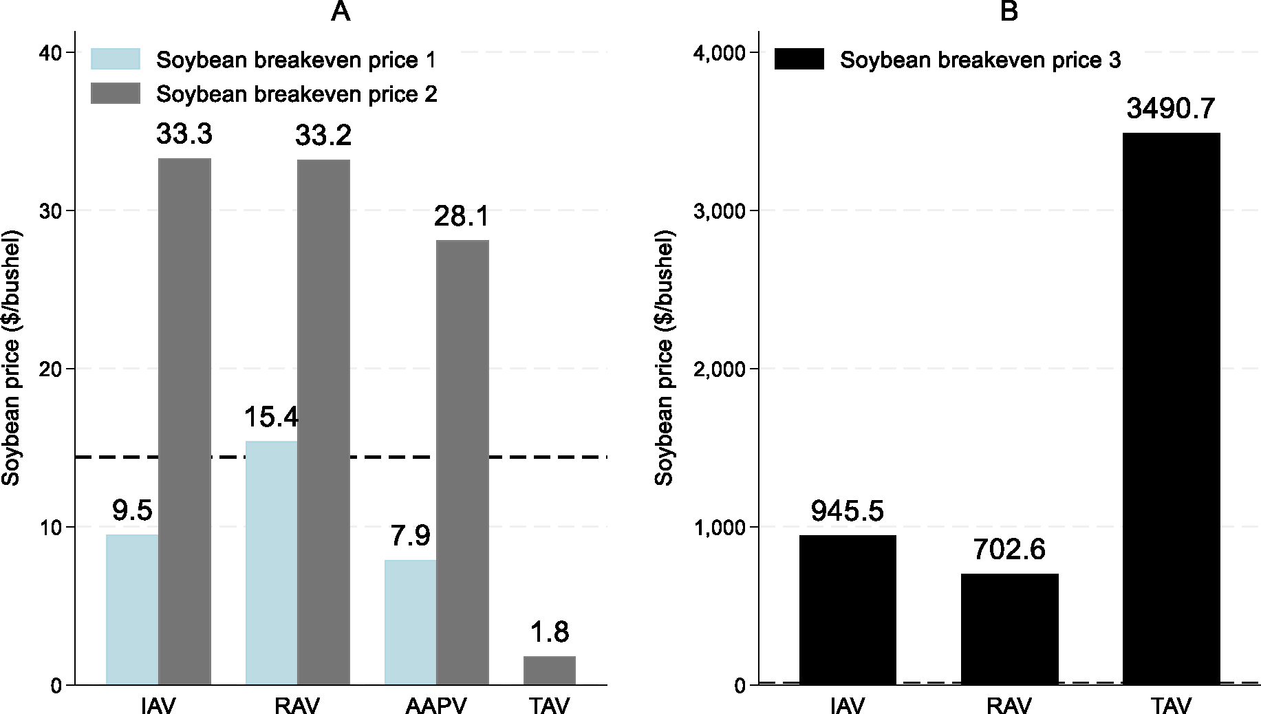


 Open access

