

Introduction
As poikilotherms, insect development rates and thresholds are temperature dependent (Taylor Reference Taylor1981). In seasonal environments evolved adaptations in these and related physiological traits, including diapause and quiescence, serve to synchronise developmental timing with local climates (Tauber and Tauber Reference Tauber and Tauber1976; Danks Reference Danks1987), and to enhance mate-finding and host plant feeding (Forrest and James Reference Forrest and James2011; Li et al. Reference Li, Johnson and Banks Sobota2011). For species that inhabit highly seasonal and cold environments, these strategies can also reduce the probability that lifestages vulnerable to cold-induced mortality are present during winter. Due to their significant influence on population success, thermally dependent fitness traits commonly vary with environmental conditions along latitudinal gradients, particularly in species with extensive distributions (Deutsch et al. Reference Deutsch, Tewksbury, Huey, Sheldon, Ghalambor, Haak and Martin2008). Understanding intraspecific trait variability is key to predicting population responses in a changing climate.
Mountain pine beetle (Dendroctonus ponderosae Hopkins; Coleoptera: Curculionidae: Scolytinae) is a bark beetle native to mountainous areas of western North America with an expansive distribution that ranges from Baja Norte, Mexico to northern British Columbia and Alberta, Canada (Cooke and Carroll Reference Cooke and Carroll2017; Dowle et al. Reference Dowle, Bracewell, Pfrender, Mock, Bentz and Ragland2017). Mountain pine beetle feeds on, reproduces in, and, when populations are at outbreak levels, kills pine (Pinus Linnaeus; Pinaceae) trees. Mountain pine beetle was responsible for 5.2 million hectare of pine mortality in the western United States of America between 1997 and 2012 (Hicke et al. Reference Hicke, Meddens and Kolden2016). In addition to the availability of suitable host trees, weather that supports appropriate seasonal timing and synchronous adult emergence are essential for population outbreaks (Logan and Bentz Reference Logan and Bentz1999; Safranyik and Carroll Reference Safranyik and Carroll2006). Pines have evolved resins and other defensive compounds to resist attack (Franceschi et al. Reference Franceschi, Krokene, Christiansen and Krekling2005; Boone et al. Reference Boone, Aukema, Bohlmann, Carroll and Raffa2011), and synchronous adult emergence facilitates a mass attack on individual trees that can occur more quickly than a tree can mobilise its defenses (Berryman et al. Reference Berryman, Dennis, Raffa and Stenseth1985). Successful attacks on the largest and often better defended trees with the thickest phloem (i.e., food for developing larvae) can lead to increased offspring and ultimately a population outbreak (Raffa et al. Reference Raffa, Aukema, Bentz, Carroll, Hicke, Turner and Romme2008). In northern United States of America mountain pine beetle, synchronous adult emergence is achieved by temperature-dependent physiological strategies including a facultative prepupal diapause (Bentz and Hansen Reference Bentz and Hansen2017) and lifestage-specific developmental rates and thresholds (Bentz et al. Reference Bentz, Logan and Amman1991; Powell and Logan Reference Powell and Logan2005; Régnière et al. Reference Régnière, Powell, Bentz and Nealis2012).
In addition to facilitating synchronicity in lifestage timing, evolved temperature-dependent physiological strategies control the time required to complete a generation and subsequently the number of generations that can be completed annually (i.e., voltinism). A lifecycle that is appropriately timed and results in one generation per year is considered univoltine, two generations in a single year is considered bivoltine, and semivoltine generations occur when two years are required for a single generation. Mountain pine beetle adult emergence typically occurs in mid to late summer across its range and univoltinism is considered the most optimal strategy (Logan and Bentz Reference Logan and Bentz1999; Safranyik and Carroll Reference Safranyik and Carroll2006). Bivoltinism has not been observed at the warmest or most southern extent of the current mountain pine beetle range in the United States of America (Hopkins Reference Hopkins1909; Bentz and Powell Reference Bentz and Powell2014; Bentz et al. Reference Bentz, Vandygriff, Jensen, Coleman, Maloney and Smith2014; B.J.B. unpublished data). A combination of univoltine and semivoltine strategies, however, can be found in outbreak-level populations at the highest elevations (Bentz et al. Reference Bentz, Vandygriff, Jensen, Coleman, Maloney and Smith2014), demonstrating that semivoltinism is a viable strategy in the coldest areas (Weed et al. Reference Weed, Bentz, Ayers and Holmes2015).
The pervasiveness of univoltinism found across the range of mountain pine beetle in the western United States of America masks thermally dependent strategies that evolved as a result of climatic differences across latitudes (Bentz et al. Reference Bentz, Vandygriff, Jensen, Coleman, Maloney and Smith2014), as revealed in common garden studies. Median generation time of southern United States of America populations was significantly longer than mountain pine beetle from northern United States of America populations when reared at the same constant temperature (Bentz et al. Reference Bentz, Logan and Vandygriff2001; Bentz et al. Reference Bentz, Bracewell, Mock and Pfrender2011; Bracewell et al. Reference Bracewell, Pfrender, Mock and Bentz2013). Countergradient variation, a type of phenotypic plasticity wherein the evolutionary response to a gradient is opposite of the ecological response, is not uncommon in species with large geographic ranges (Conover and Schultz Reference Conover and Schultz1995). The observed longer generation time in southern mountain pine beetle is likely a result of selection pressure to maintain univoltinism despite a warmer climate. To predict the impact of continued climate warming on population success, an understanding of the strategies and lifestages responsible for developmental differences between southern and northern mountain pine beetle populations is critical.
Our goal was to describe temperature-dependent lifestage-specific developmental times and thresholds for a southern United States of America mountain pine beetle population. We then compare our results with previously described developmental data for a northern United States of America population (Régnière et al. Reference Régnière, Powell, Bentz and Nealis2012). Using maximum posterior likelihood estimation, we fit observed data on time to complete each lifestage across a range of temperatures to the same seven parameter rate function used by Régnière et al. (Reference Régnière, Powell, Bentz and Nealis2012), adding a Bayesian prior to the procedure to increase stability in the model fits. We also used transfer treatments to facilitate timely data collection and increase survival at extreme temperatures, and developed a method of assessing the reliability and effectiveness of those treatments. Our comparison of lifestage-specific thermal responses for northern and southern mountain pine beetle populations provides a platform for increased understanding of evolved developmental differences across latitudes, in addition to the development of a phenology model for southern populations that can be used in predicting range-wide population success in a changing climate.
Methods
Experimental materials and design
To obtain fresh phloem material to infest with mountain pine beetle parents from a southern population, one live, un-infested southwestern white pine (Pinus strobiformis Engelmann) was harvested on 3 May 2016 near Flagstaff, Arizona, United States of America (35.36272, −111.7439) and cut into 50–55 cm bolts. Bolts were transported to the United States Forest Service Rocky Mountain Research Station laboratory in Logan, Utah, United States of America and bolt ends were waxed (Gulf Wax, Roswell, Georgia, United States of America) to retain moisture and then stored at 0 °C for up to two months. Unmated adults for infesting the bolts of host tree material were acquired by harvesting a mountain pine beetle-infested southwestern white pine on 4 May 2016 near Flagstaff, Arizona (35.35506, −111.6132). The infested tree was cut into bolts 45–50 cm long and transported to the Rocky Mountain Research Station laboratory in Logan, Utah. Bolts ends were waxed to retain moisture and stored at 0 °C when not used to produce brood. Eight bolts from the infested tree were immediately placed in incubators (Percival Scientific, Perry, Iowa, United States of America) (four bolts per incubator) at ~20 °C to facilitate brood development and adult emergence. Adults were collected daily and kept at 4 °C in Petri dishes for one to seven days before use. Moistened filter paper was placed in each dish to reduce desiccation. Beetles were sexed using secondary sex characteristics on the seventh tergite (Lyon Reference Lyon1958). Voucher specimens are stored at the Rocky Mountain Research Station Logan Forestry Sciences Laboratory (Logan, Utah, United States of America) and Utah State University Insect Collection (Logan, Utah, United States of America).
Phloem sandwiches were used to monitor lifestage-specific development following methods found in Bentz et al. (Reference Bentz, Logan and Amman1991) and Hansen et al. (Reference Hansen, Bentz and Turner2001). Sandwiches were initiated with eggs, and development of each individual was monitored on a daily basis until the adult stage was reached or mortality occurred. To obtain eggs, several un-infested bolts were manually infested with male/female pairs by inserting first a female then a male into holes drilled vertically into the phloem. Wire mesh screen was placed over each hole to prevent parent beetle escape. The bolts were inverted and incubated at room temperature for 10–12 days before peeling the bark to expose egg galleries. Eggs were collected from three 1.5-cm gallery sections, starting with the most recently completed gallery, and eggs were considered to be one, two, or three days old, respectively, based on preliminary data on rate of gallery construction and oviposition (McManis Reference McManis2018).
To obtain phloem for sandwiches, the outer bark was stripped from several un-infested bolts with a sterilised draw knife. Phloem pieces were cut into six-inch squares using a sterilised knife and carefully peeled from the bolt. Peeled phloem squares were vacuum packed (FoodSaver; Sunbeam Products, Boca Raton, Florida, United States of America) and refrigerated for one to two days before use. Phloem sandwiches were assembled using tools sterilised in 95% ethanol to reduce contamination. On the cambial surface of the phloem, seven evenly spaced niches for eggs were cut along the centreline of the phloem parallel to the grain with a sterilised dissecting probe. For each phloem sandwich eggs of similar age were used (i.e., one, two, or three days old). Phloem containing eggs was placed between sterilised glass and sterilised plexiglass plates, with plexiglass against the bark side and glass against the cambial side with the eggs. These “sandwiches” were clamped on each edge and the edges secured with tape (Nexcare 3 M, St. Paul, Minnesota, United States of America) and parafilm (Bemis, Neenah, Wisconsin, United States of America).
Completed phloem sandwiches (hereafter, “plates”) were numbered and placed upright in racks in 26-cm-diameter plastic desiccators (Bel-Art SP Scienceware; Fisher Scientific, Pittsburg, Pennsylvania, United States of America), with a 5% sodium chloride solution in the bottom to maintain constant humidity (~ 93%), and the desiccators were placed in incubators. Individual eggs were numbered from 1–7 for each plate by writing on the glass next to the current location of the individual. There were seven plates per desiccator, and two desiccators per temperature, for a total of 98 individuals at each temperature, 10 °C, 15 °C, 20 °C, 25 °C, 27 °C, 28 °C, 29 °C, and 30 °C. Experimental temperatures were spread asymmetrically across the previously developed rate curve for a northern population (Régnière et al. Reference Régnière, Powell, Bentz and Nealis2012) to ensure sufficient data to resolve the upper and lower developmental thresholds. Because the slope of the development rate curve at temperatures lower than the expected optimal (~ 25 °C) is shallow, we included temperatures every 5 °C between 10 °C and 25 °C. Expecting a sudden sharp drop in development rate above the optimal, we included temperatures every 1 °C between 27 °C and 30 °C.
Plates were inspected under a dissecting microscope every 24 hours and larval head capsule width recorded. When present, discarded head capsule exuviae, indicating a recent moult to a new instar, was also recorded for each individual. In the absence of head capsule exuviae, increases in head capsule width of at least 0.5 mm between individual observations were recorded as advancement to the next instar. An individual was considered a pupa when a loss of larval body morphology and the presence of proto-wing structures were observed. An individual was considered an adult when adult structures were present (e.g., legs and elytra) and sclerotisation began (i.e., the individual turned from a creamy white to light brown). From these data, the number of days to complete each instar/lifestage at a particular temperature was calculated for each individual. Individuals that failed to complete a lifestage (i.e., died or were still alive at the end of the experiment) or transitioned between lifestages while hidden beneath the surface of the phloem (so that the exact date of transition was unknown) were included as censored data sensu (Régnière et al. Reference Régnière, Powell, Bentz and Nealis2012).
Transfer treatment implementation
Based on estimates of development time from preliminary data, in addition to previously published data on a northern population (Régnière et al. Reference Régnière, Powell, Bentz and Nealis2012), total development time for individuals at or below 15 °C and above 27 °C would require an extended amount of time, in addition to the likelihood of reduced survival. To reduce these effects, we used transfer treatments. Transfer treatments assume that thermal history does not influence development time, and they increase the probability of observing lower and upper thermal thresholds (Régnière et al. Reference Régnière, Powell, Bentz and Nealis2012). In transfer treatments, plates spent part of the time at the treatment temperature and part of the time at 25 °C. Transfer treatments were used for 10 °C, 15 °C, 29 °C, and 30 °C and included 98 individuals (14 plates) per temperature.
For each lifestage, individuals were kept at the treatment temperature for approximately seven days before transfer to 25 °C. Seven days was chosen as a compromise between accelerating data collection and ensuring that, even where rates were lowest, a nontrivial amount of development for an individual (i.e., 10–15%) would be completed at the treatment temperature. If an individual in the plate had already advanced to the next lifestage, the plate was left at the treatment temperature for another seven days. Plates were transferred from 25 °C back to the treatment temperature one day after the most advanced individual completed the current lifestage. There were seven individuals per plate, and the individual in the most advanced lifestage was used to determine if and when a plate should be transferred. This insured that all individuals spent at least seven days per lifestage at the treatment temperature, although some individuals spent more time.
For comparison, a constant temperature control at 10 °C with 49 individuals that were not transferred was established. After 382 days, the majority of these individuals had not completed development to the pupal stage. Data on eggs, and first, second, and third instars were used to compare development time of transferred and nontransferred individuals at 10 °C.
Model development
Although Régnière et al. (Reference Régnière, Powell, Bentz and Nealis2012) used a lognormal error distribution for northern population data, a normal distribution was a better description of variability among southern individual development times/rates at a given temperature. Lognormal error is multiplicative and lower rates correspond to lower variance regardless of temperature (Régnière et al. Reference Régnière, Powell, Bentz and Nealis2012). Conversely, normal error is additive and does not scale with development times/rates and was a better fit to the variability among southern individuals. Using normally distributed error also allowed for the possibility that the upper and lower threshold of an individual may vary relative to the median threshold in the population, whereas lognormal error assumes fixed upper and lower developmental thresholds for all individuals.
For the nth individual, there is a mismatch (ε
n
) between the observed development rate and the modelled mean rate due to individual variation in rate, which we assumed to be normally distributed with variance
 $ \sigma ^{2} $
. Therefore the rate of development of an individual,
 $r_{n} (T,{\mib{\theta }} )$
, relates to the mean rate,
 $r_{o} (T,{\mib{\theta }} )$
, as
 $$r_{n} \left( {T,{\mib{\theta }} } \right){\equals}{\rm }r_{o} \left( {T,{\mib{\theta }} } \right){\plus}{\rm }{\epsilon}_{n} ,{\rm }{\epsilon}_{n} \,\sim\,{\rm }N\left( {0,{\rm }\sigma ^{2} } \right),$$
where T is temperature, θ a vector of parameters, and
 $r_{o} (T,{\mib{\theta }} )$
the rate function,
 $$\eqalignno{r\left( {T,{\mib{\theta }} } \right){\equals} \psi \left[ {e^{{\omega (T{\minus}T_{b} )}} {\minus}\left( {{{T_{m} {\minus}T} \over {T_{m} {\minus}{\rm }T_{b} }}} \right)e^{{{\minus}{{\omega \left( {T{\minus}T_{b} } \right)} \over {{\rm \Delta }_{b} }}}}} \right. \cr {\left.{\minus}\left( {{{T{\minus}T_{b} } \over {T_{m} {\minus}T_{b} }}} \right)e^{{\omega \left( {T_{m} {\minus}T_{b} } \right){\minus}{{T_{m} {\minus}T} \over {{\rm \Delta }_{m} }}}} \right]},$$
previously used by Régnière et al. (Reference Régnière, Powell, Bentz and Nealis2012). In this rate function, T
m
and T
b
correspond to the upper and lower temperature thresholds, respectively, and the remaining parameters are shape parameters. The observed development time, t
n
, of individual n at constant temperature (T) gives an observed rate,
 $r_{n} \left( {T,{\mib{\theta }} } \right){\equals} {1 \over {t_{n} }}$
, and therefore the likelihood of observing t
n
is,
 $$L_{n} {\equals}{\rm }{{e^{{{\minus}{\rm }{{\left( {r_{o} \left( {T,{\mib{\theta }} } \right){\minus}{1 \over {t_{n} }}} \right)^{2} } \over {2\sigma ^{2} }}}} } \over {\sqrt {2\pi \sigma ^{2} } }}.$$
The negative log likelihood for the single observation, t
n
, (after multiplying the numerator and denominator by
 $t_{n}^{2} $
) becomes
 $$NLL_{n} {\equals}{\rm }{{(r_{o} \left( {T,{\mib{\theta }} } \right)t_{n} {\minus}1)^{2} } \over {2\sigma ^{2} t_{n}^{2} }}{\plus}{1 \over 2}{\rm ln}\left( {2\pi \sigma ^{2} } \right).$$
Transfer treatment data
For individuals that were transferred between temperatures to accelerate development and increase survival, fitting their data to the rate curve was more complicated. Integrating equation (1) gives
 $$\smallint \limit_0^t r_{n} \left( {T,\theta } \right)dt{\equals}{\rm }\smallint \limit_0^t r_{o} \left( {T,\theta } \right)dt{\plus}\vint \limit_0^t {\epsilon}_{n} dt.$$
For an individual that spent some time (
 $t_{{n1}} $
) at a treatment temperature (T
1) and some time (
 $t_{{n2}} $
) at T
2 (25 °C) this results in
 $$ \smallint \limit \limit_0^{(t_{{n1}} {\plus}t_{{n2}} )} r_{o} \left( {T,\theta } \right)dt{\equals}{\rm }r_{o} \left( {T_{1} ,\theta } \right)t_{{n1}} {\plus}r_{o} \left( {T_{2} ,\theta } \right)t_{{n2}} .$$
The integral from 0 to time of completion is always one:
 $$\mathop \smallint \limit_0^{(t_{{n1}} {\plus}t_{{n2}} )} r_{n} \left( {T,\theta } \right)dt{\equals}1,$$
and therefore
 $$1{\equals}r_{o} \left( {T_{1} ,\theta } \right)t_{{n1}} {\plus}r_{o} \left( {T_{2} ,\theta } \right)t_{{n2}} {\plus}{\epsilon}_{n} \left( {t_{{n1}} {\plus}t_{{n2}} } \right).$$
Solving for ε
n
and using
 ${\epsilon}_{n} \,\sim\, N(0, \sigma ^{2} )$
, the negative log likelihood for observing
 $(t_{{n1}} {\plus}t_{{n2}} )$
becomes
 $$\eqalignno {NLL_{n} {\equals} {\rm }{{\left( {r_{o} \left( {T_{1} ,\theta } \right)t_{{n1}} {\plus}r_{o} \left( {T_{2} ,\theta } \right)t_{{n2}} {\minus}1} \right)^{2} } \over {2\sigma ^{2} (t_{{n1}} {\plus}t_{{n2}} )^{2} }}\cr {\plus}{1 \over 2}{\rm ln}(2\pi \sigma ^{2} ).$$
Testing consistency of transfer treatment data
Developmental rates for transferred and control individuals at 10 °C were compared based on developmental deviance. Developmental deviance (
 $\Delta _{n} $
) is a measure of how observed developmental time for an individual differs from the median time in a particular lifestage. For individuals in a transfer treatment being moved between 10 °C and 25 °C, we first calculated the median rate of development at 10 °C,
 $R_{{10}} $
, using observed development rates for individuals at a constant 10 °C, and the median rate of development at 25 °C,
 $R_{{25}} $
, using observed development rates for individuals at a constant 25 °C. The
 $\Delta _{n} $
for an individual is calculated as
 $$\Delta _{n} {\rm }{\equals}t_{{10}} R_{{10}} {\plus}t_{{25}} R_{{25}} ,$$
where t
10 and t
25 are time spent at 10 °C and 25 °C, respectively. The
 $\Delta _{n} $
for individuals at a constant 10 °C who were not transferred is calculated the same way, except
 $t_{{25}} {\equals}0,$
so
 $$\Delta _{n} {\rm }{\equals}t_{{10}} R_{{10}} .$$
If development rate is not affected by thermal history of an individual, then the distributions of
 $\Delta _{n} $
values for individuals at a constant 10 °C and transferred individuals will not be significantly different. If development rate is affected by thermal history, then there will be a significant difference in the
 $\Delta _{n} $
values between treatment groups. Because sample sizes were relatively small and somewhat skewed, we used a nonparametric Wilcox Rank-Sum test (W) to compare groups (R Core Team 2015).
Censored data
Censored data represents individuals who failed to complete their current lifestage while data collection was ongoing or transitioned between lifestages while unobservable beneath the phloem such that the exact duration of the lifestage was unknown. Therefore, their total development time is at least as long as the observation time, but could have been longer. The probability (P) the observed time for a censored data point is less than the mean development time for that temperature is
 $$\eqalignno {P\left( {t_{n} \,\lt\,{1 \over {r_{o} \left( {T,\theta } \right)}}} \right) {\equals}P\left( {r_{o} \left( {T,\theta } \right)t_{n} \,\lt\,1} \right)\cr {\equals}P\left( {r_{o} \left( {T,\theta } \right)t_{n} {\minus}1\,\lt\,0} \right).$$
Since
 $1{\minus}r_{o} \left( {T,\theta } \right)t_{n} {\equals}{\epsilon}_{n} t_{n} $
and
 ${\epsilon}_{n} t_{n} $
~
 $N(0,\sigma ^{2} t_{n}^{2} )$
,
 $$P\left( {r_{o} \left( {T,\theta } \right)t_{n} {\minus}1\,\lt\,0} \right){\equals}F\left( {r_{o} \left( {T,\theta } \right)t_{n} ;\,{\rm }\sigma ^{2} t_{n}^{2} } \right),$$
where F is the normal cumulative density function with variance
 $\sigma ^{2} t_{n}^{2} $
. The negative log likelihood for a censored observation, t
n
, is then
 $$NLL_{n} {\equals}{\rm }{\minus}{\rm ln}\left[ {F\left( {r_{o} \left( {T,\theta } \right)t_{n} ;\,{\rm }\sigma ^{2} t_{n}^{2} } \right)} \right].$$
Adding a Bayesian prior to the negative log likelihood
A Bayesian prior was used to improve the stability of the fit for upper and lower threshold parameters. This weights the maximum likelihood fit using prior information and confidence in the prior. According to Bayes’ Theorem, the posterior distribution of the vector of parameters, θ, satisfies
 $$P\left( {{\mib{\theta }} {\rm \,\mid\,}t_{n} } \right){\equals}{\rm }{1 \over {P(t_{n} )}}{\rm }P\left( {t_{n} {\rm \,\mid\,}{\mib{\theta }} } \right)P({\mib{\theta }} ).$$
In this expression
 $P\left( {t_{n} {\rm \,\mid\,}{\mib{\theta }} } \right)$
is the likelihood, P(θ) is a prior distribution of the parameters and
 $P(t_{n} )$
an unknown constant that can be ignored. For example, assuming the prior distribution of the upper threshold (T
u
) is normal we can write the posterior likelihood as
 $$P\left( {T_{u} } \right){\equals}{\rm }e^{{{\minus}NLL\left( {{\mib{\theta }} \,\mid\,t_{n} } \right)}} \left( {{{e^{{{\minus}{\rm }{{\left( {T_{u} {\minus}U} \right)^{2} } \over {2\sigma _{u}^{2} }}}} } \over {\sqrt {2\pi \sigma _{u}^{2} } }}} \right),$$
where U and
 $\sigma _{u}^{2} $
are the mean and variance of the prior distribution. The posterior probability of observing t
n
is therefore
 $$P\left( {t_{n} } \right)\propto e^{{{\minus}NLL\left( {{\mib{\theta }} {\rm \,\mid\,}t_{n} } \right)}} P\left( {T_{u} } \right)P(T_{l} ),$$
where
 $P\left( {T_{u} } \right)$
and
 $P\left( {T_{l} } \right)$
are, respectively, the prior probability of particular upper and lower thresholds. Assuming
 $T_{u} $
~Normal
 $(U,\sigma _{u}^{2} )$
and
 $T_{l} $
~Normal
 $(L,\sigma _{l}^{2} )$
, the negative log posterior (NLP) is
 $$\eqalignno {{\rm NLP}\left( {{\mib{\theta }} \mid t_{n} } \right){\equals} {\rm NLL}\left( {{\mib{\theta }} \mid t_{n} } \right){\plus}{\rm }{{\left( {T_{u} {\minus}U} \right)^{2} } \over {2\sigma _{u}^{2} }}\cr {\plus}{{\left( {T_{l} {\minus}L} \right)^{2} } \over {2\sigma _{l}^{2} }}{\plus}K.$$
Here K is a constant which is independent of parameter values. Prior means for the upper thresholds were chosen based on high observed mortality in the data at 30 °C, and prior variances were set at
 $\sigma _{u}^{2} $
=0.125 and
 $\sigma _{l}^{2} $
=0.50, reflecting the differing steepness of the rate curves approaching upper and lower thresholds. Where consistent with our data, the lower threshold means for the northern population (Régnière et al. Reference Régnière, Powell, Bentz and Nealis2012) were used as priors for the southern population. If a fit generated by minimising the negative log posterior resulted in a steep drop off in the curve unsupported by our data, the prior mean was stepped down by 0.5 °C up to six times (at most a 3 °C decrease), the fit was rerun, and the parameters associated with the lowest negative log posterior was kept.
Descriptive statistics and pairwise comparison of observed developmental times
Using our data for the southern population and data for the northern population published in Régnière et al. (Reference Régnière, Powell, Bentz and Nealis2012), we compared observed developmental time in each population for egg, larva, and pupa at temperatures used in both studies (i.e., 10 °C, 20 °C, 25 °C, 27 °C). Data were analysed using a generalised linear model with a Poisson distribution (SAS version 9.4; SAS Institute, Cary, North Carolina, United States of America). Posthoc pairwise comparisons were tested with a Tukey–Kramer adjustment for multiple comparisons. We tested for size differences between the fourth instar with and without a fifth instar using a similar analyses based on a normal distribution.
Results
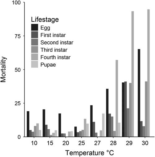
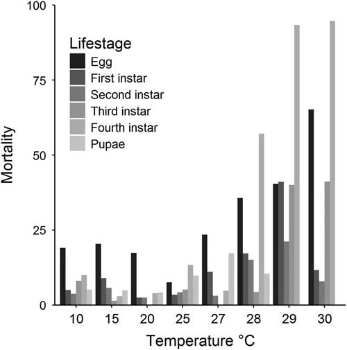
When individuals across all treatments were considered, mortality was greatest in the fourth instar (35%) and egg (29%). Mortality for all lifestages was lowest at 20 °C, and no individuals survived the pupal stage at 29 °C or 30 °C (Fig. 1). Although four instars have historically been described for mountain pine beetle (Logan et al. Reference Logan, Bentz, Vandygriff and Turner1998; Rosenberger et al. Reference Rosenberger, Venette and Aukema2018), Myrholm and Langor (Reference Myrholm and Langor2016) recently observed individuals with up to seven instars. We observed a fifth instar in 57 individuals (~ 14% of fourth instar individuals) at temperatures ≥15 °C. Headcapsule size of fifth instar (mean=1.39±0.09, n=51) was larger than the size of fourth instar (mean=1.26±0.08, n=348) (χ 2=101.23, P<0.0001). A headcapsule size was not measured for those individuals inappropriately oriented within phloem sandwiches. Of those individuals with a fifth instar, size of the fourth instar (mean=1.16±0.08, n=48) was smaller than fourth instars that did not moult to a fifth instar (mean=1.27±0.07, n=300) (χ 2=32.50, P<0.0001). Due to limited data, model parameters for a fifth instar could not be estimated.
Proportion mortality of southern population mountain pine beetle lifestages in phloem sandwiches at a range of constant temperatures (°C) throughout the experimental period.
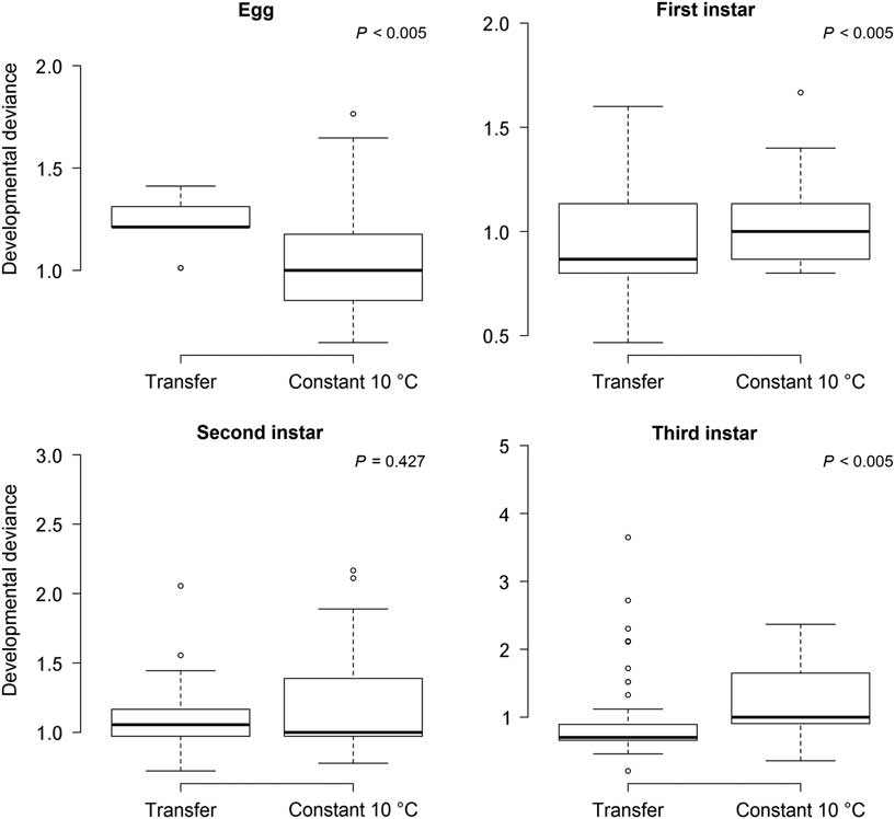
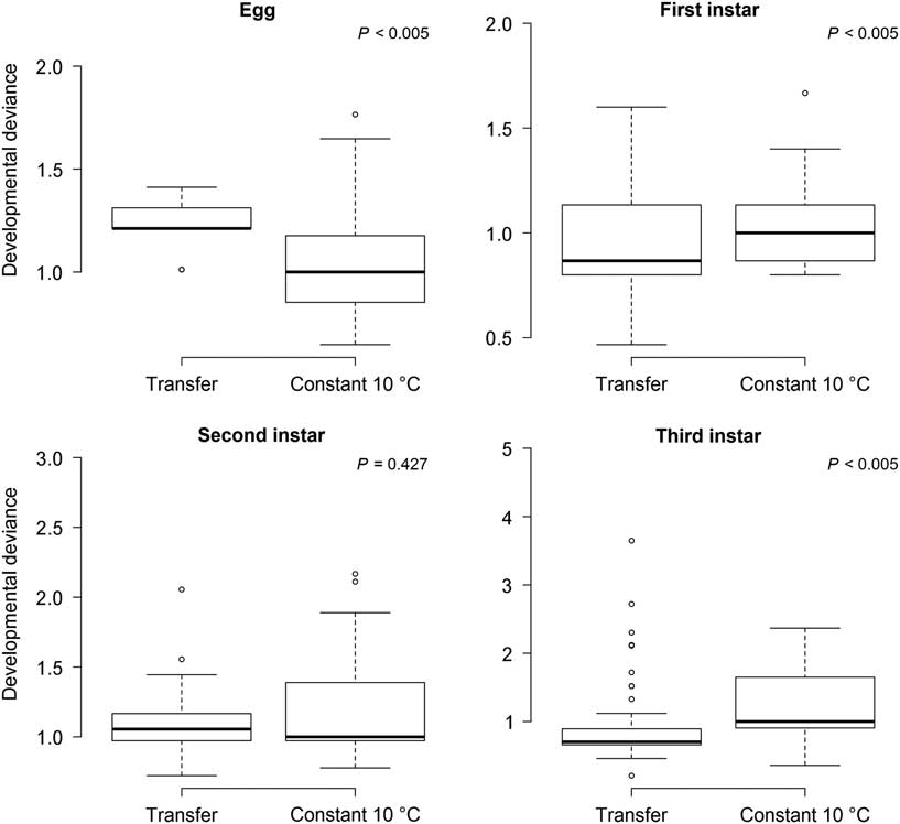
Developmental deviance, and therefore developmental rates, did not differ significantly for second instars that were either transferred from 10 °C to 25 °C or kept at a constant 10 °C (P=0.427). However, developmental deviance of eggs, first, and third instars were significantly different between transferred individuals and those kept at constant 10 °C (Fig. 2). We also observed reduced variability among transferred eggs, relative to eggs kept at a constant temperature (Fig. 2). There was insufficient constant temperature data to test for developmental differences between transferred and nontransferred individuals in the fourth instar, and subsequently pupa, because the majority of nontransferred fourth instars held at a constant 10 °C did not pupate. In contrast, a majority of the individuals transferred between 10 °C and 25 °C did pupate. Differences in pupation rates between transferred and nontransferred individuals are most likely a result of prepupal facultative diapause development that is sped up with warm temperatures (Bentz and Hansen Reference Bentz and Hansen2017). Due to observed differences, model fits were performed separately for temperature data with and without transfers for all stages except second instar.
Comparison of developmental deviance for individual eggs and first, second, and third instars in transfer treatments (i.e., transferred between 10 °C and 25 °C) versus a constant temperature control at 10 °C. Based on a Wilcoxon rank-sum test, transferred individuals developed significantly differently than individuals at a constant 10 °C in eggs (W=2100, P<0.005), and first (W=684.5, P=0.005) and third (W=353, P=0.005) instars. Boxes represent the third and first quartile (25th and 75th percentiles), whiskers extend up to 1.5 times the interquartile range from the top (bottom) of the box to the furthest data point, and the midline is the median.
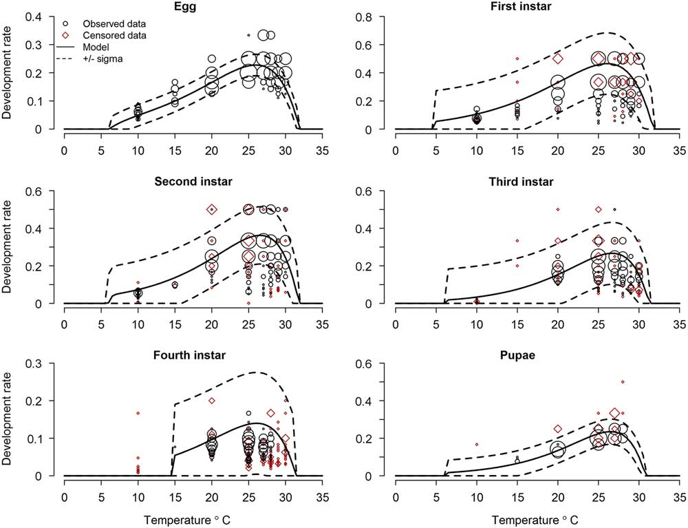
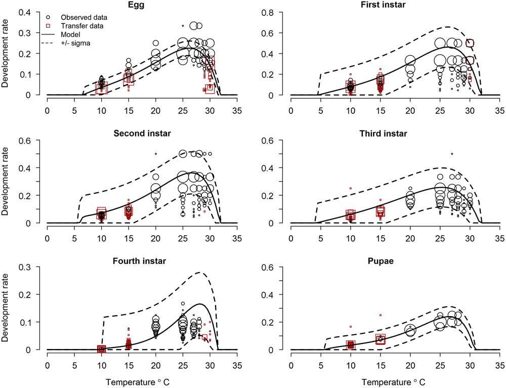
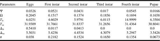
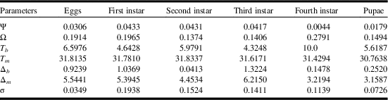
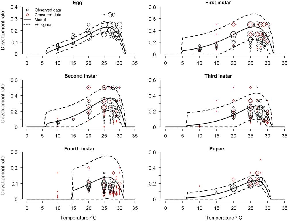
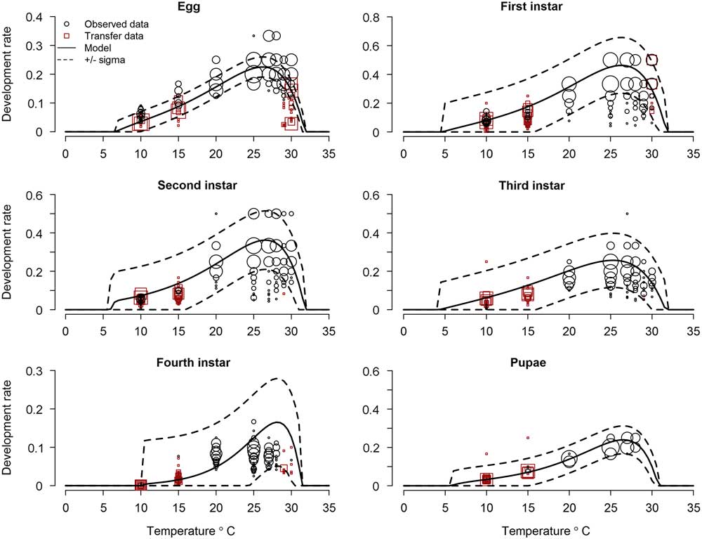
Using constant temperature and censored data (i.e., no transfer data), estimated parameters from the fit to equation (2) differed among lifestages (Table 1). In particular, the lower developmental threshold (T b ) for the fourth instar was estimated to be substantially higher (~ 15 °C) than all other life stages which ranged from ~ 4.6 °C to 6.3 °C (Table 1). The estimated upper developmental thresholds (T m ) were similar among lifestages and ranged from 30.8 °C to 31.9 °C. Optimal developmental rate was estimated to be between 24.8 °C and 26.5 °C for all lifestages (Fig. 3). At the optimal rate, first instars developed approximately twice as fast as eggs, third instars and pupae, and almost four times as fast as fourth instars. When data on individuals that were transferred among temperatures were included in parameter estimation, predicted development rates differed slightly from fits using constant temperature data, particularly in the fourth instar (Table 2; Fig. 4). Fourth instars exposed to 25 °C during part of their development (i.e., a transfer treatment) had positive development at temperatures ≤ 15 °C (Fig. 4) in contrast to fourth instars that were kept at a constant 10 °C or 15 °C, where no development was observed (Fig. 3).
Model-predicted and observed lifestage-specific developmental rates for a southern mountain pine beetle population based on constant temperature and censored data. “Censored” data represent individuals that did not complete the lifestage at a given temperature. Data for the fourth instar includes prepupal rates. All point sizes are on a log scale, with larger points corresponding to more highly repeated observations. Dashed lines are ± 1 sigma (standard deviation), the variance parameter associated with model fit. Note differences among plots in y-axis scale.
Model-predicted and observed lifestage-specific developmental rates for a southern mountain pine beetle population based on constant temperature and transfer data. “Transfer” data represent individuals that were transferred between the treatment temperature and a constant 25 °C. Data for the fourth instar includes prepupal rates. All point sizes are on a log scale, with larger points corresponding to more highly repeated observations. Dashed lines are ± 1 sigma (standard deviation), the variance parameter associated with model fit. Note differences among plots in y-axis scale.
Lifestage-specific parameters for the rate curve (equation 2) for a southern mountain pine beetle population using constant temperature data and censored data (see Fig. 3).

Notes: Data from transfer treatments was excluded from the model fits for eggs, first instar, third instar, and fourth instar. T b and T m are lower and upper thresholds for development, ∆b and ∆m are the width of thermal transitions from normal to negligible development at the lower and upper thresholds, ω describes the expected exponential acceleration of rate with temperature, ψ is proportional to the maximum development rate, and σ is the variance parameter (standard deviation).
Lifestage-specific parameters for the rate curve (equation 2) for a southern mountain pine beetle population including constant temperature data and data from transfer treatments (see Fig. 4).
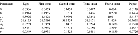
Notes: Second instar parameters are equivalent to those in Table 1 because there were no differences between transfer and constant temperature treatments. T b and T m are lower and upper thresholds for development, ∆b and ∆m are the width of thermal transitions from normal to negligible development at the lower and upper thresholds, ω describes the expected exponential acceleration of rate with temperature, ψ is proportional to the maximum development rate, and σ is the variance parameter (standard deviation).
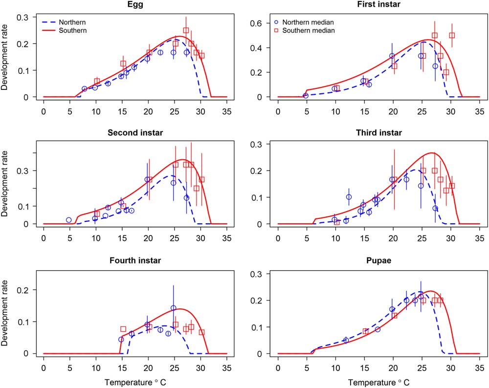
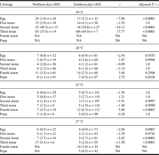
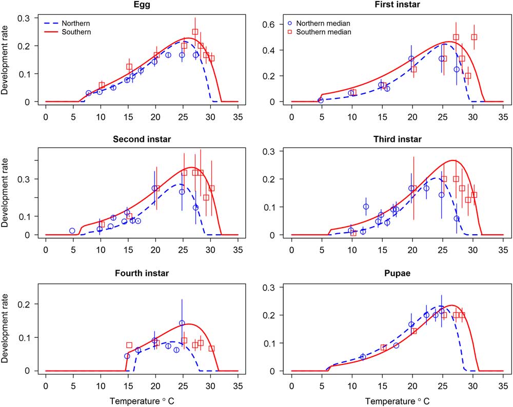
We were interested in comparing lifestage-specific observed developmental times and fitted rate curves of the southern population with those previously described for a northern population (Bentz et al. Reference Bentz, Logan and Amman1991; Régnière et al. Reference Régnière, Powell, Bentz and Nealis2012; Bentz and Powell Reference Bentz and Powell2014). The same phloem sandwich methodology was used to collect data for both populations. At a constant 10 °C, observed development time of southern population eggs and second instars was faster than northern individuals in the same lifestages, and southern third instars developed slower than northern third instars (Table 3). No individuals in either population completed fourth instar development (i.e., pupated) at 10 °C without some period of development at a warmer temperature. There were no significant differences in observed development time between the populations in any lifestage at 20 °C (Table 3). At 25 °C southern fourth instars developed significantly slower than northern fourth instars, and at 27 °C southern second and third instars developed faster than northern individuals (Table 3). When fitted development rate curves for each population were compared, using only not-transferred data, estimated upper thresholds were higher for southern compared to northern individuals across all lifestages (Fig. 5). Lower thresholds were similar between the populations in all lifestages except the fourth instar, where southern individuals developed at a lower temperature (Fig. 5). Estimated development rates of southern second and third instars were higher than northern second and third instars at all temperatures.
Comparison of predicted development rates of northern and southern mountain pine beetle populations. Southern population predictions were based on estimated parameters in the current study using nontransferred constant temperature and censored data (see Fig. 3). Northern population predictions were published in Régnière et al. (Reference Régnière, Powell, Bentz and Nealis2012; fig. 4), also using nontransferred constant temperature and censored data. Estimated upper (T m ) and lower (T b ) development thresholds for each population and lifestage are in Table 1. Also shown are the observed median development rates (±standard deviation) of each population at the common experimental temperatures (see Table 3 for observed development times).
Comparison of median development time (days) for southern (this study) and northern (Régnière et al. Reference Régnière, Powell, Bentz and Nealis2012) mountain pine beetle populations at a constant 10 °C, 20 °C, 25 °C, and 27 °C.

Notes: Shown are the median days, standard deviation (SD), sample size (n), and test results (z) using a generalised linear model with a Tukey’s posthoc multiple comparison (adjusted P) testing for differences between populations. No individuals in either population completed instar 4 or pupal development at a constant 10 °C.
Discussion
Our goal was to describe temperature-dependent lifestage-specific developmental times and thresholds for a southern mountain pine beetle population. We then compared these developmental data from a southern population with previously described developmental data for a northern population that was collected using the same phloem sandwich method (Régnière et al. Reference Régnière, Powell, Bentz and Nealis2012). Previous research showed that in common garden experiments, median generation time of a southern population was significantly longer (~ 73 days) than that of a northern population at 22 °C (Bracewell et al. Reference Bracewell, Pfrender, Mock and Bentz2013), and we were interested in identifying the lifestage(s) and evolved traits that may differ between the populations. Estimated upper developmental thresholds and optimal development rates were at slightly higher temperatures for southern compared to northern individuals across all lifestages. Although northern data was not collected at temperatures ≥ 28 °C, the slowing trend in northern individuals at 27 °C suggests optimal development occurs at slightly higher temperatures in southern individuals. Southern fourth instars that were not transferred to 25 °C during development pupated (i.e., completed the fourth instar) at a lower temperature than did northern fourth instars given the same treatment, a result also found by Bentz and Hansen (Reference Bentz and Hansen2017). Both populations have a facultative prepupal (i.e., last stage of the fourth instar) diapause, and induction can occur at higher temperatures in northern (15–17 °C) compared with southern populations (< 15 °C) (Bentz and Hansen Reference Bentz and Hansen2017). Southern fourth instars developed slower than northern fourth instars, but only significantly so at 25 °C. At all other temperatures and lifestages, southern individuals generally developed faster than northern individuals.
Given the longer total development time from egg through adult emergence of southern compared to northern individuals at a constant 22.5 °C (Bracewell et al. Reference Bracewell, Pfrender, Mock and Bentz2013), we hypothesised that selection would act on one or more lifestages to slow development rates and thereby maintain univoltinism despite warmer habitat temperatures. Although development was generally faster in southern individuals, our result that southern fourth instars developed slower (approximately five days) than northern fourth instars at 25 °C highlights that physiological aspects of the fourth instar may partially explain generation time differences between the populations. In addition to the lifestages monitored in our study, total development time as reported by Bracewell et al. (Reference Bracewell, Pfrender, Mock and Bentz2013) included oviposition and teneral (i.e., preemergent) adult development through emergence. McManis (Reference McManis2018) showed that oviposition is slightly slower in southern compared to northern mountain pine beetle (18.5 versus 12 days at 21 °C). This time difference, combined with the few days difference in fourth instar, contribute only marginally to the observed median difference of 73 days in total generation time. A potential additional explanation for differences in generation time observed by Bracewell et al. (Reference Bracewell, Pfrender, Mock and Bentz2013) is trait differences between the populations in the unstudied teneral adult stage. Differences in evolved traits such as adult development and maturation rates, and temperature thresholds for emergence from beneath the bark could result in differences in adult emergence timing and generation time. Because teneral adults feed on spores of fungal associates to obtain vital nutrients prior to emergence (Six and Paine Reference Six and Paine1998), differences in fungal acquisition or species composition could also play a role in developmental differences between the populations (Addison et al. Reference Addison, Powell, Bentz and Six2014).
A proportion of individuals (~ 14%) moulted to a fifth instar prior to pupation. Plasticity in the number of instars an insect may go through prior to pupation can be influenced by multiple environmental factors including temperature and food quality and quantity (Esperk et al. Reference Esperk, Tammaru and Nylin2007). Myrholm and Langor (Reference Myrholm and Langor2016) recently observed mountain pine beetles with up to seven instars, and the headcapsule sizes of the additional instars were between that of instar 3 and instar 4. They suggested that inadequate nutrition results in extra instars and that larvae must attain a threshold size to initiate metamorphosis (Nijhout Reference Nijhout1994). In constrast to Myrholm and Langor (Reference Myrholm and Langor2016), the size of the additional instar we observed was larger than the size of fourth instars, and therefore was the last instar prior to pupation. Moreover, individuals that moulted to a fifth instar were smaller as a fourth instar than were individuals that pupated following the fourth instar. Our results concur with Myrholm and Langor (Reference Myrholm and Langor2016) that a size threshold for pupation likely exists in mountain pine beetle, and that additional instars may serve as a compensatory mechanism in adverse conditions (Esperk et al. Reference Esperk, Tammaru and Nylin2007). Collectively, however, results suggest that the timing of supernumerary instars is not fixed.
Measuring insect development near thresholds can be difficult. We used temperature transfer treatments to increase survival at extreme temperatures and reduce the time required for measurements when development is slowed (Régnière et al. Reference Régnière, Powell, Bentz and Nealis2012). An assumption of transfer treatments is that past thermal history does not affect future developmental rate. We found that only second instars transferred between 10 °C and 25 °C met this assumption of no difference, with first and third instars developing faster than those kept at a constant 10 °C and transferred eggs developing more slowly. The apparent slowing of development in transferred eggs is likely due to the difficulty of accurately aging eggs, rather than the transfer treatment alone. For first and third instars, however, pulses of warm temperature (25 °C) during development at 10 °C resulted in slightly faster development. Future study is needed to determine if this effect is due to the relatively brief exposure of transferred individuals to their treatment temperature, or if it reflects more complex physiological processes.
A physiological-based description of the thermal response of an organism can provide a robust framework for making predictions of potential range shifts due to climatic changes. A major benefit of mechanistic, relative to statistical, models is that inherent biological behaviours can emerge. Our description of developmental responses of a southern United States of America mountain pine beetle population provide a foundation for incorporating evolved geographic variation in mountain pine beetle lifecycle timing into predictive models. Our findings suggest that future research should focus on physiological traits in the fourth instar and teneral adult lifestages to further our understanding of intraspecific fitness trait differences that drive population success across the expansive mountain pine beetle range.
Acknowledgements
The authors thank Jim Vandygriff and Matt Hansen for substantial assistance with data collection and help with experimental design and analysis. The authors also thank Luke Lemmon, Erika Eidson, and David Soderberg for assistance with data collection, and Monica Gaylord and John Anhold of the United States Department of Agriculture Forest Service Forest Health Protection Office, Flagstaff, Arizona and Dr. Rich Hofstetter of Northern Arizona University, Flagstaff, Arizona for assistance and research permissions. The authors acknowledge funding from the United States Department of Agriculture Forest Health Protection Special Technology Development Program R3-2015-04.