1 Introduction
The study of lateral migration of particles (solid particles, drops, bubbles and biological cells) is of immense importance because of its practical uses in microfluidic applications such as sorting and separation of particles, transport of biological cells and so on (Di Carlo et al. Reference Di Carlo, Irimia, Tompkins and Toner2007; Bhagat et al. Reference Bhagat, Bow, Hou, Tan, Han and Lim2010; Geislinger & Franke Reference Geislinger and Franke2013; Chen Reference Chen2014). Different mechanisms that have shown to cause the lateral migration of particles in the presence of background flows pertain to interface deformability (Goldsmith & Mason Reference Goldsmith and Mason1962; Chaffey, Brenner & Mason Reference Chaffey, Brenner and Mason1965; Karnis & Mason Reference Karnis and Mason1967; Haber & Hetsroni Reference Haber and Hetsroni1972; Wohl & Rubinow Reference Wohl and Rubinow1974; Stan et al. Reference Stan, Guglielmini, Ellerbee, Caviezel, Stone and Whitesides2011; Mandal, Bandopadhyay & Chakraborty Reference Mandal, Bandopadhyay and Chakraborty2015), fluid inertia (Ho & Leal Reference Ho and Leal1974; Mortazavi & Tryggvason Reference Mortazavi and Tryggvason2000; Chen et al. Reference Chen, Xue, Zhang, Hu, Jiang and Sun2014), non-Newtonian rheology (Chan & Leal Reference Chan and Leal1979; Mukherjee & Sarkar Reference Mukherjee and Sarkar2013, Reference Mukherjee and Sarkar2014) and Marangoni effects (Hanna & Vlahovska Reference Hanna and Vlahovska2010; Schwalbe et al. Reference Schwalbe, Phelan, Vlahovska and Hudson2011; Pak, Feng & Stone Reference Pak, Feng and Stone2014). Recently, the use of an external electric field to manipulate particles has been employed due to the convenience with which the electric field can be applied and modulated (Velev, Prevo & Bhatt Reference Velev, Prevo and Bhatt2003; Zeng & Korsmeyer Reference Zeng and Korsmeyer2004; Velev & Bhatt Reference Velev and Bhatt2006; Mcgrath, Jimenez & Bridle Reference Mcgrath, Jimenez and Bridle2014).
Electrohydrodynamics of drops and bubbles has been studied extensively in the existing literature. Starting from the pioneering work of Taylor (Reference Taylor1966), several authors have addressed the problem of deformation of neutrally buoyant, leaky dielectric drops in uniform and non-uniform electric fields (Torza, Cox & Mason Reference Torza, Cox and Mason1971; Ward & Homsy Reference Ward and Homsy2001, Reference Ward and Homsy2003, Reference Ward and Homsy2006; Feng & Scott Reference Feng and Scott2006; Vizika & Saville Reference Vizika and Saville2006; Lac & Homsy Reference Lac and Homsy2007; Supeene, Koch & Bhattacharjee Reference Supeene, Koch and Bhattacharjee2008; Thaokar Reference Thaokar2012; Lanauze, Walker & Khair Reference Lanauze, Walker and Khair2013; Zhang, Zahn & Lin Reference Zhang, Zahn and Lin2013; Deshmukh & Thaokar Reference Deshmukh and Thaokar2013). In these works, it was implicitly considered that the flow field does not affect the charge distribution at the drop surface and this assumption decouples the electric field from the flow field. As a non-trivial extension of the previously mentioned works, Feng (Reference Feng1999) demonstrated that the deformation is significantly altered by the surface-charge convection. A recent study shows that charge convection at the drop interface not only affects the steady-state deformation of the drop but also markedly alters the transient deformation behaviour of the drop (Lanauze, Walker & Khair Reference Lanauze, Walker and Khair2015). Therefore, one would expect that a background flow field may also significantly affect the drop dynamics by altering the interfacial charge distribution. However, only a few studies (Xu & Homsy Reference Xu and Homsy2006; Xu Reference Xu2007; Mahlmann & Papageorgiou Reference Mahlmann and Papageorgiou2009; Vlahovska Reference Vlahovska2011) have been reported in the existing literature that consider the electrohydrodynamic motion of a single drop or bubble in the presence of an imposed background flow. Xu & Homsy (Reference Xu and Homsy2006) have shown the influence of surface-charge convection and drop deformation on the velocity of a sedimenting leaky dielectric drop in the presence of uniform axial electric field for nearly spherical drop and small charge relaxation time scale. Later, Vlahovska (Reference Vlahovska2011) studied the drop dynamics in the presence of imposed shear flow and uniform electric field, and showed that the surface-charge convection alters the rotation rate of a highly viscous drop. The surface-charge convection also affects the shear viscosity and normal stress of a dilute emulsion containing drops as shown by Vlahovska (Reference Vlahovska2011). Mahlmann & Papageorgiou (Reference Mahlmann and Papageorgiou2009) have studied the effect of uniform electric field on the deformation and inclination angle of a drop in a confined shear flow using numerical simulations.
In the present work, our focus is to bring out the effect of surface-charge convection and interface deformation on the drop motion in the presence of an arbitrarily oriented uniform electric field. Generalizing the axisymmetric considerations of Xu & Homsy (Reference Xu and Homsy2006) concerning a sedimenting drop in the presence of a longitudinal electric field, we develop a three-dimensional formalism that aims at providing a unified framework for capturing non-trivial characteristics of drop migration in arbitrarily oriented uniform electric fields that have hitherto remained unaddressed. We analytically derive the velocity of a sedimenting drop and the associated electric and flow fields considering small interface deformation and small charge convection. We explicitly show the effect of charge convection and interface deformation on the drop velocity. We show the pivotal role of the tilt angle, which quantifies the angle between the direction of applied electric field and the direction of gravity, on the drop velocity. Quite remarkably, our results reveal a non-intuitive lateral (perpendicular to the direction of gravity) motion of the drop in the presence of a tilted electric field due to combined effect of charge convection and interface deformation. This lateral motion is fundamentally different from dielectrophoresis (in which non-uniformity in the applied electric field leads to motion of the polarizable particles) or electrophoresis (in which charged particles move in an electric field). The direction of lateral motion depends on the tilt angle and the ratios of the permittivities and conductivities of the two fluids. In sharp contrast to the case of a uniform electric field acting in the direction of gravity and contrary to common intuition, our results reveal the drop dynamics due to the coupling between the direction of the applied electric field, interface deformation and charge convection brought about by the drop sedimentation. We further validate experimentally the notion of lateral migration of the drop in the presence of a tilted electric field.
2 Problem formulation
We consider a Newtonian leaky dielectric drop of radius
 $a$
suspended in another Newtonian leaky dielectric fluid sedimenting under the influence of gravity acting in the positive
 $z$
-direction with an external electric field
 $(\boldsymbol{E}_{\infty })$
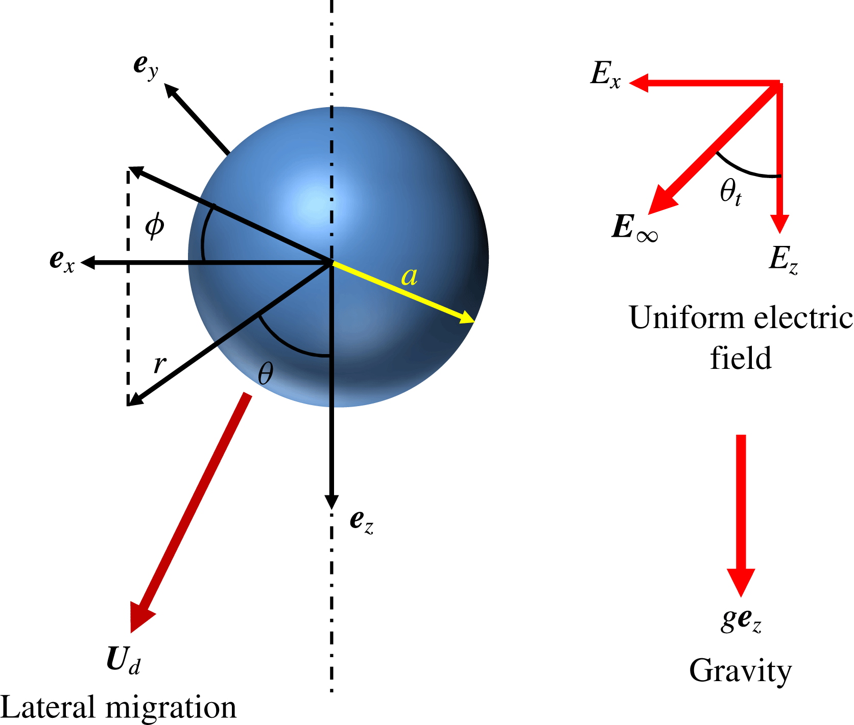
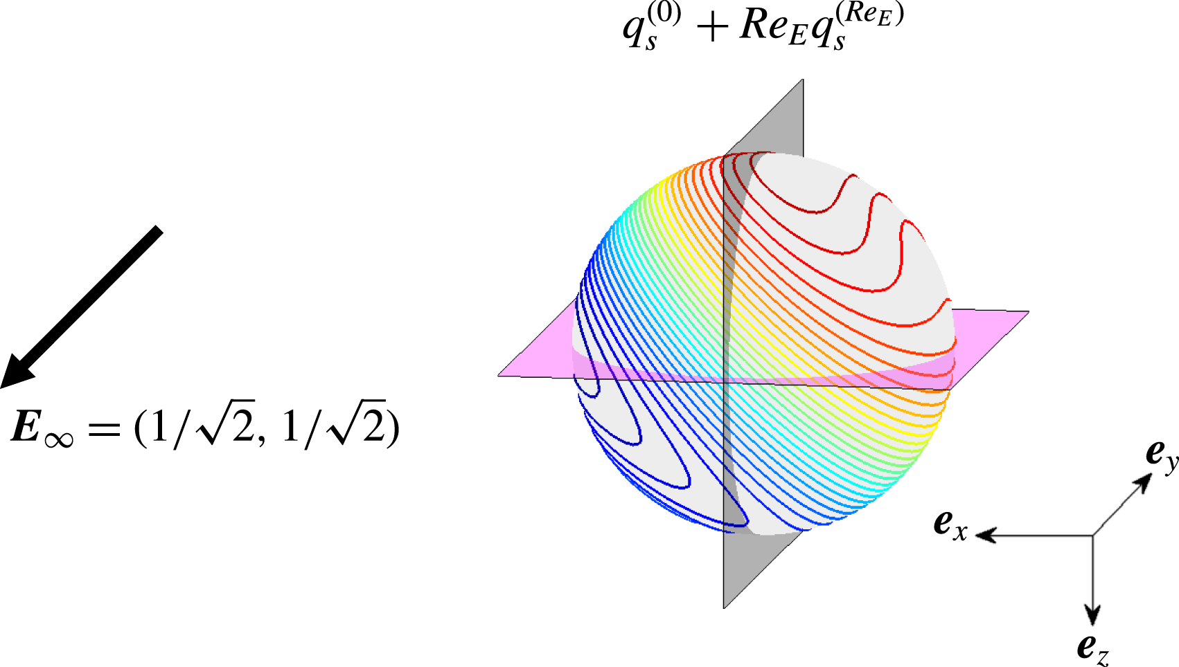
applied in an arbitrary direction (please refer to figure 1). The direction of application of the external electric field is specified by the tilt angle defined as
 ${\it\theta}_{t}=\tan ^{-1}(E_{x}/E_{z})$
. The centre of the spherical coordinate system
 $(r,{\it\theta},{\it\phi})$
is chosen at the centre of the drop which moves with a, so far unknown, velocity
 $\boldsymbol{U}_{d}$
. The density, viscosity, permittivity and conductivity of the inner fluid are denoted by
 ${\it\rho}_{i},{\it\mu}_{i},{\it\varepsilon}_{i}$
and
 ${\it\sigma}_{i}$
, respectively, while the same symbols with subscript
 $e$
denote the properties of the external fluid. The drop is immiscible in the suspending medium and the drop interface is characterized by a uniform surface tension
 ${\it\gamma}$
.
Schematic of a drop sedimenting in the presence of gravity and an imposed electric field
 $\boldsymbol{E}_{\infty }~(=E_{x}\boldsymbol{e}_{x}+E_{z}\boldsymbol{e}_{z})$
in an arbitrary direction. A spherical coordinate system
 $(r,{\it\theta},{\it\phi})$
is attached to the drop centroid.

We non-dimensionalize the length by the drop radius
 $a$
. In the absence of any applied electric field, the drop sediments in the
 $z$
-direction with a sedimenting velocity given by the Hadamard–Rybczynski velocity (Leal Reference Leal2007)
 $U_{HR}=(2/9)(ga^{2}({\it\rho}_{i}-{\it\rho}_{e})/{\it\mu}_{e})({\it\lambda}+1)/({\it\lambda}+2/3)$
, where
 ${\it\lambda}$
denotes the drop–medium viscosity ratio. Following the arguments by Xu & Homsy (Reference Xu and Homsy2006), we choose the characteristic velocity as
 $U_{HR}$
and, correspondingly, the characteristic hydrodynamic stress is taken as
 ${\bf\tau}_{ref}^{H}={\it\mu}_{e}U_{HR}/a$
. On similar lines, the electrical stress is non-dimensionalized by
 ${\bf\tau}_{ref}^{E}={\it\varepsilon}_{e}E_{ref}^{2}$
with
 $E_{ref}$
being the characteristic magnitude of the applied electric field. In the present work, all of the other properties are scaled by the properties of the outside fluid;
 ${\it\lambda}~(={\it\mu}_{i}/{\it\mu}_{e})$
denotes the viscosity ratio of the drop to medium,
 $R~(={\it\sigma}_{i}/{\it\sigma}_{e})$
denotes the conductivity ratio of the drop to medium and
 $S~(={\it\varepsilon}_{i}/{\it\varepsilon}_{e})$
denotes the permittivity ratio of the drop to medium. Under these considerations, we obtain the following important non-dimensional numbers (Xu & Homsy Reference Xu and Homsy2006; Vlahovska Reference Vlahovska2011):
 $Re=({\it\rho}_{e}aU_{HR})/{\it\mu}_{e}$
,
 $Ca=({\it\mu}_{e}U_{HR})/{\it\gamma}$
,
 $M=(a{\it\varepsilon}_{e}E_{ref}^{2})/{\it\mu}_{e}U_{HR}$
and
 $Re_{E}=({\it\varepsilon}_{e}U_{HR})/a{\it\sigma}_{e}$
. Here,
 $Re$
is the Reynolds number which signifies the relative magnitude of the inertia force as compared with the viscous force,
 $Ca$
is the Capillary number which signifies the relative magnitude of the viscous force as compared with the surface tension,
 $M$
is the Mason number which signifies the ratio of the electrical stress to the viscous stress and
 $Re_{E}$
is the electric Reynolds number which is the ratio of the charge relaxation timescale,
 ${\it\varepsilon}_{e}/{\it\sigma}_{e}$
, to the convective timescale,
 $a/U_{HR}$
. Using the physical properties pertinent to the reported experimental studies of Xu & Homsy (Reference Xu and Homsy2006), we obtain the typical values of the above mentioned non-dimensional numbers for a phenylmethylsiloxane-dimethylsiloxane (PMM) drop of radius 3.5 mm (
 ${\it\rho}_{i}=1000~\text{kg}~\text{m}^{-3},~{\it\mu}_{i}=0.5~\text{Pa s},~{\it\varepsilon}_{i}=2.8{\it\varepsilon}_{0}$
and
 ${\it\sigma}_{i}=10^{-12}~\text{S}~\text{m}^{-1}$
with
 ${\it\varepsilon}_{0}$
being the permittivity of free space) suspended in castor oil (
 ${\it\rho}_{e}=961~\text{kg}~\text{m}^{-3}$
,
 ${\it\mu}_{e}=1.4~\text{Pa}~\text{s}$
,
 ${\it\varepsilon}_{e}=4.45{\it\varepsilon}_{0}$
,
 ${\it\sigma}_{e}=10^{-10}~\text{S}~\text{m}^{-1}$
) with surface tension
 ${\it\gamma}=5\times 10^{-3}~\text{N}~\text{m}^{-1}$
, as
 $Re\sim 10^{-3},~Ca\sim 0.1,~Re_{E}\sim 0.1$
and
 $M\sim 1$
. Therefore, the inertial effects can be neglected from the flow dynamics and the Stokes flow assumption is valid. However, the effect of capillary forces and charge convection in terms of
 $Ca$
and
 $Re_{E}$
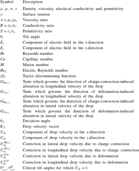
, respectively, cannot be neglected. Before presenting the mathematical model and the solution methodology, we provide a nomenclature for the important symbols in table 1.
Nomenclature for the important symbols used in the present analysis.

2.1 Governing equations and boundary conditions
Throughout our analysis, we present the governing equations and the respective boundary conditions in non-dimensional form unless specified otherwise. Under the consideration of the leaky dielectric model (Taylor Reference Taylor1966; Melcher & Taylor Reference Melcher and Taylor1969), the bulk fluids are charge-free and the electric potentials,
 ${\it\psi}_{i,e}$
, satisfy the Laplace equation of the form
 $$\begin{eqnarray}\left.\begin{array}{@{}l@{}}{\rm\nabla}^{2}{\it\psi}_{i}=0,\\ {\rm\nabla}^{2}{\it\psi}_{e}=0.\\ \end{array}\right\}\end{eqnarray}$$
The distribution of the electric potentials
 $({\it\psi}_{i,e})$
can be obtained by solving (2.1) by using the following boundary conditions (Saville Reference Saville1997; Xu & Homsy Reference Xu and Homsy2006):
-
(e1) specified unperturbed electric field at infinity; at
 $r\rightarrow \infty ,{\it\psi}_{e}\rightarrow {\it\psi}_{\infty }$
, where
$\boldsymbol{E}_{\infty }=-\boldsymbol{{\rm\nabla}}{\it\psi}_{\infty }$
and
$\boldsymbol{E}_{\infty }$
is the electric field vector applied at infinity;
-
(e2) bounded electric field inside the drop;
-
(e3) continuity of the electric potential at the drop interface; at
$r=r_{s},{\it\psi}_{i}={\it\psi}_{e}$
; -
(e4) charge conservation at the drop interface; at
$r=r_{s},\boldsymbol{n}\boldsymbol{\cdot }(R\boldsymbol{{\rm\nabla}}{\it\psi}_{i}-\boldsymbol{{\rm\nabla}}{\it\psi}_{e})=-Re_{E}\boldsymbol{{\rm\nabla}}_{s}\boldsymbol{\cdot }(q_{s}\boldsymbol{V}_{s})$
, where
$q_{s}=\boldsymbol{n}\boldsymbol{\cdot }(S\boldsymbol{{\rm\nabla}}{\it\psi}_{i}-\boldsymbol{{\rm\nabla}}{\it\psi}_{e})$
is the surface-charge distribution,
$\boldsymbol{n}$
represents the outward unit normal vector on the drop interface and
$\boldsymbol{V}_{s}$
is the fluid velocity at the drop interface; here
$\boldsymbol{{\rm\nabla}}_{s}=\boldsymbol{{\rm\nabla}}-\boldsymbol{n}(\boldsymbol{n}\boldsymbol{\cdot }\boldsymbol{{\rm\nabla}})$
is the surface gradient operator; the deformed drop interface is represented by the radial location
$r=r_{s}=1+f({\it\theta},{\it\phi})$
, where a non-zero
$f({\it\theta},{\it\phi})$
represents the deviation of the drop shape from sphericity; the normal unit vector
$\boldsymbol{n}$
can be defined as
$\boldsymbol{n}=\boldsymbol{{\rm\nabla}}(r-r_{s})/|\boldsymbol{{\rm\nabla}}(r-r_{s})|$
.












The velocity and pressure fields satisfy the Stokes equation and the condition of incompressibility of the form (Happel & Brenner Reference Happel and Brenner1981)
 $$\begin{eqnarray}\left.\begin{array}{@{}c@{}}\boldsymbol{{\rm\nabla}}p_{i}={\it\lambda}{\rm\nabla}^{2}\boldsymbol{u}_{i},\quad \boldsymbol{{\rm\nabla}}\boldsymbol{\cdot }\boldsymbol{u}_{i}=0,\\ \boldsymbol{{\rm\nabla}}p_{e}={\rm\nabla}^{2}\boldsymbol{u}_{e},\quad \boldsymbol{{\rm\nabla}}\boldsymbol{\cdot }\boldsymbol{u}_{e}=0,\end{array}\right\}\end{eqnarray}$$
where
 $\boldsymbol{u}_{i}$
and
 $p_{i}$
represent velocity and pressure fields inside the drop, respectively, while subscript
 $e$
has been used to denote the same quantities outside the drop. One thing to note here is that pressure
 $p_{i}$
and
 $p_{e}$
contain the contribution of the gravitational potential.
In a reference frame attached to the drop centre moving with a velocity
 $\boldsymbol{U}_{d}$
, the flow field satisfies the following boundary conditions:
-
(f1) uniform flow at infinity;
$\boldsymbol{u}_{e}(r\rightarrow \infty )=-\boldsymbol{U}_{d}$
; -
(f2) velocity and pressure fields inside the drop are bounded;
-
(f3) velocity fields satisfy the following boundary condition at the drop interface
$(r=r_{s})$
:
$\boldsymbol{u}_{i}=\boldsymbol{u}_{e}$
and
$\boldsymbol{u}_{i}\boldsymbol{\cdot }\boldsymbol{n}=\boldsymbol{u}_{e}\boldsymbol{\cdot }\boldsymbol{n}=0$
; -
(f4) stress balance at the drop interface
$(r=r_{s});{\bf\tau}_{e}\boldsymbol{\cdot }\boldsymbol{n}-{\bf\tau}_{i}\boldsymbol{\cdot }\boldsymbol{n}=(1/Ca)(\boldsymbol{{\rm\nabla}}\boldsymbol{\cdot }\boldsymbol{n})\boldsymbol{n}$
, where
${\bf\tau}_{i}$
and
${\bf\tau}_{e}$
represent the total stress tensors consisting of the hydrodynamic and electrical effects of the internal and external fluid, respectively.







2.2 Expansion in perturbation of
$Re_{E}$
and
$Ca$


The above equations and boundary conditions represent a two-way coupled electrohydrodynamic problem where electric field affects the flow field via the generation of Maxwell stress at the drop interface, while the flow field affects the electric field by redistributing the surface charges by convection (Xu & Homsy Reference Xu and Homsy2006; He, Salipante & Vlahovska Reference He, Salipante and Vlahovska2013; Lanauze et al.
Reference Lanauze, Walker and Khair2015). On top of that, the drop interface deforms and the drop shape function is a priori unknown. For problems dealing with drop motion and deformation, it is typical to perform a regular domain perturbation in orders of capillary number. But here we also would like to consider the fluid-flow-induced redistribution of surface charges and subsequent alteration in drop velocity. Towards this, we go ahead to solve the problem under consideration via a double asymptotic expansion in
 $Re_{E}$
and
 $Ca$
by assuming
 $$\begin{eqnarray}1\gg Re_{E},Ca\gg Re_{E}^{2},Re_{E}Ca,Ca^{2}.\end{eqnarray}$$
Now, we expand the electric potential, velocity, pressure, stress fields and the unknown drop velocity in the following regular perturbation form
 $$\begin{eqnarray}\left.\begin{array}{@{}c@{}}\displaystyle {\it\psi}_{i,e}={\it\psi}_{i,e}^{(0)}+Re_{E}{\it\psi}_{i,e}^{(Re_{E})}+Ca\,{\it\psi}_{i,e}^{(Ca)}+\cdots \,,\\ \displaystyle \boldsymbol{u}_{i,e}=\boldsymbol{u}_{i,e}^{(0)}+Re_{E}\boldsymbol{u}_{i,e}^{(Re_{E})}+Ca\,\boldsymbol{u}_{i,e}^{(Ca)}+\cdots \,,\\ \displaystyle p_{i}=p_{i}^{(0)}+Re_{E}p_{i}^{(Re_{E})}+Ca\,p_{i}^{(Ca)}+\cdots \,,\\ \displaystyle p_{e}=\frac{1}{Ca}\,p_{e}^{(1/Ca)}+p_{e}^{(0)}+Re_{E}p_{e}^{(Re_{E})}+Ca\,p_{e}^{(Ca)}+\cdots \,,\\ \displaystyle {\bf\tau}_{i}={\bf\tau}_{i}^{(0)}+Re_{E}{\bf\tau}_{i}^{(Re_{E})}+Ca\,{\bf\tau}_{i}^{(Ca)}+\cdots \,,\\ \displaystyle {\bf\tau}_{e}=\frac{1}{Ca}{\bf\tau}_{e}^{(1/Ca)}+{\bf\tau}_{e}^{(0)}+Re_{E}{\bf\tau}_{e}^{(Re_{E})}+Ca\,{\bf\tau}_{e}^{(Ca)}+\cdots \,,\\ \displaystyle \boldsymbol{U}_{d}=\boldsymbol{U}_{d}^{(0)}+Re_{E}\boldsymbol{U}_{d}^{(Re_{E})}+Ca\,\boldsymbol{U}_{d}^{(Ca)}+\cdots \,.\end{array}\right\}\end{eqnarray}$$
Here
 $\boldsymbol{U}_{d}^{(0)}$
is the drop velocity in the absence of interfacial charge convection and shape deformation,
 $\boldsymbol{U}_{d}^{(Re_{E})}$
denotes the first contribution of charge convection on the drop velocity and
 $\boldsymbol{U}_{d}^{(Ca)}$
is the first contribution of shape deformation on the drop velocity. One thing to note here is that we have included
 $p_{e}^{(1/Ca)}$
and
 ${\bf\tau}_{e}^{(1/Ca)}$
to balance the Laplace pressure across the drop interface (Leal Reference Leal2007).
The deformed shape of the drop is also expanded in the following form
 $$\begin{eqnarray}r_{s}=1+f=1+Ca\,f^{(Ca)}+Ca\,Re_{E}f^{(Ca\,Re_{E})}+Ca^{2}f^{(Ca^{2})}+\cdots \,,\end{eqnarray}$$
where
 $f^{(Ca)}$
,
 $f^{(Ca\,Re_{E})}$
and
 $f^{(Ca^{2})}$
are the corrections to the deformed drop shape at different orders of approximation and each are
 $O(1)$
quantity. An important thing to note is that the first effect of charge convection on the drop shape appears at
 $O(Ca\,Re_{E})$
. The outward unit normal
 $\boldsymbol{n}$
and the curvature of the deformed drop shape,
 $\boldsymbol{{\rm\nabla}}\boldsymbol{\cdot }\boldsymbol{n}$
, can be calculated using (2.5) as (Wohl & Rubinow Reference Wohl and Rubinow1974; Ajayi Reference Ajayi1978; Chan & Leal Reference Chan and Leal1979)
 $$\begin{eqnarray}\displaystyle \boldsymbol{n}=\frac{\boldsymbol{{\rm\nabla}}(r-f)}{|\boldsymbol{{\rm\nabla}}(r-f)|} & = & \displaystyle \left[\boldsymbol{e}_{r}-Ca\boldsymbol{{\rm\nabla}}f^{(Ca)}-Ca\,Re_{E}\boldsymbol{{\rm\nabla}}f^{(Ca\,Re_{E})}\vphantom{\left[\boldsymbol{{\rm\nabla}}f^{(Ca^{2})}+{\displaystyle \frac{1}{2}}(\boldsymbol{{\rm\nabla}}f^{(Ca)}\boldsymbol{\cdot }\boldsymbol{{\rm\nabla}}f^{(Ca)})\boldsymbol{e}_{r}\right]}\right.\nonumber\\ \displaystyle & & \displaystyle \left.-\,Ca^{2}\left[\boldsymbol{{\rm\nabla}}f^{(Ca^{2})}+\frac{1}{2}(\boldsymbol{{\rm\nabla}}f^{(Ca)}\boldsymbol{\cdot }\boldsymbol{{\rm\nabla}}f^{(Ca)})\boldsymbol{e}_{r}\right]-\cdots \,\right],\end{eqnarray}$$
and
 $$\begin{eqnarray}\displaystyle \boldsymbol{{\rm\nabla}}\boldsymbol{\cdot }\boldsymbol{n} & = & \displaystyle [2-Ca(2f^{(Ca)}+{\rm\nabla}^{2}f^{(Ca)})-Ca\,Re_{E}(2f^{(Ca\,Re_{E})}+{\rm\nabla}^{2}f^{(Ca\,Re_{E})})\nonumber\\ \displaystyle & & \displaystyle -\,Ca^{2}\{-2f^{(Ca)}(f^{(Ca)}+{\rm\nabla}^{2}f^{(Ca)})+2f^{(Ca^{2})}+{\rm\nabla}^{2}f^{(Ca^{2})}\}-\cdots ].\end{eqnarray}$$
Considering the above, the governing equations for the electric potentials
 $({\it\psi}_{i,e}^{(0)})$
at the leading order are given as
 $$\begin{eqnarray}\left.\begin{array}{@{}c@{}}{\rm\nabla}^{2}{\it\psi}_{i}^{(0)}=0,\\ {\rm\nabla}^{2}{\it\psi}_{e}^{(0)}=0,\\ \end{array}\right\}\end{eqnarray}$$
which are subjected to the following boundary conditions
 $$\begin{eqnarray}\displaystyle \left.\begin{array}{@{}c@{}}{\it\psi}_{e}^{(0)}|_{r\rightarrow \infty }\rightarrow {\it\psi}_{\infty },\\ {\it\psi}_{i}^{(0)}\text{ bounded for }r<1,\\ {\it\psi}_{e}^{(0)}|_{r=1}={\it\psi}_{i}^{(0)}|_{r=1},\\ \boldsymbol{e}_{r}\boldsymbol{\cdot }(R\boldsymbol{{\rm\nabla}}{\it\psi}_{i}^{(0)}-\boldsymbol{{\rm\nabla}}{\it\psi}_{e}^{(0)})|_{r=1}=0,\end{array}\right\} & & \displaystyle\end{eqnarray}$$
where
 ${\it\xi}|_{r=1}$
represents the evaluation of the quantity
 ${\it\xi}$
at the spherical drop interface
 $(r=1)$
.
The leading-order velocity and pressure fields
 $(\boldsymbol{u}_{i,e}^{(0)},p_{i,e}^{(0)})$
satisfy the following governing equations
 $$\begin{eqnarray}\left.\begin{array}{@{}c@{}}\boldsymbol{{\rm\nabla}}p_{i}^{(0)}={\it\lambda}{\rm\nabla}^{2}\boldsymbol{u}_{i}^{(0)},\quad \boldsymbol{{\rm\nabla}}\boldsymbol{\cdot }\boldsymbol{u}_{i}^{(0)}=0,\\ \boldsymbol{{\rm\nabla}}p_{e}^{(0)}={\rm\nabla}^{2}\boldsymbol{u}_{e}^{(0)},\quad \boldsymbol{{\rm\nabla}}\boldsymbol{\cdot }\boldsymbol{u}_{e}^{(0)}=0,\end{array}\right\}\end{eqnarray}$$
which are subjected to the following boundary conditions
 $$\begin{eqnarray}\left.\begin{array}{@{}c@{}}\boldsymbol{u}_{e}^{(0)}|_{r\rightarrow \infty }\rightarrow (-\boldsymbol{U}_{d}^{(0)}),\\ \boldsymbol{u}_{i}^{(0)}\text{ is bounded for }r<1,\\ \boldsymbol{u}_{e}^{(0)}|_{r=1}=\boldsymbol{u}_{i}^{(0)}|_{r=1},\\ \boldsymbol{u}_{e}^{(0)}|_{r=1}\boldsymbol{\cdot }\boldsymbol{e}_{r}=\boldsymbol{u}_{i}^{(0)}|_{r=1}\boldsymbol{\cdot }\boldsymbol{e}_{r}=0,\\ \boldsymbol{e}_{r}\boldsymbol{\cdot }({\bf\tau}_{e}^{(0)}-{\bf\tau}_{i}^{(0)})|_{r=1}\boldsymbol{\cdot }(\boldsymbol{I}-\boldsymbol{e}_{r}\boldsymbol{e}_{r})=0,\\ \boldsymbol{e}_{r}\boldsymbol{\cdot }({\bf\tau}_{e}^{(0)}-{\bf\tau}_{i}^{(0)})|_{r=1}\boldsymbol{\cdot }\boldsymbol{e}_{r}=-(2f^{(Ca)}+{\rm\nabla}^{2}f^{(Ca)}).\\ \end{array}\right\}\end{eqnarray}$$
One thing to note here is that the constant term present in the expression for the curvature (2.7) does not appear in the normal stress balance (last boundary condition of (2.11)) because of the fact that the
 $2/Ca$
term is balanced by
 $(1/Ca)p_{e}^{(1/Ca)}$
.
On similar lines, we obtain the following governing equations for the
 $O(Re_{E})$
electric potentials
 $({\it\psi}_{i,e}^{(Re_{E})})$
 $$\begin{eqnarray}\left.\begin{array}{@{}c@{}}{\rm\nabla}^{2}{\it\psi}_{i}^{(Re_{E})}=0,\\ {\rm\nabla}^{2}{\it\psi}_{e}^{(Re_{E})}=0,\\ \end{array}\right\}\end{eqnarray}$$
which are subjected to the, now altered,
 $O(Re_{E})$
boundary conditions (Feng Reference Feng1999; Xu & Homsy Reference Xu and Homsy2006)
 $$\begin{eqnarray}\left.\begin{array}{@{}c@{}}{\it\psi}_{e}^{(Re_{E})}|_{r\rightarrow \infty }\rightarrow 0,\\ {\it\psi}_{i}^{(Re_{E})}\text{ bounded for }r<1,\\ {\it\psi}_{i}^{(Re_{E})}|_{r=1}={\it\psi}_{e}^{(Re_{E})}|_{r=1},\\ \boldsymbol{e}_{r}\boldsymbol{\cdot }(R\boldsymbol{{\rm\nabla}}{\it\psi}_{i}^{(Re_{E})}-\boldsymbol{{\rm\nabla}}{\it\psi}_{e}^{(Re_{E})})|_{r=1}=-\boldsymbol{{\rm\nabla}}_{s}\boldsymbol{\cdot }(q_{s}^{(0)}\boldsymbol{V}_{s}^{(0)})|_{r=1},\\ \quad \text{where }q_{s}^{(0)}=\boldsymbol{e}_{r}\boldsymbol{\cdot }(S\boldsymbol{{\rm\nabla}}{\it\psi}_{i}^{(0)}-\boldsymbol{{\rm\nabla}}{\it\psi}_{e}^{(0)})|_{r=1}.\\ \end{array}\right\}\end{eqnarray}$$
It is to be noted that in the boundary condition for the normal electric field, the effect of surface-charge convection now appears through the redistribution of the surface charge.
The
 $O(Re_{E})$
velocity and pressure fields
 $(\boldsymbol{u}_{i,e}^{(Re_{E})},p_{i,e}^{(Re_{E})})$
satisfy the following governing equations
 $$\begin{eqnarray}\left.\begin{array}{@{}c@{}}\boldsymbol{{\rm\nabla}}p_{i}^{(Re_{E})}={\it\lambda}{\rm\nabla}^{2}\boldsymbol{u}_{i}^{(Re_{E})},\quad \boldsymbol{{\rm\nabla}}\boldsymbol{\cdot }\boldsymbol{u}_{i}^{(Re_{E})}=0,\\ \boldsymbol{{\rm\nabla}}p_{e}^{(Re_{E})}={\rm\nabla}^{2}\boldsymbol{u}_{e}^{(Re_{E})},\quad \boldsymbol{{\rm\nabla}}\boldsymbol{\cdot }\boldsymbol{u}_{e}^{(Re_{E})}=0,\\ \end{array}\right\}\end{eqnarray}$$
which are subjected to the boundary conditions
 $$\begin{eqnarray}\left.\begin{array}{@{}c@{}}\boldsymbol{u}_{e}^{(Re_{E})}|_{r\rightarrow \infty }\rightarrow (-\boldsymbol{U}_{d}^{(Re_{E})}),\\ \boldsymbol{u}_{i}^{(Re_{E})}\text{ is bounded for }r<1,\\ \boldsymbol{u}_{e}^{(Re_{E})}|_{r=1}=\boldsymbol{u}_{i}^{(Re_{E})}|_{r=1},\\ \boldsymbol{u}_{e}^{(Re_{E})}|_{r=1}\boldsymbol{\cdot }\boldsymbol{e}_{r}=\boldsymbol{u}_{i}^{(Re_{E})}|_{r=1}\boldsymbol{\cdot }\boldsymbol{e}_{r}=0,\\ \boldsymbol{e}_{r}\boldsymbol{\cdot }({\bf\tau}_{e}^{(Re_{E})}-{\bf\tau}_{i}^{(Re_{E})})|_{r=1}\boldsymbol{\cdot }(\boldsymbol{I}-\boldsymbol{e}_{r}\boldsymbol{e}_{r})=0,\\ \boldsymbol{e}_{r}\boldsymbol{\cdot }({\bf\tau}_{e}^{(Re_{E})}-{\bf\tau}_{i}^{(Re_{E})})|_{r=1}\boldsymbol{\cdot }\boldsymbol{e}_{r}=-(2f^{(Ca\,Re_{E})}+{\rm\nabla}^{2}f^{(Ca\,Re_{E})}).\end{array}\right\}\end{eqnarray}$$
The governing equations for the electric potentials
 $({\it\psi}_{i,e}^{(Ca)})$
at the
 $O(Ca)$
are given by
 $$\begin{eqnarray}\left.\begin{array}{@{}c@{}}{\rm\nabla}^{2}{\it\psi}_{i}^{(Ca)}=0,\\ {\rm\nabla}^{2}{\it\psi}_{e}^{(Ca)}=0,\end{array}\right\}\end{eqnarray}$$
which are subjected to the, now altered,
 $O(Ca)$
boundary conditions (Feng Reference Feng1999; Xu & Homsy Reference Xu and Homsy2006)
 $$\begin{eqnarray}\left.\begin{array}{@{}c@{}}{\it\psi}_{e}^{(Ca)}|_{r\rightarrow \infty }\rightarrow 0,\\ {\it\psi}_{i}^{(Ca)}\text{ bounded for }r<1,\\ \left[{\it\psi}_{e}|_{r=1+Ca\,f^{(Ca)}}\right]^{(Ca)}=\left[{\it\psi}_{i}|_{r=1+Ca\,f^{(Ca)}}\right]^{(Ca)},\\ \left[\boldsymbol{n}\boldsymbol{\cdot }(R\boldsymbol{{\rm\nabla}}{\it\psi}_{i}-\boldsymbol{{\rm\nabla}}{\it\psi}_{e})|_{r=1+Ca\,f^{(Ca)}}\right]^{(Ca)}=0,\\ \end{array}\right\}\end{eqnarray}$$
where
 $[{\it\xi}|_{r=1+Ca\,f^{(Ca)}}]^{(Ca)}$
represents the
 $O(Ca)$
contribution from the quantity
 ${\it\xi}$
evaluated at the deformed drop interface
 $r=1+Ca\,f^{(Ca)}$
. The
 $O(Ca)$
contributions can be obtained by performing the Taylor series expansion about
 $r=1$
and collecting the terms which are
 $O(Ca)$
, in the following way
 $$\begin{eqnarray}\displaystyle \left.\begin{array}{@{}l@{}}\displaystyle {\it\xi}|_{r=1+Ca\,f^{(Ca)}}={\it\xi}^{(0)}|_{r=1}\!+Re_{E}{\it\xi}^{(Re_{E})}|_{r=1}+Ca\left(\!{\it\xi}^{(Ca)}|_{r=1}\!+f^{(Ca)}\frac{\partial {\it\xi}^{(0)}}{\partial r}\bigg|_{r=1}\right)\!+\cdots \,,\!\\ \Rightarrow \displaystyle \left[\left.{\it\xi}\right|_{r=1+Ca\,f^{(Ca)}}\right]^{(Ca)}=\left({\it\xi}^{(Ca)}|_{r=1}+f^{(Ca)}\frac{\partial {\it\xi}^{(0)}}{\partial r}\bigg|_{r=1}\right).\end{array}\right\}\qquad & & \displaystyle \nonumber\\ \displaystyle & & \displaystyle\end{eqnarray}$$
The
 $O(Ca)$
velocity and pressure fields
 $(\boldsymbol{u}_{i,e}^{(Ca)},p_{i,e}^{(Ca)})$
satisfy the following governing equations
 $$\begin{eqnarray}\left.\begin{array}{@{}c@{}}\boldsymbol{{\rm\nabla}}p_{i}^{(Ca)}={\it\lambda}{\rm\nabla}^{2}\boldsymbol{u}_{i}^{(Ca)},\quad \boldsymbol{{\rm\nabla}}\boldsymbol{\cdot }\boldsymbol{u}_{i}^{(Ca)}=0,\\ \boldsymbol{{\rm\nabla}}p_{e}^{(Ca)}={\rm\nabla}^{2}\boldsymbol{u}_{e}^{(Ca)},\quad \boldsymbol{{\rm\nabla}}\boldsymbol{\cdot }\boldsymbol{u}_{e}^{(Ca)}=0,\end{array}\right\}\end{eqnarray}$$
which are subjected to the following boundary conditions
 $$\begin{eqnarray}\displaystyle \left.\begin{array}{@{}c@{}}\left.\boldsymbol{u}_{e}^{(Ca)}\right|_{r\rightarrow \infty }\rightarrow (-\boldsymbol{U}_{d}^{(Ca)}),\\ \boldsymbol{u}_{i}^{(Ca)}\text{ is bounded for }r<1,\\ \left[\left.\boldsymbol{u}_{e}\right|_{r=1+Ca\,f^{(Ca)}}\right]^{(Ca)}=\left[\left.\boldsymbol{u}_{i}\right|_{r=1+Ca\,f^{(Ca)}}\right]^{(Ca)},\\ \left[\left.\boldsymbol{u}_{e}\right|_{r=1+Ca\,f^{(Ca)}}\boldsymbol{\cdot }\boldsymbol{n}\right]^{(Ca)}=\left[\left.\boldsymbol{u}_{i}\right|_{r=1+Ca\,f^{(Ca)}}\boldsymbol{\cdot }\boldsymbol{n}\right]^{(Ca)}=0,\\ \left[\boldsymbol{n}\boldsymbol{\cdot }\left.\left({\bf\tau}_{e}-{\bf\tau}_{i}\right)\right|_{r=1+Ca\,f^{(Ca)}}\boldsymbol{\cdot }\left(\boldsymbol{I}-\boldsymbol{n}\boldsymbol{n}\right)\right]^{(Ca)}=0,\\ \left[\boldsymbol{n}\boldsymbol{\cdot }\left({\bf\tau}_{e}-{\bf\tau}_{i}\right)|_{r=1+Ca\,f^{(Ca)}}\boldsymbol{\cdot }\boldsymbol{n}\right]^{(Ca)}=2f^{(Ca)}\left(f^{(Ca)}+{\rm\nabla}^{2}f^{(Ca)}\right)-(2f^{(Ca^{2})}+{\rm\nabla}^{2}f^{(Ca^{2})}).\end{array}\right\} & & \displaystyle \nonumber\\ \displaystyle & & \displaystyle\end{eqnarray}$$
3 Asymptotic solution for small charge convection and small shape deformation
3.1 Description of electric potential and flow fields
At each order of perturbation, the electric potentials
 $({\it\psi}_{i,e}^{(k)})$
satisfy the Laplace equation, solution of which is given by
 $$\begin{eqnarray}\left.\begin{array}{@{}c@{}}\displaystyle {\it\psi}_{i}^{(k)}=\mathop{\sum }_{n=0}^{\infty }r^{n}[a_{n,m}^{(k)}\cos (m{\it\phi})+\hat{a}_{n,m}^{(k)}\sin (m{\it\phi})]P_{n,m}(\cos {\it\theta}),\\ \displaystyle {\it\psi}_{e}^{(k)}={\it\psi}_{\infty }^{(k)}+\mathop{\sum }_{n=0}^{\infty }r^{-n-1}[b_{-n-1,m}^{(k)}\cos (m{\it\phi})+\hat{b}_{-n-1,m}^{(k)}\sin (m{\it\phi})]P_{n,m}(\cos {\it\theta}),\end{array}\right\}\end{eqnarray}$$
where the superscript
 $k$
represents the order of perturbation. We only consider
 $k=0$
,
 $k=Re_{E}$
and
 $k=Ca$
. Here
 ${\it\psi}_{\infty }^{(k)}$
is the unperturbed applied potential at far field
 $(r\rightarrow \infty )$
having non-zero value only at the leading order of perturbation as
 ${\it\psi}_{\infty }^{(0)}=-r(E_{x}P_{1,1}\cos {\it\phi}+E_{z}P_{1,0})$
. Here
 $P_{n,m}(\cos {\it\theta})$
is the associated Legendre polynomial of degree
 $n$
and order
 $m$
with
 $\cos {\it\theta}$
as the argument. The unknown coefficients (
 $a_{n,m}^{(k)},\hat{a}_{n,m}^{(k)},b_{-n-1,m}^{(k)}$
and
 $\hat{b}_{-n-1,m}^{(k)}$
) can be determined at each order of perturbation by using respective boundary conditions.
As the velocity and pressure fields
 $(\boldsymbol{u}_{i,e}^{(k)},p_{i,e}^{(k)})$
satisfy the Stokes equation and the condition of incompressibility at each order of perturbation, we can represent the velocity and pressure fields inside the drop,
 $(\boldsymbol{u}_{i}^{(k)},p_{i}^{(k)})$
, by using the Lamb’s general solution in the following form (Happel & Brenner Reference Happel and Brenner1981)
 $$\begin{eqnarray}\displaystyle \boldsymbol{u}_{i}^{(k)} & = & \displaystyle \mathop{\sum }_{n=1}^{\infty }\left[\boldsymbol{{\rm\nabla}}\times \left(\boldsymbol{r}{\it\chi}_{n}^{(k)}\right)+\boldsymbol{{\rm\nabla}}{\it\Phi}_{n}^{(k)}\vphantom{\frac{n+3}{2\left(n+1\right)\left(2n+3\right){\it\lambda}}}\right.\nonumber\\ \displaystyle & & \displaystyle +\left.\frac{n+3}{2\left(n+1\right)\left(2n+3\right){\it\lambda}}r^{2}\boldsymbol{{\rm\nabla}}p_{n}^{(k)}-\frac{n}{\left(n+1\right)(2n+3){\it\lambda}}\boldsymbol{r}p_{n}^{(k)}\right],\end{eqnarray}$$
 $$\begin{eqnarray}p_{i}^{(k)}=\mathop{\sum }_{n=1}^{\infty }p_{n}^{(k)},\end{eqnarray}$$
whereas the velocity and pressure fields outside the drop,
 $(\boldsymbol{u}_{e}^{(k)},p_{e}^{(k)})$
, can be represented using Lamb’s general solution as (Happel & Brenner Reference Happel and Brenner1981)
 $$\begin{eqnarray}\displaystyle \boldsymbol{u}_{e}^{(k)} & \hspace{-2.0pt}=\hspace{-2.0pt} & \displaystyle -\boldsymbol{U}_{d}^{(k)}+\boldsymbol{v}_{e}^{(k)}\nonumber\\ \displaystyle & \hspace{-2.0pt}=\hspace{-2.0pt} & \displaystyle -\boldsymbol{U}_{d}^{(k)}+\mathop{\sum }_{n=1}^{\infty }\displaystyle \left[\boldsymbol{{\rm\nabla}}\times (\boldsymbol{r}{\it\chi}_{-n-1}^{(k)})+\boldsymbol{{\rm\nabla}}{\it\Phi}_{-n-1}^{(k)}\vphantom{\frac{n-2}{2n(2n-1)}}\right.\nonumber\\ \displaystyle \displaystyle & & \displaystyle \left.-\,\frac{n-2}{2n(2n-1)}r^{2}\boldsymbol{{\rm\nabla}}p_{-n-1}^{(k)}+\frac{n+1}{n(2n-1)}\boldsymbol{r}p_{-n-1}^{(k)}\right],\end{eqnarray}$$
 $$\begin{eqnarray}p_{e}^{(k)}=\mathop{\sum }_{n=1}^{\infty }p_{-n-1}^{\left(k\right)},\end{eqnarray}$$
where
 $\boldsymbol{v}_{e}^{(k)}$
is the disturbance velocity field outside the drop which vanishes at infinity. In (3.2) and (3.4),
 $\boldsymbol{r}$
represents the position vector of magnitude
 $r$
. The expressions of the solid harmonics present in the velocity and pressure fields (
 $p_{n}^{(k)},{\it\Phi}_{n}^{(k)},{\it\chi}_{n}^{(k)},p_{-n-1}^{(k)},{\it\Phi}_{-n-1}^{(k)}$
and
 ${\it\chi}_{-n-1}^{(k)}$
) are mentioned in appendix A.
3.2 Leading-order solution
At the leading order of perturbation, there is no charge convection, allowing the electric field to be decoupled from the flow field. Thus, the leading-order electric field distribution can be solved independently. The solution of (2.8) which gives the potential distribution inside and outside the drop can be easily obtained by linear combination of the potential distribution due to the component of electric field applied in the longitudinal direction
 $(E_{z})$
and potential distribution due to the component of electric field applied in the lateral direction
 $(E_{x})$
in the following form (Lee, Im & Kang Reference Lee, Im and Kang2000; Im & Kang Reference Im and Kang2003):
 $$\begin{eqnarray}\displaystyle {\it\psi}_{i}^{(0)} & \hspace{-2.0pt}=\hspace{-2.0pt} & \displaystyle {\it\psi}_{i,z}^{(0)}+{\it\psi}_{i,x}^{(0)}\nonumber\\ \displaystyle & \hspace{-2.0pt}=\hspace{-2.0pt} & \displaystyle -\left[\frac{3}{2+R}rP_{1,0}\right]E_{z}-\left[\frac{3\cos {\it\phi}}{2+R}rP_{1,1}\right]E_{x},\end{eqnarray}$$
 $$\begin{eqnarray}\displaystyle {\it\psi}_{e}^{(0)} & = & \displaystyle {\it\psi}_{e,z}^{(0)}+{\it\psi}_{e,x}^{(0)}\nonumber\\ \displaystyle & \hspace{-2.0pt}=\hspace{-2.0pt} & \displaystyle \left[-rP_{1,0}+\frac{(R-1)}{(2+R)}\frac{1}{r^{2}}P_{1,0}\right]E_{z}+\left[-rP_{1,1}\cos {\it\phi}+\frac{(R-1)\cos {\it\phi}}{(2+R)}\frac{1}{r^{2}}P_{1,1}\right]E_{x},\nonumber\\ \displaystyle & & \displaystyle\end{eqnarray}$$
where
 ${\it\psi}_{z}^{(0)}$
and
 ${\it\psi}_{x}^{(0)}$
represent the potential distributions due to
 $E_{z}$
and
 $E_{x}$
, respectively. The leading-order surface-charge distribution at the drop surface is also obtained by combining the charge distributions due to longitudinal and laterally applied electric fields in the following form (Lee et al.
Reference Lee, Im and Kang2000; Im & Kang Reference Im and Kang2003):
 $$\begin{eqnarray}\displaystyle q_{s}^{(0)} & = & \displaystyle q_{s,z}^{(0)}+q_{s,x}^{(0)}\nonumber\\ \displaystyle & = & \displaystyle \frac{3(R-S)}{R+2}[E_{z}P_{1,0}+E_{x}P_{1,1}\cos {\it\phi}].\end{eqnarray}$$
Calculation of the velocity and pressure fields can be easily done by using the linearity of the leading-order problem. The flow field generated due to
 $\boldsymbol{E}_{\infty }$
is called the Taylor solution
 $(\boldsymbol{u}^{E(0)},p^{E(0)})$
(Taylor Reference Taylor1966; Saville Reference Saville1997), and the flow field generated due to setting of the drop in gravitational field is the so-called Hadamard–Rybczynski solution
 $(\boldsymbol{u}^{g(0)},p^{g(0)})$
(Happel & Brenner Reference Happel and Brenner1981; Leal Reference Leal2007). These solutions are independent of each other. Hence, the leading-order solution is the linear combination of these two solutions. As the spherical harmonic representation is useful for further calculations, we represent the velocity and pressure fields in the following form (Lee et al.
Reference Lee, Im and Kang2000; Im & Kang Reference Im and Kang2003):
 $$\begin{eqnarray}\displaystyle \boldsymbol{u}_{i}^{(0)} & = & \displaystyle \boldsymbol{u}_{i}^{E(0)}+\boldsymbol{u}_{i}^{g(0)}\nonumber\\ \displaystyle & = & \displaystyle \left[\boldsymbol{{\rm\nabla}}\left({\it\Phi}_{1}^{(0)}+{\it\Phi}_{2}^{(0)}\right)+r^{2}\boldsymbol{{\rm\nabla}}\left(\frac{1}{5{\it\lambda}}p_{1}^{(0)}+\frac{5}{42{\it\lambda}}p_{2}^{(0)}\right)-\boldsymbol{r}\left(\frac{1}{10{\it\lambda}}p_{1}^{(0)}+\frac{2}{21{\it\lambda}}p_{2}^{(0)}\right)\right],\qquad\end{eqnarray}$$
 $$\begin{eqnarray}\displaystyle p_{i}^{(0)} & = & \displaystyle p^{E(0)}+p^{g(0)}\nonumber\\ \displaystyle & = & \displaystyle p_{1}^{(0)}+p_{2}^{(0)},\end{eqnarray}$$
 $$\begin{eqnarray}\displaystyle \boldsymbol{u}_{e}^{(0)} & \hspace{-2.0pt}=\hspace{-2.0pt} & \displaystyle \boldsymbol{u}_{e}^{E(0)}+\boldsymbol{u}_{e}^{g(0)}\nonumber\\ \displaystyle & \hspace{-2.0pt}=\hspace{-2.0pt} & \displaystyle \left[\boldsymbol{{\rm\nabla}}({\it\Phi}_{-2}^{(0)}+{\it\Phi}_{-3}^{(0)})+{\textstyle \frac{1}{2}}r^{2}\boldsymbol{{\rm\nabla}}p_{-2}^{(0)}+\boldsymbol{r}\left(2p_{-2}^{(0)}+{\textstyle \frac{1}{2}}p_{-3}^{(0)}\right)\right],\end{eqnarray}$$
 $$\begin{eqnarray}\displaystyle p_{e}^{(0)} & \hspace{-2.0pt}=\hspace{-2.0pt} & \displaystyle p_{e}^{E(0)}+p_{e}^{g(0)}\nonumber\\ \displaystyle & \hspace{-2.0pt}=\hspace{-2.0pt} & \displaystyle p_{-2}^{(0)}+p_{-3}^{(0)},\end{eqnarray}$$
where the complete expressions of the solid harmonics and their coefficients are given in appendix B.
The sedimenting velocity of a drop is obtained by imposing the force-free condition. At steady state, the buoyancy force balances the hydrodynamic force on the drop. In a dimensional form, this can be represented at the leading order as (Hetsroni & Haber Reference Hetsroni and Haber1970; Leal Reference Leal2007)
 $$\begin{eqnarray}\frac{4{\rm\pi}}{3}a^{3}({\it\rho}_{i}-{\it\rho}_{e})g\boldsymbol{e}_{z}-4{\rm\pi}\boldsymbol{{\rm\nabla}}\left(r^{3}\bar{p}_{-2}^{(0)}\right)=\mathbf{0},\end{eqnarray}$$
where
 $\bar{p}_{-2}^{(0)}$
is the dimensional solid harmonic. Using the previously prescribed non-dimensional scheme, equation (3.13) may be written as
 $$\begin{eqnarray}\left(\frac{3{\it\lambda}+2}{2{\it\lambda}+2}\right)\boldsymbol{e}_{z}-\boldsymbol{{\rm\nabla}}(r^{3}p_{-2}^{(0)})=\mathbf{0},\end{eqnarray}$$
where
 $\boldsymbol{e}_{z}=\cos {\it\theta}\boldsymbol{e}_{r}-\sin {\it\theta}\boldsymbol{e}_{{\it\theta}}$
and
 $p_{-2}^{(0)}=1/r^{2}[A_{-2,0}^{(0)}P_{1,0}+A_{-2,1}^{(0)}\cos {\it\phi}P_{1,1}+\hat{A}_{-2,1}^{(0)}\sin {\it\phi}P_{1,1}].$
The coefficients
 $A_{-2,0}^{(0)}$
,
 $A_{-2,1}^{(0)}$
and
 $\hat{A}_{-2,1}^{(0)}$
are given in appendix B. Now substituting the expression of
 $p_{-2}^{(0)}$
in (3.14), we obtain the drop velocity as
 $$\begin{eqnarray}U_{dx}^{(0)}=U_{dy}^{(0)}=0,\quad U_{dz}^{(0)}=1.\end{eqnarray}$$
This shows that at the leading order of perturbation the applied uniform electric field does not contribute to the force acting on the drop.
Towards determining the deformation of the drop, we decompose the correction term
 $f^{(Ca)}({\it\theta},{\it\phi})$
in the following surface harmonics form (Hetsroni & Haber Reference Hetsroni and Haber1970):
 $$\begin{eqnarray}f^{(Ca)}({\it\theta},{\it\phi})=\mathop{\sum }_{n=2}^{\infty }[L_{n,m}^{(Ca)}\cos (m{\it\phi})+\hat{L}_{n,m}^{(Ca)}\sin (m{\it\phi})]P_{n,m},\end{eqnarray}$$
where
 $L_{n,m}^{(Ca)}$
and
 $\hat{L}_{n,m}^{(Ca)}$
are the unknown coefficients. The non-zero coefficients
 $(L_{n,m}^{(Ca)},\hat{L}_{n,m}^{(Ca)})$
are obtained by satisfying the normal stress balance equation (last boundary condition of (2.11)) as
 $$\begin{eqnarray}L_{2,0}^{(Ca)}=\frac{3}{8}\frac{M(2E_{z}^{2}-E_{x}^{2}){\it\Omega}_{T}}{\left(R+2\right)^{2}},\quad L_{2,1}^{(Ca)}=\frac{3}{4}\frac{ME_{x}E_{z}{\it\Omega}_{T}}{(R+2)^{2}},\quad L_{2,2}^{\left(Ca\right)}=\frac{3}{16}\frac{ME_{x}^{2}{\it\Omega}_{T}}{\left(R+2\right)^{2}},\end{eqnarray}$$
where
 ${\it\Omega}_{T}=R^{2}+1-2S+(3/5)(R-S)((3{\it\lambda}+2)/({\it\lambda}+1))$
is the Taylor discriminating function (Saville Reference Saville1997; Vizika & Saville Reference Vizika and Saville2006).
3.3 The
$O(Re_{E})$
solution

Having obtained the leading-order velocity profile, we may now attempt to solve (2.12) and (2.14) which are subjected to the boundary conditions (2.13) and (2.15), respectively. The first effect of charge convection through the leading-order charge distribution and the velocity field is to affect the
 $O(Re_{E})$
electric field and, consequently, the
 $O(Re_{E})$
velocity and pressure fields. For convenience, we rewrite the boundary condition here:
 $\boldsymbol{e}_{r}\boldsymbol{\cdot }(R\boldsymbol{{\rm\nabla}}{\it\psi}_{i}^{(Re_{E})}-\boldsymbol{{\rm\nabla}}{\it\psi}_{e}^{(Re_{E})})|_{r=1}=-\boldsymbol{{\rm\nabla}}_{s}\boldsymbol{\cdot }(q_{s}^{(0)}\boldsymbol{V}_{s}^{(0)})|_{r=1}$
. This differs from the leading-order condition (i.e.
 $\boldsymbol{e}_{r}\boldsymbol{\cdot }(R\boldsymbol{{\rm\nabla}}{\it\psi}_{i}^{(0)}-\boldsymbol{{\rm\nabla}}{\it\psi}_{e}^{(0)})|_{r=1}=0$
). Given that the electric potential fields
 $({\it\psi}_{i,e}^{(Re_{E})})$
are harmonic functions, it is instructive to first evaluate the right-hand side of the charge convection boundary condition in order to establish the various surface harmonics that it may contain. It can be recast as (Kim & Karrila Reference Kim and Karrila1991)
 $$\begin{eqnarray}-\!\boldsymbol{{\rm\nabla}}_{s}\boldsymbol{\cdot }(q_{s}^{(0)}\boldsymbol{V}_{s}^{(0)})=-2(q_{s}^{(0)}\boldsymbol{V}_{s}^{(0)}\boldsymbol{\cdot }\boldsymbol{e}_{r})-\frac{1}{\sin {\it\theta}}\frac{\partial }{\partial {\it\theta}}(q_{s}^{(0)}\boldsymbol{V}_{s}^{(0)}\boldsymbol{\cdot }\boldsymbol{e}_{{\it\theta}})-\frac{1}{\sin {\it\theta}}\frac{\partial }{\partial {\it\phi}}(q_{s}^{(0)}\boldsymbol{V}_{s}^{(0)}\boldsymbol{\cdot }\boldsymbol{e}_{{\it\phi}}).\end{eqnarray}$$
By substituting the form of the velocity field (given in (3.9)) and the accumulated charge (from (3.8)) in terms of the leading-order electric field, we split the above expression into various surface harmonics by using the orthogonality of the spherical surface harmonics. If we write the expression given in (3.18) as
 $\sum _{n=0}^{\infty }\sum _{m=0}^{n}(Z_{n,m}\cos (m{\it\phi})+\hat{Z}_{n,m}\sin (m{\it\phi}))P_{n,m},$
we obtain the following non-zero terms:
 $Z_{1,0},Z_{1,1},Z_{2,0},Z_{2,1},Z_{3,0},Z_{3,1},Z_{3,2}$
and
 $Z_{3,3}$
. The complete expressions of the
 $Z$
values are given in appendix C. Thus, it is expected that
 $O(Re_{E})$
electric potential inside and outside the drop will have the following form:
 $$\begin{eqnarray}\displaystyle {\it\psi}_{i}^{(Re_{E})} & = & \displaystyle r[a_{1,0}^{\left(Re_{E}\right)}P_{1,0}+a_{1,1}^{(Re_{E})}P_{1,1}\cos {\it\phi}]+r^{2}[a_{2,0}^{(Re_{E})}P_{2,0}+a_{2,1}^{(Re_{E})}P_{2,1}\cos {\it\phi}]\nonumber\\ \displaystyle & & \displaystyle +\,r^{3}[a_{3,0}^{(Re_{E})}P_{3,0}+a_{3,1}^{(Re_{E})}P_{3,1}\cos {\it\phi}+a_{3,2}^{(Re_{E})}P_{3,2}\cos \left(2{\it\phi}\right)+a_{3,3}^{(Re_{E})}P_{3,3}\cos (3{\it\phi})],\nonumber\\ \displaystyle & & \displaystyle\end{eqnarray}$$
 $$\begin{eqnarray}\displaystyle {\it\psi}_{e}^{(Re_{E})} & = & \displaystyle \frac{1}{r^{2}}[b_{-2,0}^{(Re_{E})}P_{1,0}+b_{-2,1}^{(Re_{E})}P_{1,1}\cos {\it\phi}]+\frac{1}{r^{3}}[b_{-3,0}^{(Re_{E})}P_{2,0}+b_{-3,1}^{(Re_{E})}P_{2,1}\cos {\it\phi}]\nonumber\\ \displaystyle & & \displaystyle +\,\frac{1}{r^{4}}[b_{-4,0}^{(Re_{E})}P_{3,0}+b_{-4,1}^{(Re_{E})}P_{3,1}\cos {\it\phi}+b_{-4,2}^{(Re_{E})}P_{3,2}\cos (2{\it\phi})+b_{-4,3}^{(Re_{E})}P_{3,3}\cos (3{\it\phi})].\nonumber\\ \displaystyle & & \displaystyle\end{eqnarray}$$
Now, we use the rest of the boundary conditions from (2.13) and obtain the above unknown coefficients
 $(a_{n,m}^{(Re_{E})}\,\;\text{and}\;\,b_{-n-1,m}^{(Re_{E})})$
which are given in appendix D. Surface-charge distribution at this order is obtained as
 $$\begin{eqnarray}\displaystyle q_{s}^{(Re_{E})} & = & \displaystyle \boldsymbol{e}_{r}\boldsymbol{\cdot }(S\boldsymbol{{\rm\nabla}}{\it\psi}_{i}^{(Re_{E})}-\boldsymbol{{\rm\nabla}}{\it\psi}_{e}^{(Re_{E})})\nonumber\\ \displaystyle & = & \displaystyle \displaystyle \left[\left(\frac{2+S}{2+R}\right)\left[Z_{1,0}P_{1,0}+Z_{1,1}P_{1,1}\cos {\it\phi}\right]\right.\nonumber\\ \displaystyle & & \displaystyle \displaystyle +\,\left(\frac{3+2S}{3+2R}\right)[Z_{2,0}P_{2,0}+Z_{2,1}P_{2,1}\cos {\it\phi}]\nonumber\\ \displaystyle & & \displaystyle +\displaystyle \left(\frac{4+3S}{4+3R}\right)\left[Z_{3,0}P_{3,0}+Z_{3,1}P_{3,1}\cos {\it\phi}\right.\nonumber\\ \displaystyle & & \displaystyle +\,\!\left.\vphantom{\left({\displaystyle \frac{2+S}{2+R}}\right)}\left.Z_{3,2}P_{3,2}\cos (2{\it\phi})+Z_{3,3}P_{3,3}\cos (3{\it\phi})\right]\right].\end{eqnarray}$$
The
 $O(Re_{E})$
velocity and pressure fields inside and outside the drop are obtained in the following form:
 $$\begin{eqnarray}\displaystyle \displaystyle \boldsymbol{u}_{i}^{(Re_{E})} & = & \displaystyle \mathop{\sum }_{n=1}^{4}\left[\boldsymbol{{\rm\nabla}}\times \left(\boldsymbol{r}{\it\chi}_{n}^{\left(Re_{E}\right)}\right)+\boldsymbol{{\rm\nabla}}{\it\Phi}_{n}^{(Re_{E})}+\frac{n+3}{2\left(n+1\right)\left(2n+3\right){\it\lambda}}r^{2}\boldsymbol{{\rm\nabla}}p_{n}^{(Re_{E})}\right.\nonumber\\ \displaystyle & & \displaystyle \left.-\,\frac{n}{\left(n+1\right)\left(2n+3\right){\it\lambda}}\boldsymbol{r}p_{n}^{(Re_{E})}\right],\end{eqnarray}$$
 $$\begin{eqnarray}\displaystyle \displaystyle p_{i}^{(Re_{E})}=\mathop{\sum }_{n=1}^{4}p_{n}^{\left(Re_{E}\right)}, & & \displaystyle\end{eqnarray}$$
 $$\begin{eqnarray}\displaystyle \displaystyle \boldsymbol{u}_{e}^{(Re_{E})} & = & \displaystyle \mathop{\sum }_{n=1}^{4}\displaystyle \left[\boldsymbol{{\rm\nabla}}\times (\boldsymbol{r}{\it\chi}_{-n-1}^{(Re_{E})})+\boldsymbol{{\rm\nabla}}{\it\Phi}_{-n-1}^{(Re_{E})}-\frac{n-2}{2n(2n-1)}r^{2}\boldsymbol{{\rm\nabla}}p_{-n-1}^{(Re_{E})}\right.\nonumber\\ \displaystyle & & \displaystyle \displaystyle \left.+\,\frac{n+1}{n(2n-1)}\boldsymbol{r}p_{-n-1}^{(Re_{E})}\right],\end{eqnarray}$$
 $$\begin{eqnarray}\displaystyle & \displaystyle p_{e}^{(Re_{E})}=\mathop{\sum }_{n=1}^{4}p_{-n-1}^{(Re_{E})}. & \displaystyle\end{eqnarray}$$
One thing to note here is that the flow field contains non-zero harmonics up to
 $n=4$
. The solid harmonics present in (3.22)–(3.25) are obtained by application of the boundary conditions (2.15). We do not present those here for the sake of brevity. However, the detailed procedure to obtain these unknown solid harmonics is given in the supplementary material available at http://dx.doi.org/10.1017/jfm.2016.84. To determine the drop velocity, we need the expression of
 $p_{-2}^{(Re_{E})}$
which is given by
 $$\begin{eqnarray}p_{-2}^{(Re_{E})}=\frac{1}{r^{2}}[A_{-2,0}^{(Re_{E})}P_{1,0}+A_{-2,1}^{(Re_{E})}\cos {\it\phi}P_{1,1}+\hat{A}_{-2,1}^{(Re_{E})}\sin {\it\phi}P_{1,1}],\end{eqnarray}$$
where
 $A_{-2,0}^{(Re_{E})}$
,
 $A_{-2,1}^{(Re_{E})}$
and
 $\hat{A}_{-2,1}^{(Re_{E})}$
are obtained as
 $$\begin{eqnarray}\left.\begin{array}{@{}l@{}}\displaystyle A_{-2,0}^{(Re_{E})}=\left(\frac{3{\it\lambda}+2}{2{\it\lambda}+2}\right)U_{dz}^{(Re_{E})}+\frac{3M(3R-S+3)(R-S)\left(4E_{z}^{2}+3E_{x}^{2}\right)}{20({\it\lambda}+1)^{2}(2+R)^{2}\left(3+2R\right)},\\ \displaystyle A_{-2,1}^{(Re_{E})}=\left(\frac{3{\it\lambda}+2}{2{\it\lambda}+2}\right)U_{dx}^{(Re_{E})}+\frac{3M(3R-S+3)(R-S)E_{x}E_{z}}{20({\it\lambda}+1)^{2}(2+R)^{2}(3+2R)},\\ \displaystyle \hat{A}_{-2,1}^{(Re_{E})}=\left(\frac{3{\it\lambda}+2}{2{\it\lambda}+2}\right)U_{dy}^{(Re_{E})}.\end{array}\right\}\end{eqnarray}$$
In tune with the leading-order drop velocity estimation, we may proceed in a similar fashion to evaluate
 $O(Re_{E})$
drop velocity
 $$\begin{eqnarray}\boldsymbol{{\rm\nabla}}(r^{3}p_{-2}^{(Re_{E})})=\mathbf{0}.\end{eqnarray}$$
Thus, employing the force-free condition at
 $O(Re_{E})$
, we obtain drop velocity at
 $O(Re_{E})$
as
 $$\begin{eqnarray}\left.\begin{array}{@{}l@{}}\displaystyle U_{dx}^{(Re_{E})}=\frac{3}{10}\frac{M(S-R)(3R-S+3)E_{x}E_{z}}{(3+2R)(R+2)^{2}(2+3{\it\lambda})({\it\lambda}+1)},\\ \displaystyle U_{dy}^{(Re_{E})}=0,\\ \displaystyle U_{dz}^{(Re_{E})}=\frac{3}{10}\frac{M(S-R)(3R-S+3)\left(4E_{z}^{2}+3E_{x}^{2}\right)}{\left(3+2R\right)(R+2)^{2}(2+3{\it\lambda})({\it\lambda}+1)}.\end{array}\right\}\end{eqnarray}$$
3.4 The
$O(Ca)$
solution

On similar lines, the electric potentials at
 $O(Ca)$
are obtained as
 $$\begin{eqnarray}\displaystyle {\it\psi}_{i}^{(Ca)} & = & \displaystyle r[a_{1,0}^{(Ca)}P_{1,0}+a_{1,1}^{(Ca)}P_{1,1}\cos {\it\phi}]+r^{3} [a_{3,0}^{(Ca)}P_{3,0}+a_{3,1}^{(Ca)}P_{3,1}\cos {\it\phi}\nonumber\\ \displaystyle & & \displaystyle +\,a_{3,2}^{(Ca)}P_{3,2}\cos \left(2{\it\phi}\right)+a_{3,3}^{(Ca)}P_{3,3}\cos (3{\it\phi})],\end{eqnarray}$$
 $$\begin{eqnarray}\displaystyle {\it\psi}_{e}^{(Ca)} & = & \displaystyle \frac{1}{r^{2}}[b_{-2,0}^{(Ca)}P_{1,0}+b_{-2,1}^{(Ca)}P_{1,1}\cos {\it\phi}]+\frac{1}{r^{4}} [b_{-4,0}^{(Ca)}P_{3,0}+b_{-4,1}^{(Ca)}P_{3,1}\cos {\it\phi}\nonumber\\ \displaystyle & & \displaystyle +\,b_{-4,2}^{(Ca)}P_{3,2}\cos (2{\it\phi})+b_{-4,3}^{(Ca)}P_{3,3}\cos (3{\it\phi})],\end{eqnarray}$$
where the detailed expressions of the coefficients (
 $a_{n,m}^{(Ca)}$
and
 $b_{-n-1,m}^{(Ca)}$
) are given in appendix E.
The velocity and pressure fields at
 $O(Ca)$
are obtained in a similar form as given in (3.22)–(3.25). In this case also the flow field contains non-zero harmonics up to
 $n=4$
. The solid harmonics are obtained by application of the boundary conditions (2.20). We do not present those here for the sake of brevity. However, the detailed procedure to obtain these unknown solid harmonics is given in the supplementary material. The solid harmonic
 $p_{-2}^{(Ca)}$
, necessary to proceed further to calculate the drop velocity, is given by
 $$\begin{eqnarray}p_{-2}^{(Ca)}=\frac{1}{r^{2}}[A_{-2,0}^{(Ca)}P_{1,0}+A_{-2,1}^{(Ca)}\cos {\it\phi}P_{1,1}+\hat{A}_{-2,1}^{(Ca)}\sin {\it\phi}P_{1,1}],\end{eqnarray}$$
where
 $A_{-2,0}^{(Ca)}$
,
 $A_{-2,1}^{(Ca)}$
and
 $\hat{A}_{-2,1}^{(Ca)}$
are obtained as
 $$\begin{eqnarray}\left.\begin{array}{@{}l@{}}\displaystyle A_{-2,0}^{(Ca)}=\left(\frac{3{\it\lambda}+2}{2{\it\lambda}+2}\right)U_{dz}^{(Ca)}-\frac{1}{10}\left(\frac{3{\it\lambda}^{2}-{\it\lambda}+8}{\left({\it\lambda}+1\right)^{2}}\right)L_{2,0}^{(Ca)},\\ \displaystyle A_{-2,1}^{(Ca)}=\left(\frac{3{\it\lambda}+2}{2{\it\lambda}+2}\right)U_{dx}^{(Ca)}-\frac{3}{20}\left(\frac{3{\it\lambda}^{2}-{\it\lambda}+8}{\left({\it\lambda}+1\right)^{2}}\right)L_{2,1}^{(Ca)},\\ \displaystyle \hat{A}_{-2,1}^{(Ca)}=\left(\frac{3{\it\lambda}+2}{2{\it\lambda}+2}\right)U_{dy}^{(Ca)}.\end{array}\right\}\end{eqnarray}$$
Now, the force-free condition at
 $O(Ca)$
is given by
 $$\begin{eqnarray}\boldsymbol{{\rm\nabla}}(r^{3}p_{-2}^{(Ca)})=\mathbf{0},\end{eqnarray}$$
which yields the following form of the drop velocity
 $$\begin{eqnarray}\left.\begin{array}{@{}l@{}}\displaystyle U_{dx}^{(Ca)}=\frac{9}{40}\frac{M\!\left(3{\it\lambda}^{2}-{\it\lambda}+8\right)E_{x}E_{z}{\it\Omega}_{T}}{\left(R+2\right)^{2}\left(2+3{\it\lambda}\right)\left({\it\lambda}+1\right)},\\ U_{dy}^{(Ca)}=0,\\ \displaystyle U_{dz}^{(Ca)}=\frac{3}{40}\frac{M\!\left(3{\it\lambda}^{2}-{\it\lambda}+8\right)\left(2E_{z}^{2}-E_{x}^{2}\right){\it\Omega}_{T}}{(R+2)^{2}\left(2+3{\it\lambda}\right)\left({\it\lambda}+1\right)}.\\ \end{array}\right\}\end{eqnarray}$$
3.5 Combined effect of charge convection and shape deformation
Combining drop velocities obtained at different orders of perturbation, we can write the drop velocity as
 $$\begin{eqnarray}\displaystyle \boldsymbol{U}_{d} & = & \displaystyle \boldsymbol{U}_{d}^{(0)}+Re_{E}\boldsymbol{U}_{d}^{(Re_{E})}+Ca\,\boldsymbol{U}_{d}^{\left(Ca\right)}\nonumber\\ \displaystyle & = & \displaystyle \left[1+Re_{E}\left(\frac{3}{10}\frac{M\!\left(S-R\right)(3R-S+3)\left(4E_{z}^{2}+3E_{x}^{2}\right)}{\left(3+2R\right)(R+2)^{2}\left(2+3{\it\lambda}\right)\left({\it\lambda}+1\right)}\right)\right.\nonumber\\ \displaystyle & & \displaystyle \left.+\,Ca\left(\frac{3}{40}\frac{M\!\left(3{\it\lambda}^{2}-{\it\lambda}+8\right)\left(2E_{z}^{2}-E_{x}^{2}\right){\it\Omega}_{T}}{(R+2)^{2}\left(2+3{\it\lambda}\right)\left({\it\lambda}+1\right)}\right)\right]\boldsymbol{e}_{z}\nonumber\\ \displaystyle & & \displaystyle +\,\left[Re_{E}\left(\frac{3}{10}\frac{M\!\left(S-R\right)(3R-S+3)E_{x}E_{z}}{\left(3+2R\right)\left(R+2\right)^{2}\left(2+3{\it\lambda}\right)\left({\it\lambda}+1\right)}\right)\vphantom{\frac{9}{40}\frac{M\!\left(3{\it\lambda}^{2}-{\it\lambda}+8\right)E_{x}E_{z}{\it\Omega}_{T}}{(R+2)^{2}\left(2+3{\it\lambda}\right)\left({\it\lambda}+1\right)}}\right.\nonumber\\ \displaystyle & & \displaystyle \left.+\,Ca\left(\frac{9}{40}\frac{M\!\left(3{\it\lambda}^{2}-{\it\lambda}+8\right)E_{x}E_{z}{\it\Omega}_{T}}{(R+2)^{2}\left(2+3{\it\lambda}\right)\left({\it\lambda}+1\right)}\right)\right]\boldsymbol{e}_{x}.\end{eqnarray}$$
The above equation is the main result of the entire analysis and shows that the charge convection and the shape deformation affect the components of drop velocity in both the longitudinal as well as lateral directions.
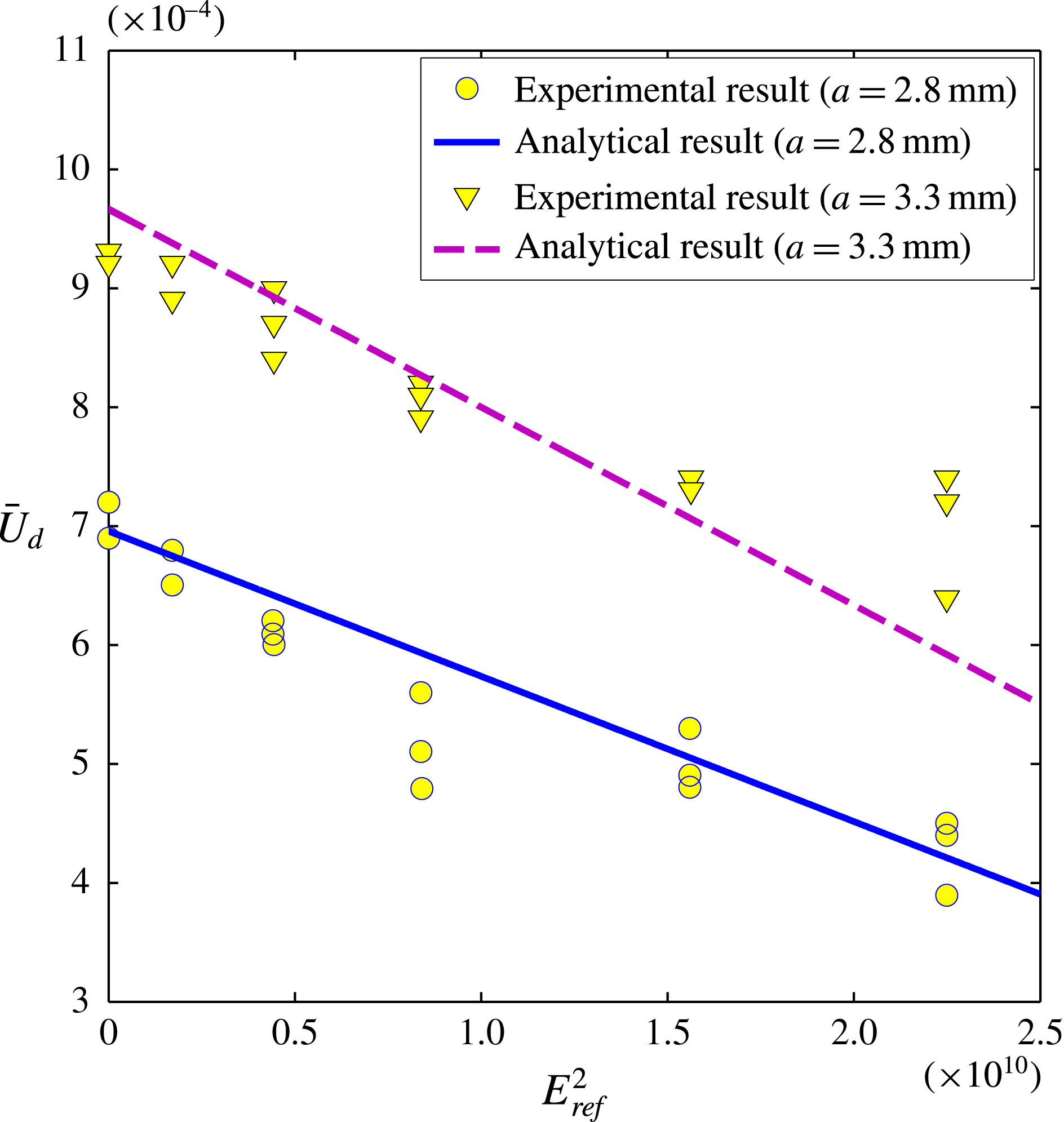
Variation of dimensional drop velocity
 $\bar{U}_{d}\,(\text{m}~\text{s}^{-1})$
with the strength of applied electric field
 $E_{ref}^{2}~(\text{V}^{2}~\text{m}^{-2})$
. Our analytical results are compared with the experimental results of Xu & Homsy (Reference Xu and Homsy2006) for two different drop sizes (
 $a=2.8$
and
 $3.3~\text{mm}$
) over a wide range of the strength of applied electric field. Other parameters as employed by Xu & Homsy (Reference Xu and Homsy2006), have the following values:
 $R=0.6452$
,
 $S=0.35$
,
 ${\it\lambda}=0.357$
,
 ${\it\varepsilon}_{e}=8{\it\varepsilon}_{0}$
,
 ${\it\mu}_{e}=1.4~\text{Pa}~\text{s}$
,
 ${\it\gamma}=5\times 10^{-3}~\text{N}~\text{m}^{-1}$
,
 ${\it\sigma}_{e}=2.4\times 10^{-12}~\text{S}~\text{m}^{-1}$
,
 ${\it\rho}_{i}=1000~\text{kg}~\text{ m}^{-3}$
and
 ${\it\rho}_{e}=957~\text{kg}~\text{m}^{-3}$
.

4 Results and discussion
4.1 Validation
If we consider an applied electric field acting in the
 $z$
-direction, i.e.
 $\boldsymbol{E}_{\infty }=(0,1)$
, we obtain the drop velocity as
 $$\begin{eqnarray}\displaystyle \boldsymbol{U}_{d} & = & \displaystyle \left[1+Re_{E}\left(\frac{6}{5}\frac{M\!\left(S-R\right)(3R-S+3)}{(3+2R)(R+2)^{2}(2+3{\it\lambda})({\it\lambda}+1)}\right)\right.\nonumber\\ \displaystyle & & \displaystyle \left.+\,Ca\left(\frac{3}{20}\frac{M(3{\it\lambda}^{2}-{\it\lambda}+8){\it\Omega}_{T}}{(R+2)^{2}(2+3{\it\lambda})({\it\lambda}+1)}\right)\right]\boldsymbol{e}_{z},\end{eqnarray}$$
which corroborates with the drop sedimentation velocity obtained by Xu & Homsy (Reference Xu and Homsy2006). In figure 2 we compare our analytical results with that of previously reported experimental results of Xu & Homsy (Reference Xu and Homsy2006). They have performed experiments on the measurement of drop velocity in the presence of electric field applied in the direction of gravity for two different drop sizes
 $a=2.8$
and
 $3.3~\text{mm}$
(physical properties are mentioned in the caption). Figure 2 depicts reasonable agreement between theory and experiment.
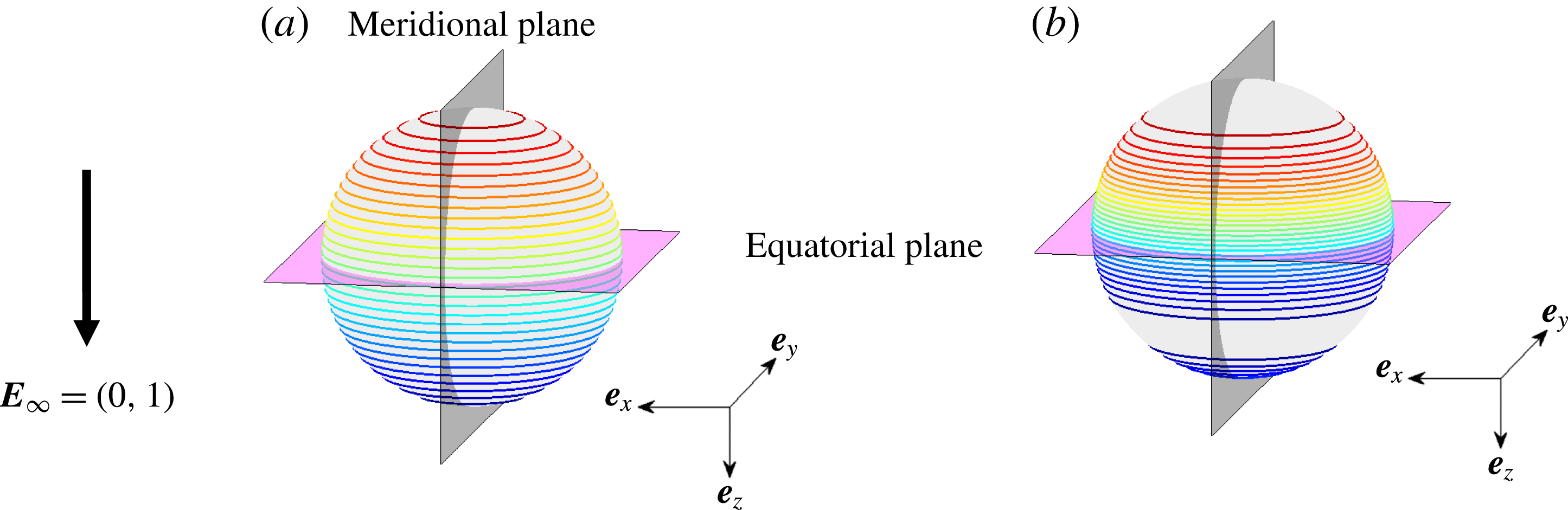
Contours depicting the variation of the (a)
 $q_{s}^{(0)}$
and (b)
 $q_{s}^{(0)}+Re_{E}q_{s}^{(Re_{E})}$
for a longitudinal electric field. The parameters employed are
 $R=0.5,S=2$
,
 $M=2$
,
 ${\it\lambda}=0.5$
and
 $Re_{E}=0.2$
.

4.2 Effect of charge convection and shape deformation on the longitudinal velocity of drop
The drop velocity in the longitudinal direction (
 $z$
-direction) is obtained from (3.36) as
 $$\begin{eqnarray}\displaystyle U_{dz} & = & \displaystyle U_{dz}^{(0)}+Re_{E}U_{dz}^{(Re_{E})}+CaU_{dz}^{(Ca)}\nonumber\\ \displaystyle & = & \displaystyle 1+Re_{E}\left(\frac{3}{10}\frac{M\!\left(S-R\right)(3R-S+3)(4E_{z}^{2}+3E_{x}^{2})}{(3+2R)(R+2)^{2}(2+3{\it\lambda})({\it\lambda}+1)}\right)\nonumber\\ \displaystyle & & \displaystyle +\,Ca\left(\frac{3}{40}\frac{M\!\left(3{\it\lambda}^{2}-{\it\lambda}+8\right)(2E_{z}^{2}-E_{x}^{2}){\it\Omega}_{T}}{(R+2)^{2}\left(2+3{\it\lambda}\right)({\it\lambda}+1)}\right),\end{eqnarray}$$
where
 $U_{dz}^{(0)}=1$
represents the dimensionless Hadamard–Rybcznski velocity,
 $U_{dz}^{(Re_{E})}$
represents the correction in longitudinal drop velocity due to charge convection at the drop surface and
 $U_{dz}^{(Ca)}$
represents the correction in longitudinal drop velocity due to shape deformation of the drop. Before studying the effect of different controlling parameters on the drop velocity, we investigate the physical reasons behind the charge-convection- and shape-deformation-induced alterations in the longitudinal drop velocity.
Regarding the effect of charge convection, previously Feng (Reference Feng1999) showed that despite charge convection, for a neutrally buoyant drop, the charge distribution remains anti-symmetric with respect to the equatorial plane
 $({\it\theta}={\rm\pi}/2)$
of the drop (please refer to figure 3). The consequence of this is that there is no extra force acting on the drop and consequently the drop remains stationary. The problem of a drop with a different density than the suspending fluid in the presence of a longitudinal applied electric field was then considered by Xu & Homsy (Reference Xu and Homsy2006) who highlighted the pivotal role of the surface-charge convection in breaking the antisymmetry about the equatorial plane thus giving rise to a net drag on the drop. This can be seen from figure 3 where we plot (3.8) and (3.21) by setting
 $E_{z}=1$
and
 $E_{x}=0$
. The choice of the parameters used in figure 3 are mentioned in the figure caption. Figure 3(a) depicts the leading-order charge distribution
 $(q_{s}^{(0)})$
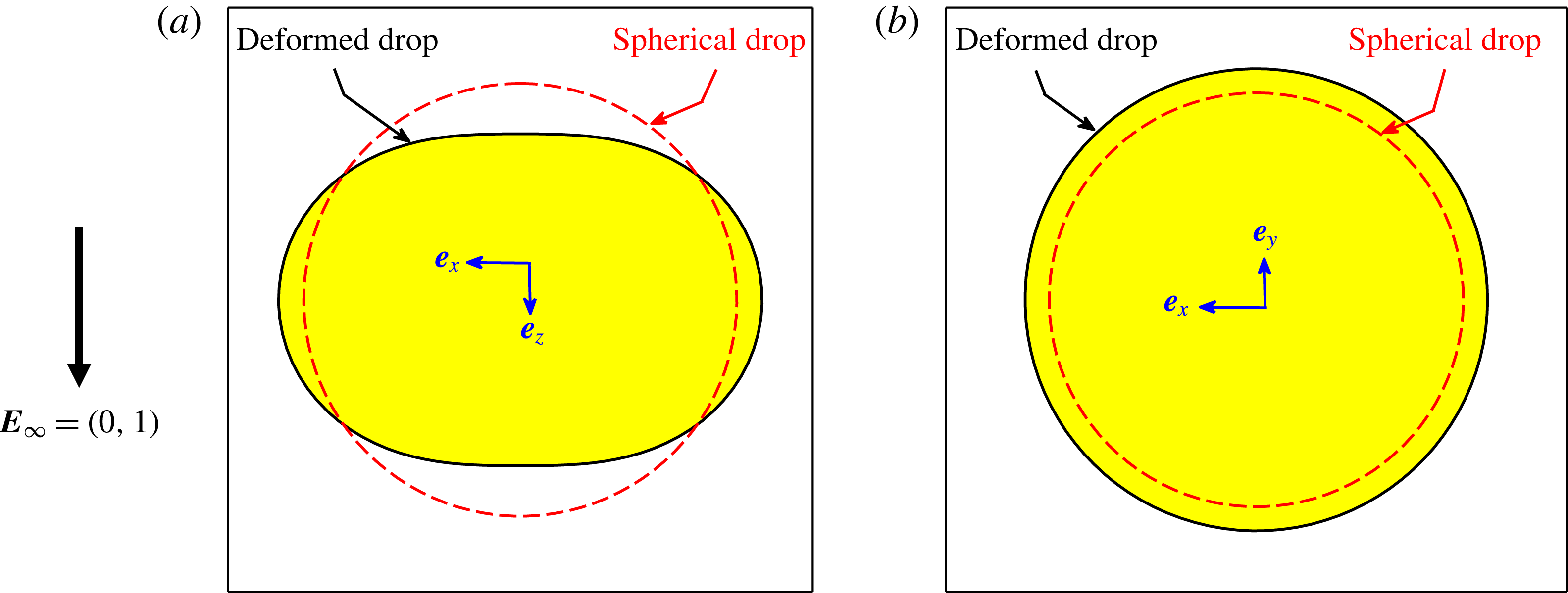
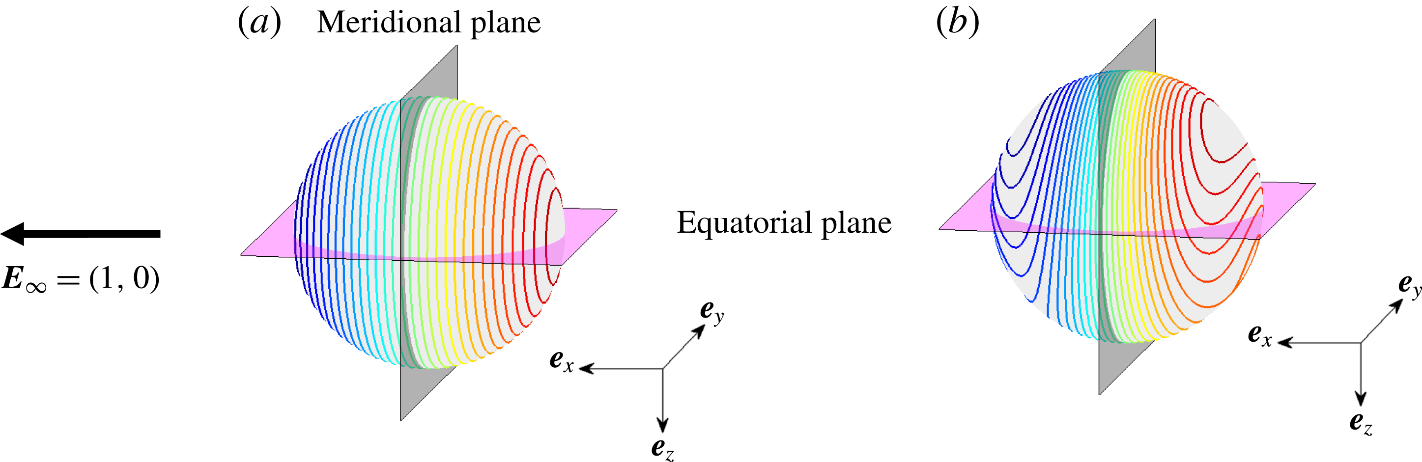
which is antisymmetric about the equatorial plane. However, it can be clearly seen from figure 3(b) that the surface convection for a sedimenting drop does lead to a breaking in the antisymmetric structure of the charge distribution. It is precisely this altered asymmetric charge distribution that results in a non-zero force and subsequently the longitudinal drop velocity. On the other hand, the deformation-induced alteration in longitudinal velocity of the drop is due to the change in drag force on the drop due to change in projected cross-sectional area in the longitudinal direction. In figure 4 we show the shape of the drop in the presence of uniform electric field acting in the longitudinal direction. Figures 4(a) and 4(b) show the extent of drop deformation as compared with the spherical shape in
 $xz$
-plane and
 $xy$
-plane, respectively. From figure 4(b) it is clear that the effective cross-sectional area projected in the direction of sedimentation of the drop due to deformation has increased as compared with the undeformed case, which reduces the drop velocity for the parameters given in the figure caption.
(a) Drop shape projected on the (a)
 $xz$
-plane and (b)
 $xy$
-plane. For the deformed drop shape we have only shown the leading-order deformation. Other parameters employed are
 $R=0.5$
,
 $S=2$
,
 $M=2$
,
 ${\it\lambda}=0.5$
and
 $Ca=0.2$
.

Now, we study the effect of different controlling parameters on the longitudinal velocity of the drop. The most important controlling parameters and non-dimensional numbers which govern the drop velocity are
 $E_{x}$
,
 $E_{z}$
,
 ${\it\lambda}$
,
 $R$
,
 $S$
,
 $M$
,
 $Re_{E}$
and
 $Ca$
. The components of the applied electric field
 $E_{x}$
and
 $E_{z}$
can be represented by an equivalent tilt angle
 $({\it\theta}_{t})$
which is previously defined as
 ${\it\theta}_{t}=\tan ^{-1}(E_{x}/E_{z})$
. Towards investigating the effects of charge convection and shape deformation on the settling velocity of the drop, we show following three cases: drop settling velocity in the absence of deformation
 $(1+Re_{E}U_{dz}^{(Re_{E})})$
, drop settling velocity in the absence of charge convection
 $(1+CaU_{dz}^{(Ca)})$
and finally the combined effect of deformation and charge convection
 $(1+Re_{E}U_{dz}^{(Re_{E})}+CaU_{dz}^{(Ca)})$
. To compare these results with that of sedimentation of drop in the absence of any external electric field, we also plot the
 $U_{dz}=1$
line representing the Hadamard–Rybczynski velocity.
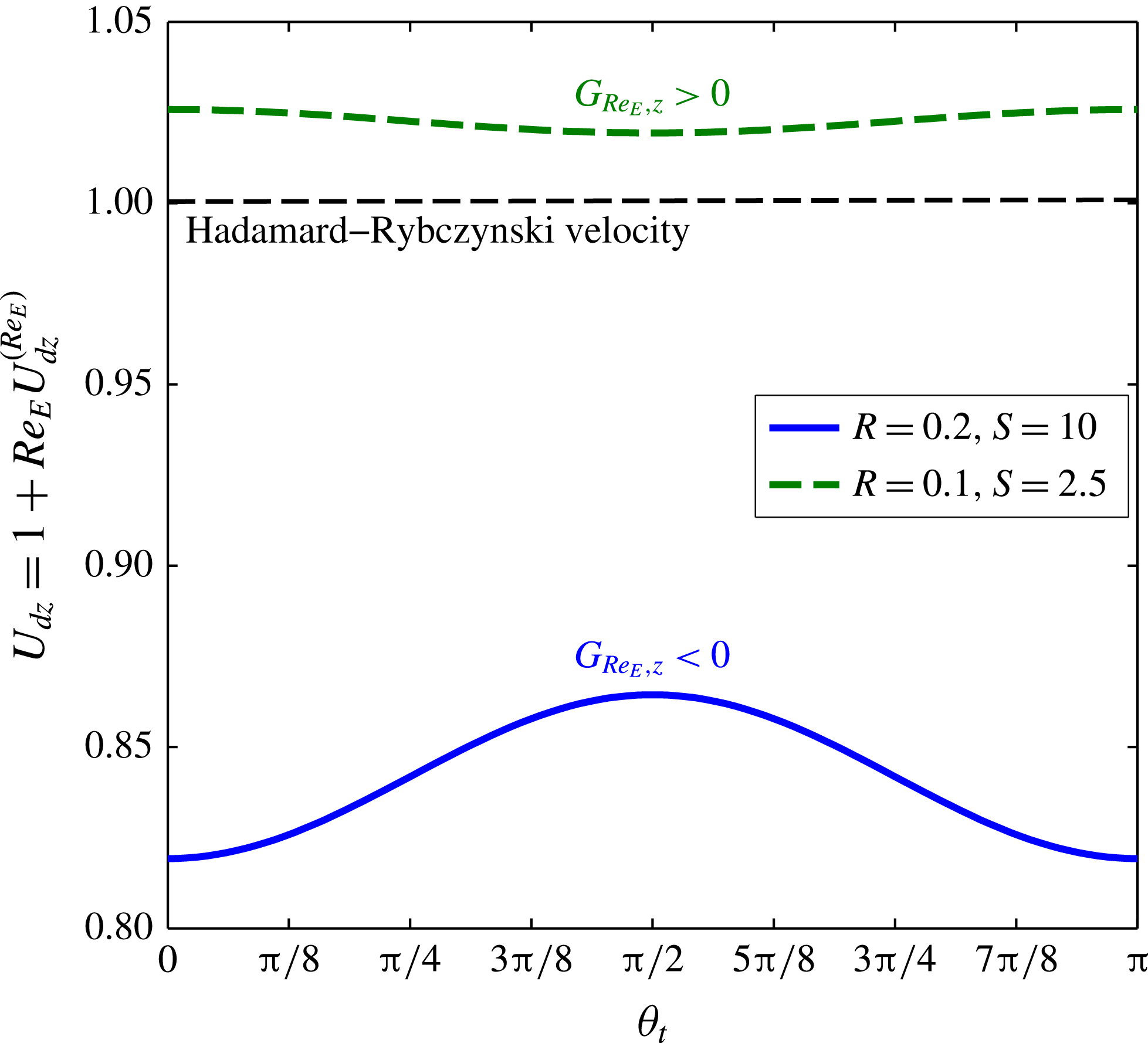
Figure 5 depicts the variation of longitudinal drop velocity with the tilt angle
 $({\it\theta}_{t})$
in the presence of charge convection effect where we deliberately neglect the effects of deformation by setting
 $Ca=0$
. Here we consider two different sets of electrical properties
 $(R,S)$
which are mentioned in the figure caption. It is apparent form figure 5 that charge convection can increase
 $(U_{dz}>1)$
or decrease
 $(U_{dz}<1)$
the longitudinal drop velocity as compared to the Hadamard–Rybczynski velocity
 $(U_{dz}=1)$
. Net effect of charge convection is determined by the sign of the correction term
 $U_{dz}^{(Re_{E})}$
. From (3.29) it is noticeable that the sign of
 $U_{dz}^{(Re_{E})}$
is decided solely by the combination of the conductivity and the permittivity ratio:
 $G_{Re_{E},z}=(S-R)(3R-S+3)$
. If
 $G_{Re_{E},z}<0$
(which is the case for
 $R=0.2$
and
 $S=10$
), the charge convection resists the drop motion in the longitudinal direction, and the reverse happens for
 $G_{Re_{E},z}>0$
(which is the case for
 $R=0.1$
and
 $S=2.5$
). Another important aspect that can be noted from figure 5 is the effect of charge convection towards altering (decrease/increase) the drop velocity in the longitudinal direction which is maximum when
 ${\it\theta}_{t}=0,{\rm\pi}$
and minimum when
 ${\it\theta}_{t}={\rm\pi}/2$
. This is due to the fact that the asymmetry in charge distribution with respect to the equatorial plane is maximum for
 ${\it\theta}_{t}=0,{\rm\pi}$
and minimum for
 ${\it\theta}_{t}={\rm\pi}/2$
.
Variation of drop velocity in the longitudinal direction
 $(U_{dz})$
with tilt angle
 $({\it\theta}_{t})$
for
 $G_{Re_{E}}>0$
and
 $G_{Re_{E}}<0$
. Different parameters considered here have the following values: for
 $G_{Re_{E}}<0$
:
 $R=0.2$
,
 $S=10$
and
 $M=0.5$
, and for
 $G_{Re_{E}}>0$
:
 $R=0.1$
,
 $S=2.5$
and
 $M=2$
. Other parameters have the following values:
 ${\it\lambda}=0.1$
and
 $Re_{E}=0.2$
. The black dashed line represents the
 $U_{dz}=1$
line which is the Hadamard–Rybczynski velocity.

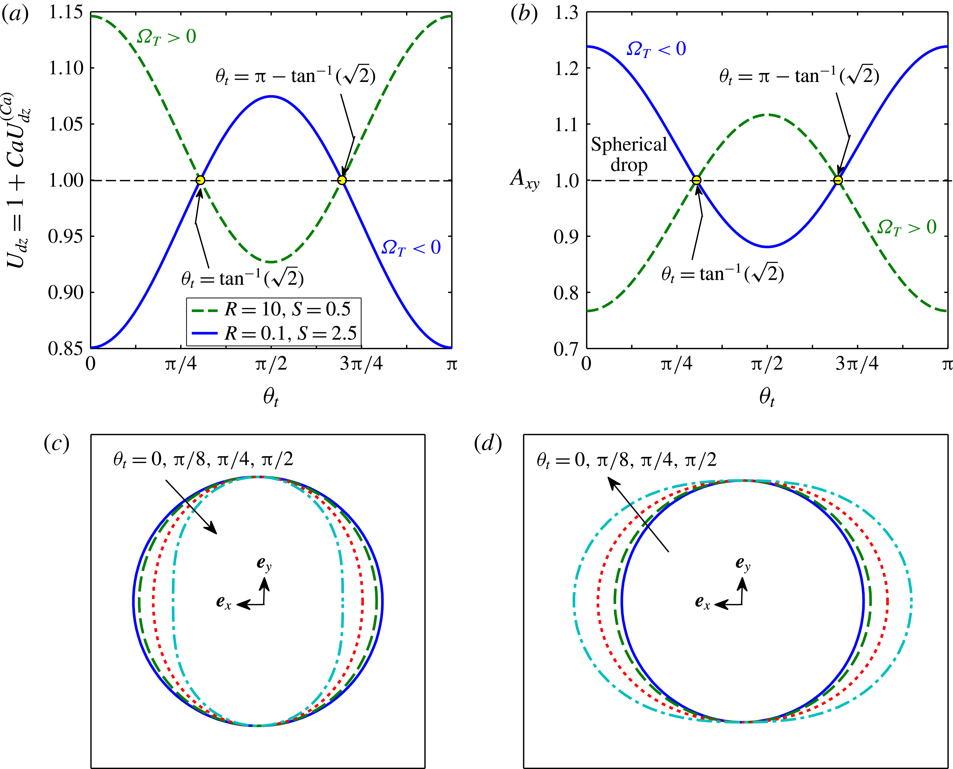
(a) Variation of drop velocity in the longitudinal direction
 $(U_{dz})$
with tilt angle
 $({\it\theta}_{t})$
in the absence of charge convection
 $(Re_{E}=0)$
for
 ${\it\Omega}_{T}<0$
and
 ${\it\Omega}_{T}>0$
. (b) Variation of cross-sectional area of a drop projected on
 $xy$
-plane with tilt angle for
 ${\it\Omega}_{T}<0$
and
 ${\it\Omega}_{T}>0$
. We have normalized
 $A_{xy}$
by
 ${\rm\pi}$
. (c) Cross-sectional area of the deformed drop on the
 $xy$
-plane for
 ${\it\Omega}_{T}<0$
. (d) Cross-sectional area of the deformed drop on the
 $xy$
-plane for
 ${\it\Omega}_{T}>0$
. Different properties used for
 ${\it\Omega}_{T}<0$
are
 $R=0.1$
,
 $S=2.5$
and
 $Ca=0.1$
. Similarly, for
 ${\it\Omega}_{T}>0$
, we have used
 $R=10$
,
 $S=0.5$
and
 $Ca=0.2$
. Other parameters have the following values:
 $M=2$
and
 ${\it\lambda}=0.1$
.

To investigate the pivotal role of drop deformation on the longitudinal velocity of the drop, we plot the longitudinal drop velocity
 $(U_{dz})$
with tilt angle
 $({\it\theta}_{t})$
in the presence of shape deformation effect where we deliberately neglect the effects of charge convection by setting
 $Re_{E}=0$
in figure 6(a). We consider two different cases:
 ${\it\Omega}_{T}<0$
(oblate drop) and
 ${\it\Omega}_{T}>0$
(prolate drop). When the tilt angle is
 ${\it\theta}_{t}=0$
, which is equivalent to the case of
 $\boldsymbol{E}_{\infty }=(0,1),$
the deformation and motion of the drop is exactly axisymmetric about the longitudinal direction which has previously been studied by Xu & Homsy (Reference Xu and Homsy2006). They have reported that a drop in the presence of axial electric field falls slower when
 ${\it\Omega}_{T}<0$
and faster when
 ${\it\Omega}_{T}>0$
. Similar observations are depicted in figure 6(a) for
 ${\it\theta}_{t}=0$
. But with increase in the tilt angle
 $({\it\theta}_{t})$
there is a remarkable change in the drop velocity. For the case of
 ${\it\Omega}_{T}<0$
, the drop velocity increases with the tilt angle and reaches maximum at
 ${\it\theta}_{t}={\rm\pi}/2$
and then decreases. Towards explaining the physical reason behind this behaviour, we appeal to figure 6(b) where we show the effect of tilt angle on the variation of cross-sectional area of the deformed drop projected in the direction of sedimentation
 $(A_{xy})$
. We have normalized the projected cross-section area by the projected area of spherical drop. Figure 6(b) clearly shows that for
 ${\it\Omega}_{T}<0$
(oblate shape) and
 ${\it\theta}_{t}=0$
,
 $A_{xy}>1$
which means a greater cross-sectional area of the deformed drop in the direction of sedimentation which results in greater drag force and subsequently a reduction in drop velocity. With the increase in tilt angle,
 $A_{xy}$
reduces and goes below unity until it reaches a minimum at
 ${\it\theta}_{t}={\rm\pi}/2$
which results in faster sedimentation of the drop as compared with the Hadamard–Rybczynski velocity. For
 ${\rm\pi}/2\leqslant {\it\theta}_{t}\leqslant {\rm\pi}$
,
 $A_{xy}$
increases with
 ${\it\theta}_{t}$
and drop velocity reduces accordingly. The reverse trend is observed for a prolate drop
 $({\it\Omega}_{T}>0)$
for which
 $A_{xy}$
increases and drop velocity reduces with increase in the tilt angle and reaches a minima at
 ${\it\theta}_{t}={\rm\pi}/2$
as shown in figures 6(a) and 6(b). The corresponding drop shapes are shown in figures 6(c) and 6(d) for
 ${\it\Omega}_{T}<0$
and
 ${\it\Omega}_{T}>0$
, respectively, for four different tilt angles
 $({\it\theta}_{t}=0,{\rm\pi}/8,{\rm\pi}/4,{\rm\pi}/2)$
. An important thing to note here is that the sign of
 $U_{dz}^{(Ca)}$
is decided by the parameter
 $G_{Ca,z}=(2E_{z}^{2}-E_{x}^{2}){\it\Omega}_{T}$
. The parameter
 $G_{Ca,z}$
changes sign with tilt angle and there is always two particular values of tilt angle which are
 ${\it\theta}_{t}=\tan ^{-1}(\sqrt{2})$
and
 ${\it\theta}_{t}={\rm\pi}-\tan ^{-1}(\sqrt{2})$
for which
 $U_{dz}^{(Ca)}$
vanishes. The physical reason behind this can be obtained from figure 6(b) which depicts that for
 ${\it\theta}_{t}=\tan ^{-1}(\sqrt{2})(\text{or }{\it\theta}_{t}={\rm\pi}-\tan ^{-1}(\sqrt{2}))$
, the projected cross-sectional area
 $(A_{xy})$
is unity which means there is no effective change in
 $A_{xy}$
as compared with a spherical shape. This is a situation in which the drop deforms but that deformation does not lead to any change in drop velocity in the longitudinal direction.
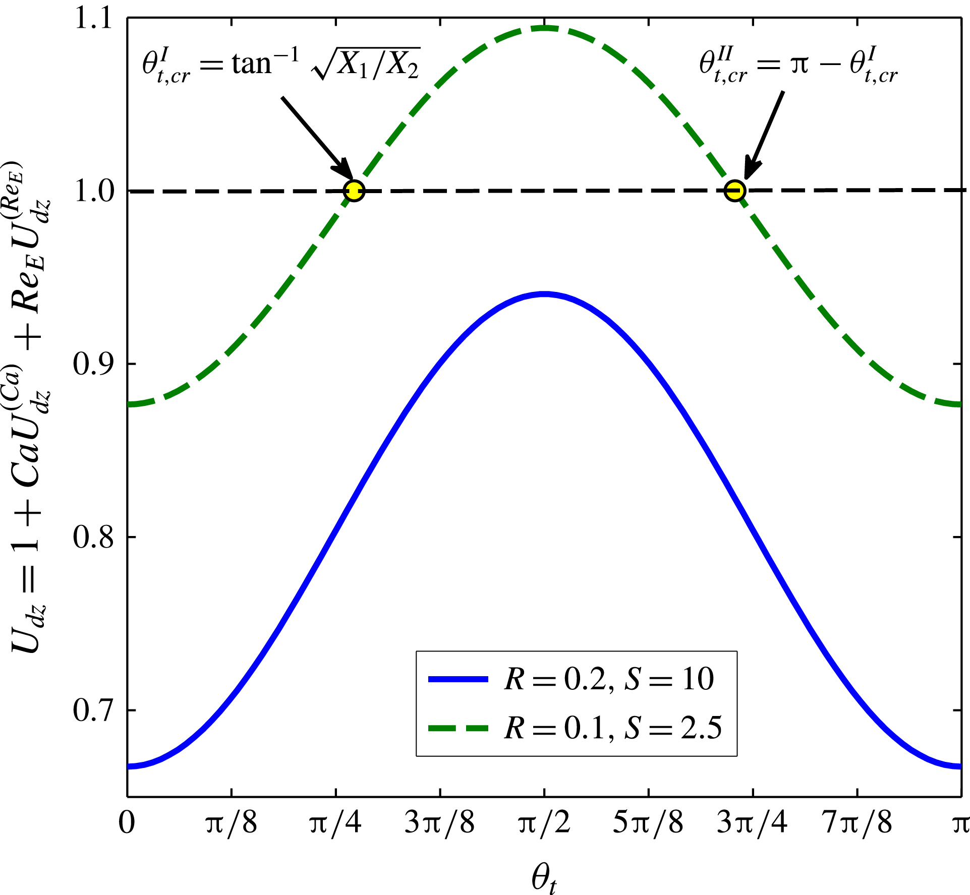
Variation of the drop velocity in the longitudinal direction
 $(U_{dz})$
with tilt angle
 $({\it\theta}_{t})$
for
 $R=0.2$
,
 $S=10$
and
 $M=0.5$
, and for
 $R=0.1$
,
 $S=2.5$
and
 $M=2$
. Other parameters have the following values:
 ${\it\lambda}=0.1$
,
 $Ca=0.1$
and
 $Re_{E}=0.2$
. The black dashed line represents the
 $U_{dz}=1$
line which is the Hadamard–Rybczynski velocity.

Figure 7 depicts that depending on the magnitude of the tilt angle
 $({\it\theta}_{t})$
, the combined effect of charge convection and drop deformation reduce the drop velocity in the longitudinal direction as compared with the Hadamard–Rybczynski velocity for
 $R=0.2$
,
 $S=10$
. But for
 $R=0.1$
,
 $S=2.5$
, figure 7 shows that depending on the tilt angle, the drop velocity may be greater or less than the Hadamard–Rybczynski velocity. Interestingly, figure 7 also shows two critical values of the tilt angle for which the longitudinal velocity of the drop becomes unity
 $(U_{dz}=1)$
. The critical tilt angles are obtained as
 $$\begin{eqnarray}\left.\begin{array}{@{}c@{}}\displaystyle {\it\theta}_{t,cr}^{I}=\tan ^{-1}\left(\sqrt{\frac{X_{1}}{X_{2}}}\right),\\ \displaystyle {\it\theta}_{t,cr}^{\mathit{II}}=\tan ^{-1}\left(-\sqrt{\frac{X_{1}}{X_{2}}}\right)={\rm\pi}-{\it\theta}_{t,cr}^{I},\\ \end{array}\right\}\end{eqnarray}$$
where the terms
 $X_{1}=2[Re_{E}\{(R+1)(32S-24R)-8S(S+1)\}+Ca{\it\Omega}_{T}(2R+3)(3{\it\lambda}^{2}-{\it\lambda}+8)]$
and
 $X_{2}=[Re_{E}\{(R+1)(36R-48S)+12S(S+1)\}+Ca{\it\Omega}_{T}(2R+3)(3{\it\lambda}^{2}-{\it\lambda}+8)].$
It signifies that the longitudinal velocity of the drop remains unaltered for
 ${\it\theta}_{t}={\it\theta}_{t,cr}^{I},{\it\theta}_{t,cr}^{\mathit{II}}$
even in the presence of finite drop deformation
 $(Ca,{\it\Omega}_{T}\neq 0)$
and charge convection
 $(Re_{E}\neq 0)$
. However, this critical tilt angle exists only when
 $X_{1}X_{2}>0$
(which is the case for
 $R=0.1$
,
 $S=2.5$
) depending on the relative magnitude of the electrohydrodynamic parameters
 $(R,S\text{ and }{\it\lambda})$
and non-dimensional numbers
 $(Ca,Re_{E}\text{ and }M)$
.
Variation of the longitudinal velocity of the drop
 $(U_{dz})$
with viscosity ratio
 $({\it\lambda})$
. The parameters have the following values:
 $R=0.2$
,
 $S=10$
,
 ${\it\theta}_{t}={\rm\pi}/8$
,
 $M=0.5$
,
 $Ca=0.1$
and
 $Re_{E}=0.2$
.

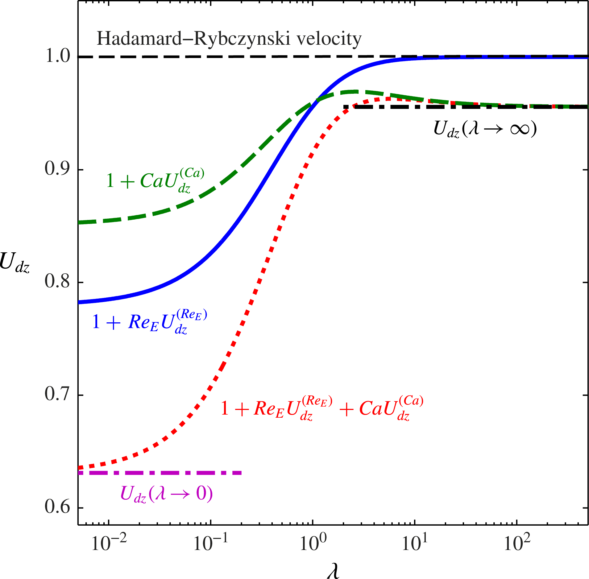
In figure 8 we show the variation of the drop velocity in the longitudinal direction,
 $U_{dz}$
, with viscosity ratio
 $({\it\lambda})$
. Figure 8 depicts that the effect of charge convection reduces monotonically as the drop becomes more viscous and finally becomes negligible as
 ${\it\lambda}\gg 1$
. This can be explained by the fact that with the increase in viscosity ratio, the velocity at the drop surface reduces which leads to a diminishing effect of charge convection in terms of smaller magnitude of
 $U_{dz}^{(Re_{E})}$
. However, the effect of deformation due to electric field persists for high viscosity ratios and contributes to the longitudinal drop velocity. The limit of
 ${\it\lambda}\rightarrow \infty$
, the longitudinal drop velocity reduces to
 $$\begin{eqnarray}U_{dz}({\it\lambda}\rightarrow \infty )=1+Ca\left[\frac{3}{40}\frac{M(2E_{z}^{2}-E_{x}^{2})}{(R+2)^{2}}\left\{R^{2}+1-2S+\frac{9}{5}(R-S)\right\}\right].\end{eqnarray}$$
So for highly viscous drops, alteration of the drop velocity occurs only due to deformation of the drop as depicted in figure 8 and also by (4.4). Another limiting condition is achieved for
 ${\it\lambda}\rightarrow 0$
in which both of the effects, charge convection and deformation, contribute to the drop velocity and yield
 $$\begin{eqnarray}\displaystyle U_{dz}({\it\lambda}\rightarrow 0) & = & \displaystyle \displaystyle \left[1+Re_{E}\biggl[\frac{3}{20}\frac{M\!\left(S-R\right)\left(3R-S+3\right)(4E_{z}^{2}+3E_{x}^{2})}{(3+2R)(R+2)^{2}}\biggr]\right.\nonumber\\ \displaystyle & & \displaystyle \displaystyle \left.+\,Ca\left[\frac{3}{10}\frac{M(2E_{z}^{2}-E_{x}^{2})}{(R+2)^{2}}\left\{R^{2}+1-2S+\frac{6}{5}(R-S)\right\}\right]\right].\end{eqnarray}$$
These two limiting conditions are also shown in figure 8.
We have identified two important parameters
 $G_{Re_{E},z}=(S-R)(3R-S+3)$
and
 $G_{Ca,z}=(2E_{z}^{2}-E_{x}^{2}){\it\Omega}_{T}$
which decide the net effect of charge convection and shape deformation, respectively towards increase/decrease in drop velocity in the
 $z$
-direction. Previously we have shown the importance of the parameter
 $G_{Ca,z}$
in terms of tilt angle
 $({\it\theta}_{t})$
on the direction of motion of the drop in the longitudinal motion. Now we investigate the combined effect of electrical properties
 $(R,S)$
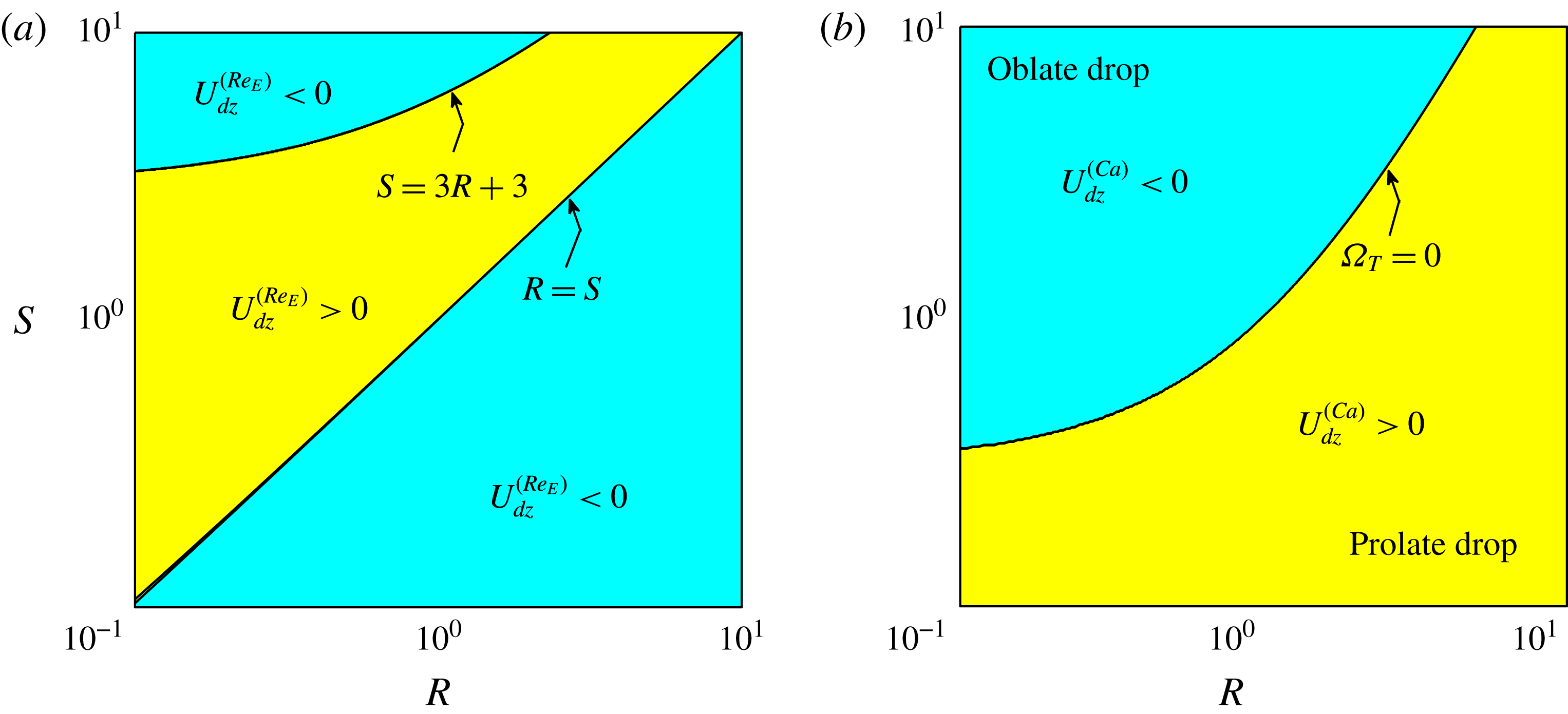
towards determining the longitudinal drop motion. In figures 9(a) and 9(b) we plot the sign of
 $U_{dz}^{(Re_{E})}$
and
 $U_{dz}^{(Ca)}$
, respectively on
 $R$
–
 $S$
plane. Both figures show that there are two distinct regimes on
 $R$
–
 $S$
plane in which the correction in the longitudinal drop velocity becomes positive or negative. In figure 9(a) we identify two regime boundaries given by
 $R=S$
and
 $S=3R+3$
, where the former case is tantamount to a perfect dielectric case with zero surface charge. In figure 9(b) two regimes are distinguished by the zero-deformation line
 $({\it\Omega}_{T}=0)$
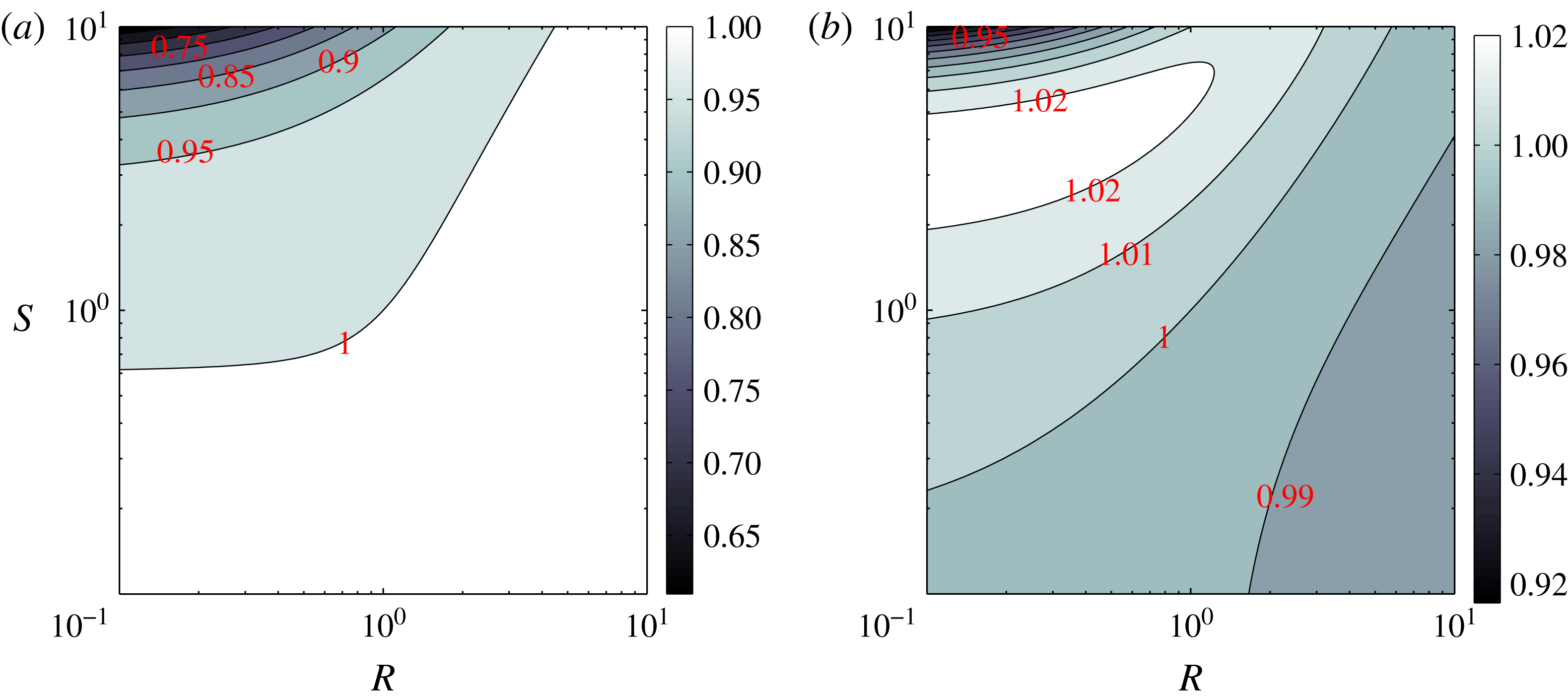
. The correction in the longitudinal velocity due to deformation of the drop is positive for a prolate drop and the reverse is true for oblate drop as depicted in figure 9(b). The combined effect of charge convection and deformation towards dictating the longitudinal motion on the
 $R$
–
 $S$
plane is shown for two different tilt angles in figures 10(a) and 10(b) for fluid properties mentioned in the figure caption. Figure 10(a) depicts that for
 ${\it\theta}_{t}=0$
, there is a marked reduction in the longitudinal drop velocity for small conductivity ratios and large permittivity ratios. The drop velocity remains mostly unaffected for large conductivity ratios. For
 ${\it\theta}_{t}={\rm\pi}/2$
, figure 10(b) depicts that the longitudinal drop velocity is drastically altered as compared with the case of
 ${\it\theta}_{t}=0$
. In sharp contrast to the case of
 ${\it\theta}_{t}=0$
, figure 10(b) shows that drop velocity gets affected for small as well as high conductivity ratios. Another interesting facet is the presence of regions in which the drop velocity is greater that unity which means that the combined effect of charge convection and deformation aids the drop settling.
(a) Different regimes of the correction in longitudinal velocity due to charge convection
 $(U_{dz}^{(Re_{E})})$
. (b) Different regimes of the correction in longitudinal velocity due to drop deformation
 $(U_{dz}^{(Ca)})$
. For the later plot, we have considered
 ${\it\lambda}=0.1$
and
 ${\it\theta}_{t}={\rm\pi}/4$
.

Variation of the longitudinal velocity of drop
 $(U_{dz})$
in
 $R$
–
 $S$
plane for (a)
 ${\it\theta}_{t}=0$
and (b)
 ${\it\theta}_{t}={\rm\pi}/2$
. Other parameters have the following values:
 ${\it\lambda}=0.1$
,
 $M=0.5$
,
 $Ca=0.1$
and
 $Re_{E}=0.2$
. The colourbar and contour levels represent the magnitude of
 $U_{dz}$
.

4.3 Effect of charge convection and shape deformation on the lateral velocity of drop
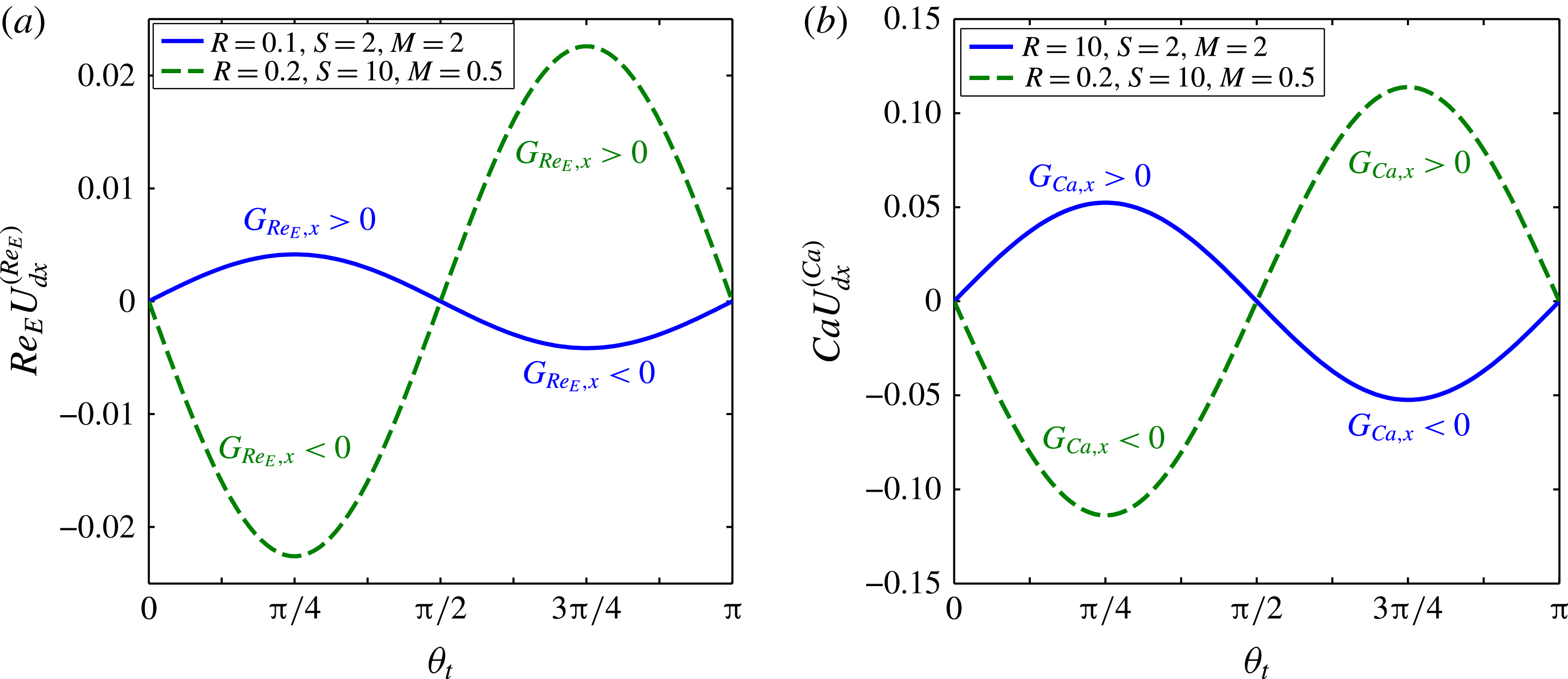
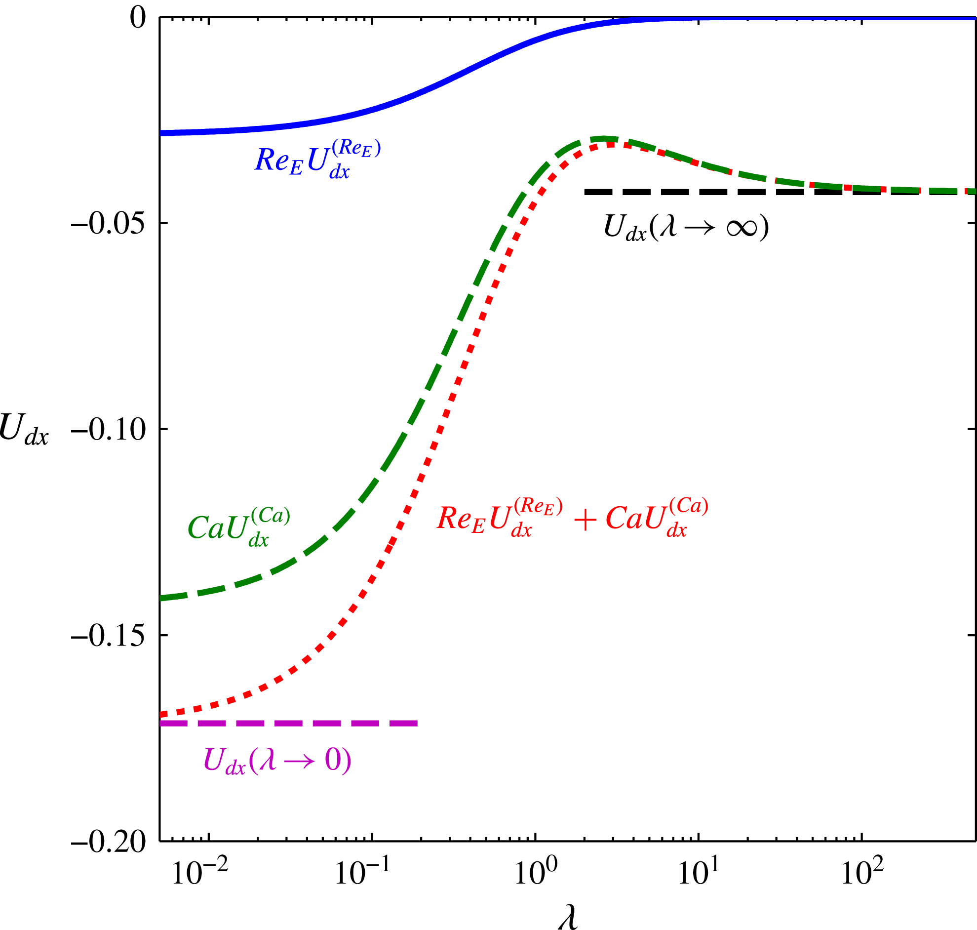
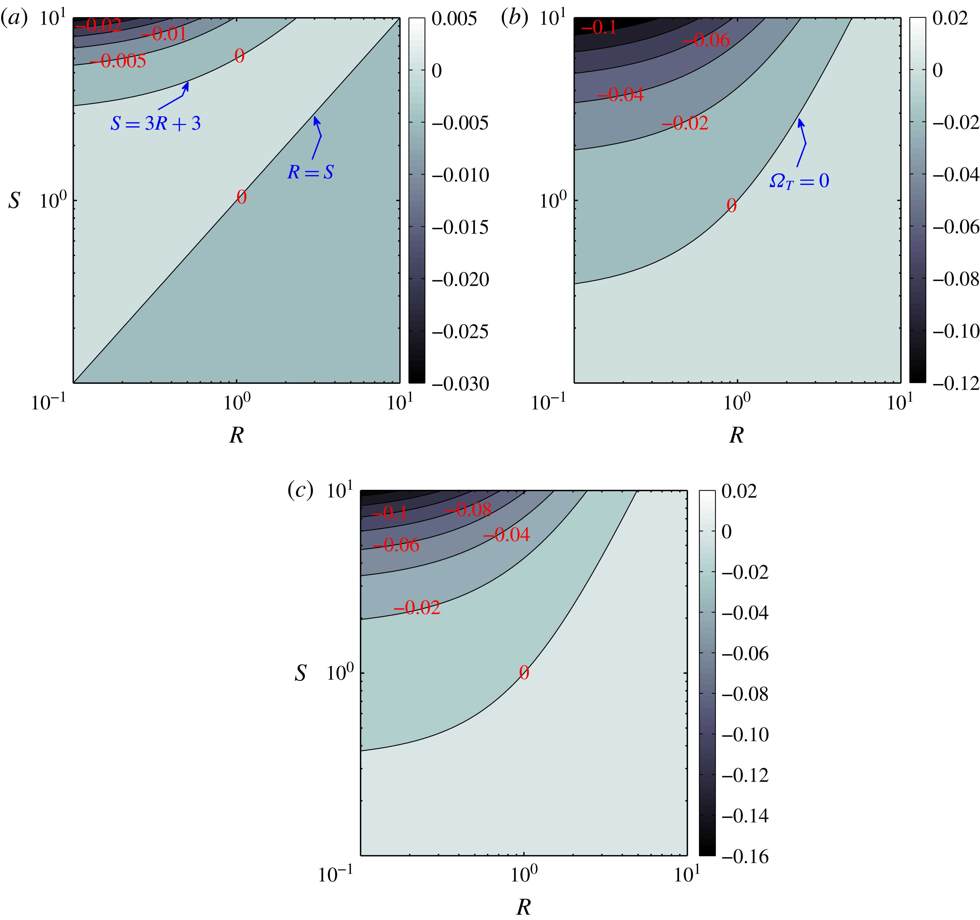
Now we consider the lateral motion of the drop. We had obtained the drop velocity in the lateral direction (
 $x$
-direction) as
 $$\begin{eqnarray}\displaystyle U_{dx} & = & \displaystyle U_{dx}^{(0)}+Re_{E}U_{dx}^{(Re_{E})}+CaU_{dx}^{(Ca)}\nonumber\\ \displaystyle & = & \displaystyle Re_{E}\left(\frac{3}{10}\frac{M(S-R)(3R-S+3)E_{x}E_{z}}{(3+2R)(R+2)^{2}(2+3{\it\lambda})({\it\lambda}+1)}\right)\nonumber\\ \displaystyle & & \displaystyle +\,Ca\left(\frac{9}{40}\frac{M(3{\it\lambda}^{2}-{\it\lambda}+8)E_{x}E_{z}{\it\Omega}_{T}}{(R+2)^{2}(2+3{\it\lambda})({\it\lambda}+1)}\right).\end{eqnarray}$$
This expression depicts that there are two distinct effects contributing to the lateral motion of the drop: charge convection represented by
 $U_{dx}^{(Re_{E})}$
which persists even for a spherical drop and the drop deformation represented by
 $U_{dx}^{(Ca)}$
which remains finite even in the absence of surface charges (the case of perfect dielectric drop in perfect dielectric medium). Before investigating the effect of different controlling parameters on the lateral velocity of the drop, we study the physical reason behind the non-intuitive lateral motion of the drop. One important thing to note here is that the lateral migration obtained in the present analysis is neither due to dielectrophoresis in which the presence of a non-uniform electric field is a must (Feng Reference Feng1996), nor due to electrophoresis in which drop must contain a finite amount of charge (Masliyah & Bhattacharjee Reference Masliyah and Bhattacharjee2006). In the present analysis we obtain lateral migration of the uncharged drop in the presence of a uniform electric field. We first study the charge-convection-induced lateral motion of a spherical drop. We consider the following three cases: (i) longitudinal electric field
 $({\it\theta}_{t}=0)$
, (ii) lateral electric field
 $({\it\theta}_{t}={\rm\pi}/2)$
and (iii) combined longitudinal and lateral fields or equivalently tilted electric field (with
 ${\it\theta}_{t}={\rm\pi}/4$
). The case of a longitudinal electric field has been discussed previously in figure 3. Application of a longitudinal electric field leads to asymmetric charge distribution about the equatorial plane which results in alteration in the drop velocity in the longitudinal direction only. A striking result obtained in (4.6) is that even if there is an applied electric field in lateral direction, the influence of charge convection is solely affecting the longitudinal velocity without causing any motion in the lateral direction. To understand this from the point of view of symmetries in the charge distribution, we appeal to figure 11. It is seen from figure 11(a) that the absence of surface convection leads to an antisymmetric charge distribution about the meridional plane and maintains symmetry about the equatorial plane. In the presence of surface convection due to sedimentation, however, it is observed that the antisymmetric structure is preserved about the meridional plane, but the symmetry is broken about the equatorial plane as depicted in figure 11(b). This leads to a net drag force in the longitudinal direction without affecting the motion in the lateral direction, leading to an alteration in the longitudinal drop velocity. Hence, an applied electric field acting only in the
 $z$
- or
 $x$
-direction (
 ${\it\theta}_{t}=0$
or
 ${\it\theta}_{t}={\rm\pi}/2$
) is insufficient to bring asymmetric charge distribution about the meridional plane due to which there is no velocity of the drop in the lateral direction. Now, we depict the charge distribution due to surface convection in figure 12 where it can be seen that the presence of both components of the applied electric field cause an asymmetry about both the equatorial and meridional plane leading to a force in both the longitudinal and lateral directions, respectively. The findings are also seen in the expressions for the droplet velocity by setting
 $\boldsymbol{E}_{\infty }=(1/\sqrt{2},1/\sqrt{2})$
or equivalently
 ${\it\theta}_{t}={\rm\pi}/4$
in (4.6).
Contours depicting the variation of (a)
 $q_{s}^{(0)}$
and (b)
 $q_{s}^{(0)}+Re_{E}q_{s}^{(Re_{E})}$
for a lateral electric field. The parameters employed are
 $R=0.5$
,
 $S=2$
,
 $M=2$
,
 ${\it\lambda}=0.5$
and
 $Re_{E}=0.2$
.

Contours depicting the variation of
 $q_{s}^{(0)}+Re_{E}q_{s}^{(Re_{E})}$
for a tilted electric field
 $({\it\theta}_{t}={\rm\pi}/4)$
. The parameters employed are
 $R=0.5$
,
 $S=2$
,
 $M=2$
,
 ${\it\lambda}=0.5$
and
 $Re_{E}=0.2$
.

(a) Variation of the drop velocity in the lateral direction
 $(Re_{E}U_{dx}^{(Re_{E})})$
due to charge convection with tilt angle
 $({\it\theta}_{t})$
for the parameters mentioned in the legend. (b) Variation of the drop velocity in the lateral direction due to deformation
 $(CaU_{dx}^{(Ca)})$
with tilt angle
 $({\it\theta}_{t})$
for the parameters mentioned in the legend. Other parameters have the following values:
 ${\it\lambda}=0.1$
,
 $Ca=0.1$
and
 $Re_{E}=0.2$
.

In figure 13(a), we show the variation of
 $Re_{E}U_{dx}^{(Re_{E})}$
with tilt angle for the fluid properties as mentioned in the caption. A closer look into (4.6) reveals that the parameter which governs the direction of the charge-convection-induced lateral motion of the drop can be written as
 $G_{Re_{E},x}=E_{x}E_{z}(S-R)(3R-S+3)=\sin (2{\it\theta}_{t})(S-R)(3R-S+3)/2$
. In contrast to
 $G_{Re_{E},z}$
which is independent of the direction of the applied electric field, here
 $G_{Re_{E},x}$
is markedly altered by the tilt angle
 $({\it\theta}_{t})$
. Depending on the sign of
 $G_{Re_{E},x}$
, the drop can migrate laterally in the positive
 $x$
-direction (for
 $G_{Re_{E},x}>0$
) or in the negative
 $x$
-direction (for
 $G_{Re_{E},x}<0$
). Figure 13(a) depicts the variation of
 $U_{dx}^{(Re_{E})}$
when the tilt angle
 $({\it\theta}_{t})$
is sinusoidal. A few important features that can be noted from figure 13(a) are as follows: (i) charge-convection-induced lateral velocity vanishes for
 ${\it\theta}_{t}=0$
,
 ${\rm\pi}/2$
,
 ${\rm\pi}$
which is due to the fact that for these tilt angles there is no asymmetry in charge distribution with respect to the meridional plane; (ii) charge-convection-induced lateral velocity becomes maximum for
 ${\it\theta}_{t}={\rm\pi}/4$
,
 $3{\rm\pi}/4$
which is due to the fact that the asymmetry in charge distribution with respect to the meridional plane is maximum for
 ${\it\theta}_{t}={\rm\pi}/4$
,
 $3{\rm\pi}/4$
.
In figure 13(b) we plot variation of
 $CaU_{dx}^{(Ca)}$
with the tilt angle
 $({\it\theta}_{t})$
for the properties as mentioned in the caption. Similar to the case of charge convection, the direction of the deformation-induced lateral migration of the drop is determined by the parameter
 $G_{Ca,x}=E_{x}E_{z}{\it\Omega}_{T}=\sin (2{\it\theta}_{t}){\it\Omega}_{T}/2$
. So, the direction of applied electric field and the Taylor discriminating function
 $({\it\Omega}_{T})$
govern the direction of lateral migration due to shape deformation. In this case also we observe sinusoidal behaviour of
 $U_{dx}^{(Ca)}$
with
 ${\it\theta}_{t}$
. Similar to the case of
 $U_{dx}^{(Re_{E})}$
, deformation-induced lateral migration of the drop vanishes at
 ${\it\theta}_{t}=0$
,
 ${\rm\pi}/2$
,
 ${\rm\pi}$
and it becomes maximum at
 ${\it\theta}_{t}={\rm\pi}/4$
,
 $3{\rm\pi}/4$
as depicted in figure 13(b).
In figure 14 we plot the variation of lateral velocity of the drop with viscosity ratio. Similar to the case of longitudinal velocity, with the increase in viscosity ratio, there is a monotonic decrease in charge-convection-induced lateral velocity of the drop because with the increase in viscosity ratio of the drop, the circulations at the drop surface diminishes which subsequently reduces the convection of charges and subsequently the asymmetry in charge distribution as shown in figure 14. The limit of
 ${\it\lambda}\rightarrow \infty$
, the lateral drop velocity reduces to
 $$\begin{eqnarray}U_{dx}({\it\lambda}\rightarrow \infty )=Ca\left[\frac{9}{40}\frac{ME_{x}E_{z}}{(R+2)^{2}}\left\{R^{2}+1-2S+\frac{9}{5}(R-S)\right\}\right].\end{eqnarray}$$
Hence, for highly viscous drops, alteration of drop velocity occurs only due to deformation of the drop as depicted in figure 14 and also by (4.7). Another limiting condition is achieved for
 ${\it\lambda}\rightarrow 0$
in which both of the effects, charge convection and deformation, contribute to the drop velocity and yield
 $$\begin{eqnarray}\displaystyle U_{dx}({\it\lambda}\rightarrow 0) & = & \displaystyle \left[Re_{E}\left[\frac{3}{20}\frac{M(S-R)(3R-S+3)E_{x}E_{z}}{(3+2R)(R+2)^{2}}\right]\right.\nonumber\\ \displaystyle & & \displaystyle +\left.Ca\left[\frac{9}{10}\frac{ME_{x}E_{z}}{(R+2)^{2}}\left\{R^{2}+1-2S+\frac{6}{5}(R-S)\right\}\right]\right].\end{eqnarray}$$
Variation of the lateral velocity of the drop
 $(U_{dx})$
with viscosity ratio
 $({\it\lambda})$
. The parameters have the following values:
 $R=0.2$
,
 $S=10$
,
 ${\it\theta}_{t}={\rm\pi}/4$
,
 $M=0.5$
,
 $Ca=0.1$
and
 $Re_{E}=0.2$
.

Variation of the lateral velocity of the drop
 $(U_{dx})$
in
 $R$
–
 $S$
plane for (a)
 $(Re_{E},Ca)=(0.2,0)$
, (b)
 $(Re_{E},Ca)=(0,0.1)$
and (c)
 $(Re_{E},Ca)=(0.2,0.1)$
. The parameters have the following values:
 ${\it\lambda}=0.1$
,
 $M=0.5$
,
 ${\it\theta}_{t}={\rm\pi}/4$
. The colourbar and contour levels represent the magnitude of
 $U_{dx}$
.

Now, we consider the effects of electrical properties
 $(R,S)$
on the lateral velocity of the drop. The effect of
 $(R,S)$
towards dictating the sign of lateral velocity is the same as that has been shown previously for the longitudinal velocity in figure 9. Here we show the effect of
 $(R,S)$
for
 ${\it\theta}_{t}={\rm\pi}/4$
, since the lateral motion is most significant in this case. In figure 15(a), we plot
 $U_{dx}$
on
 $R$
–
 $S$
plane considering charge convection effect but neglecting the shape deformation of the drop
 $(Ca=0)$
. The effect of drop deformation in the absence of charge convection
 $(Re_{E}=0)$
is shown in figure 15(b), while the combined effect of the charge convection and the shape deformation is depicted in figure 15(c). Figure 15(a–c) depict that depending on the relative magnitudes of conductivity ratio
 $(R)$
and permittivity ratio
 $(S)$
, the lateral velocity of the drop can be in the positive
 $x$
-direction or in the negative
 $x$
-direction. The
 $R=S$
and
 $S=3R+3$
lines are shown to figure 15(a) which signifies the zero lateral velocity of the drop considering charge convection effects. The
 $R=S$
line represents the case of a perfectly dielectric drop having zero surface charge, while
 $S=3R+3$
denotes the zero-lateral-migration line for a leaky dielectric drop. Similar to the case of longitudinal velocity, for the case of
 ${\it\Omega}_{T}=0$
, the deformation-induced motion vanishes in the lateral direction as depicted in figure 15(b).
4.4 Effect of charge convection and deformation on the direction of drop motion
So far we have discussed the effect of charge convection and deformation on the longitudinal and lateral motion of the drop. Here we investigate the combined effect of charge convection and deformation on the direction of motion of the drop; more specifically, the deviation in direction of drop motion form the direction of gravity (
 $z$
-direction). Towards this, we define the deviation angle
 ${\it\theta}_{d}=\tan ^{-1}(U_{dx}/U_{dz})$
which quantifies the angle made by the drop velocity vector,
 $\boldsymbol{U}_{d}$
, with the
 $z$
-direction. When the drop is sedimenting in the positive
 $z$
-direction, the parameters that can affect the direction of drop motion are
 $E_{x}$
and
 $E_{z}$
(or equivalently the tilt angle,
 ${\it\theta}_{t}$
),
 ${\it\lambda}$
,
 $R$
,
 $S$
and the non-dimensional numbers
 $Ca$
,
 $Re_{E}$
and
 $M$
. In figure 16(a,b) we plot variation of the deviation angle
 $({\it\theta}_{d})$
with tilt angle
 $({\it\theta}_{t})$
for the parameters specified in the caption. We consider three different viscosity ratios
 ${\it\lambda}=0.1$
, 1 and 10. Figure 16(a,b) depicts that there is an optimum tilt angle for which magnitude of the deviation angle
 $({\it\theta}_{d})$
is maximum or equivalently the deviation in direction of drop motion from
 $z$
-direction is maximum. Previously we have come across the fact that for specified values of electrical and hydrodynamic properties, the magnitude of lateral velocity of the drop
 $(U_{dx})$
become maximum for
 ${\it\theta}_{t}={\rm\pi}/4$
. However, maximum change in the drop direction may not necessarily take place for
 ${\it\theta}_{t}={\rm\pi}/4$
because the lateral velocity of the drop
 $(U_{dz})$
also changes with the tilt angle
 $({\it\theta}_{t})$
. It is apparent from figure 16(a,b) that viscosity ratio and electrical properties
 $(R,S)$
markedly alter the direction of drop motion. Drops with high viscosity ratios encounter less change in direction of motion (from the impending axial motion) as compared with drops with low viscosity ratios.
Variation of
 ${\it\theta}_{d}$
(in radians) with tilt angle
 $({\it\theta}_{t})$
for (a)
 ${\it\Omega}_{T}>0$
and (b) for
 ${\it\Omega}_{T}<0$
. The parameters considered for
 ${\it\Omega}_{T}>0$
:
 $R=10$
,
 $S=2$
,
 $Ca=0.2$
,
 $Re_{E}=0.2$
,
 $M=2$
and for
 ${\it\Omega}_{T}<0$
:
 $R=0.2$
,
 $S=10$
,
 $Ca=0.1$
,
 $Re_{E}=0.2$
,
 $M=0.5$
. We have considered three different viscosity ratios
 ${\it\lambda}=0.1$
, 1 and 10. The horizontal black dashed line represent the zero lateral migration line
 $({\it\theta}_{d}=0)$
.

Schematic of the experimental set-up. (a) Depicts the front view while (b) represents the side view of the set-up. In the side view, the electrodes are essentially the projections of the electrodes in the front view.

4.5 Experimental investigations
A schematic representation of the experimental set-up is given in figure 17. The set-up consists of an acrylic cell and electrode assembly. The height and width of the acrylic cell are designed as 13 cm each, and the depth is taken as 10 cm. Two brass electrodes attached at the two faces of the container are shown in figure 17. The two faces to which the electrodes are attached are aligned at 45° with regard to the vertical direction. The dimensions of the electrodes are
 $5~\text{cm}\times 7~\text{cm}$
. The thicknesses of the electrodes are 8 mm, and the perpendicular distance between the centres of the faces of the two electrodes is 10 cm. The dimensions are chosen so that the wall effects are minimized (Xu & Homsy Reference Xu and Homsy2006). The edges of the electrodes are rounded to minimize the edge effects related to electric field. The cell is filled with castor oil (Sigma Aldrich) while a drop of silicone oil (AR-10, Sigma Aldrich) is injected manually using a syringe (Dispo Van) from the open top end. For the experiment, the top electrode is energized with high-voltage DC power source using an in-house power supply (High Voltage Laboratory, Department of Electrical Engineering, Indian Institute of Technology Kharagpur) with an output range of 0–20 kV while the bottom electrode is grounded. After the silicone oil drop sediments sufficiently and reaches steady state, the electrodes are energized. The electrodes are ramped up within 20–30 s to the desired voltage level. The voltage is then held constant until the drop migrates sufficient distance and experiences wall effects. The motion of the drop is captured using a Nikon D5200 camera with a Nikon AF NIKKOR 24–85 mm macro lens.
Comparison between experimental and analytical results concerning the droplet deviation angle
 $({\it\theta}_{d})$
for
 ${\it\theta}_{t}={\rm\pi}/4$
and
 $E_{ref}=14.14~\text{kV}$
.

The density and viscosity of the castor oil are
 ${\it\rho}_{e}=959~\text{kg m}^{-3}$
and
 ${\it\mu}_{e}=1~\text{Pa}~\text{s}$
while those of silicone oil are
 ${\it\rho}_{i}=1010~\text{kg m}^{-3}$
and
 ${\it\mu}_{i}=20~\text{mPa}~\text{s}$
. There is no common consensus on the values of the permittivity and conductivity of both the oils (Vizika & Saville Reference Vizika and Saville2006; Xu & Homsy Reference Xu and Homsy2006). Castor oil has a high propensity to absorb moisture and hence has a wide range of permittivity values, while silicone oil has a very sensitive dependence of the conductivity on the ambient temperature (Xu & Homsy Reference Xu and Homsy2006). The values of the conductivities and relative permittivities for both the oils are considered as (Vizika & Saville Reference Vizika and Saville2006; Xu & Homsy Reference Xu and Homsy2006; Salipante & Vlahovska Reference Salipante and Vlahovska2010):
 ${\it\sigma}_{e}=10^{-11}~\text{S m}^{-1}$
and
 ${\it\varepsilon}_{e}=2.6$
for castor oil, and
 ${\it\sigma}_{i}=10^{-12}~\text{S m}^{-1}$
and
 ${\it\varepsilon}_{i}=2.9$
for silicone oil. For a 2 mm diameter silicone oil drop we obtain the non-dimensional numbers as:
 $Ca=0.165$
,
 $Re_{E}=0.38$
and
 $M=2.787$
. The combined effect of deformation and charge convection on the drop deviation angle
 $({\it\theta}_{d})$
is given in figure 18, corresponding to a DC voltage of 14.14 kV. These results can be put in the perspective of the main contention of the analysis presented in the manuscript that is based on the claim that the presence of a tilted uniform electric field is responsible for causing lateral migration of an otherwise sedimenting drop: a phenomenon which is absent in either of the cases of a vertically applied electric field or a horizontally applied electric field. The experimental results clearly reveal that the presence of a tilted electric field (here
 ${\it\theta}_{t}={\rm\pi}/4$
) is responsible for the lateral migration of the drop.
5 Conclusions
To summarize, we have obtained analytical expressions for the velocity of a sedimenting drop in the presence of a uniform electric field acting in an arbitrary direction, considering small shape deformation and small charge convection effects. Drop deformation and charge convection independently contribute to the alteration in drop velocity in both the longitudinal as well as lateral directions. Experimental measurements also confirm the lateral migration of the drop in the presence of tilted electric field. Several interesting conclusions that can be drawn from the present analysis are as follows.
-
(i) Drop deformation can increase/decrease the velocity in the longitudinal direction depending on the sign of the parameter
$G_{Ca,z}=(2E_{z}^{2}-E_{x}^{2}){\it\Omega}_{T}$
. The relative strength of the components of applied electric field
$(E_{x},E_{z})$
, or equivalently the tilt angle
$({\it\theta}_{t})$
, significantly alters the deformation-induced longitudinal motion of the drop. For
${\it\theta}_{t}=\tan ^{-1}(\sqrt{2})$
or
${\rm\pi}-\tan ^{-1}(\sqrt{2})$
, the deformation-induced correction in longitudinal velocity of the drop vanishes. Deformation aids the longitudinal motion of the drop for
$0\leqslant {\it\theta}_{t}<\tan ^{-1}(\sqrt{2})$
and
${\rm\pi}-\tan ^{-1}(\sqrt{2})<{\it\theta}_{t}<{\rm\pi}$
, and resists the same for
$\tan ^{-1}(\sqrt{2})<{\it\theta}_{t}<{\rm\pi}-\tan ^{-1}(\sqrt{2})$
when the drop shape is prolate
$({\it\Omega}_{T}>0)$
. The reverse happens for oblate drops
$({\it\Omega}_{T}<0)$
. -
(ii) Charge convection can increase/decrease the drop velocity in the longitudinal direction depending on the sign of the parameter
$G_{Re_{E},z}=(S-R)(3R-S+3)$
. Charge convection increases the longitudinal drop velocity for
$G_{Re_{E},z}>0$
and decreases the same for
$G_{Re_{E},z}<0$
. -
(iii) Combined effect of charge convection and shape deformation on the longitudinal drop velocity not only depends on the relative magnitude of
$Re_{E}$
and
$Ca$
, but also significantly changes with the tilt angle
$({\it\theta}_{t})$
. We obtain there may exist two values of the tilt angles (
${\it\theta}_{t,cr}^{I}$
and
${\it\theta}_{t,cr}^{II}$
) for which
$U_{dz}=1$
. -
(iv) Both charge convection and shape deformation may induce lateral motion of the drop depending on the electrohydrodynamic properties (
$R$
,
$S$
and
${\it\lambda}$
) and the tilt angle
$({\it\theta}_{t})$
. The tilt angle dramatically alters the drop velocity in the lateral direction. The lateral velocity of the drop is maximum for
${\it\theta}_{t}={\rm\pi}/4$
,
$3{\rm\pi}/4$
but vanishes for
${\it\theta}_{t}=0$
,
${\rm\pi}/2$
,
${\rm\pi}$
. Hence, the necessary condition for non-zero lateral velocity of the drop can be given by
$0<{\it\theta}_{t}<{\rm\pi}/2$
or
${\rm\pi}/2<{\it\theta}_{t}<{\rm\pi}$
. -
(v) Charge-convection-induced lateral motion of the drop takes place in the positive (or negative)
$x$
-direction when
$G_{Re_{E},x}=E_{x}E_{z}(S-R)(3R-S+3)>0$
(or
$G_{Re_{E},x}<0$
), whereas deformation-induced lateral motion of the drop takes place in the positive (or negative)
$x$
-direction when
$G_{Ca,x}=E_{x}E_{z}{\it\Omega}_{T}>0$
(or
$G_{Ca,x}<0$
). -
(vi) An increase in viscosity ratio always reduces the effect of charge convection and the deformation. For highly viscous drops, the effect of charge convection diminishes and the motion of the drop is governed by the deformation only.
-
(vii) A spherical drop (the case of large surface tension) can experience change in velocity in both longitudinal and lateral directions due to the charge convection at the drop surface.
-
(viii) A perfectly dielectric drop (the case of
$R=S$
) experiences a change in velocity in both longitudinal and lateral direction due to deformation.

















Acknowledgements
The authors A.B. and S.C. would like to acknowledge funding from SRIC, IIT Kharagpur under the Project ‘Centre of Excellence for Training and Research in Microfluidics’. The authors would like to acknowledge Mr A. Sarkar and Mr S. K. Naskar for fabrication of the acrylic cell and brass electrodes. The authors also acknowledge the time and efforts of Mr R. Paul, Mr G. Naveen Kumar, Mr T. S. Roy and Mr B. Sarkar for assistance in performing the experiments.
Supplementary material
Supplementary material is available at http://dx.doi.org/10.1017/jfm.2016.84.
Appendix A. Expressions of the solid harmonics present in the Lamb’s general solution
The solid harmonics present in the Lamb’s general solution (3.2)–(3.5) have the following form (Hetsroni & Haber Reference Hetsroni and Haber1970).
The growing solid harmonics
 $p_{n}^{(k)},{\it\Phi}_{n}^{(k)}$
and
 ${\it\chi}_{n}^{(k)}$
are given by
 $$\begin{eqnarray}\left.\begin{array}{@{}c@{}}\displaystyle p_{n}^{(k)}={\it\lambda}r^{n}\mathop{\sum }_{m=0}^{n}[A_{n,m}^{(k)}\cos (m{\it\phi})+\hat{A}_{n,m}^{(k)}\sin (m{\it\phi})]P_{n,m},\\ \displaystyle {\it\Phi}_{n}^{(k)}=r^{n}\mathop{\sum }_{m=0}^{n}[B_{n,m}^{(k)}\cos (m{\it\phi})+\hat{B}_{n,m}^{(k)}\sin (m{\it\phi})]P_{n,m},\\ \displaystyle {\it\chi}_{n}^{(k)}=r^{n}\mathop{\sum }_{m=0}^{n}[C_{n,m}^{(k)}\cos (m{\it\phi})+{\hat{C}}_{n,m}^{(k)}\sin (m{\it\phi})]P_{n,m},\end{array}\right\}\end{eqnarray}$$
and the decaying solid spherical harmonics
 $p_{-n-1}^{(k)},{\it\Phi}_{-n-1}^{(k)}$
and
 ${\it\chi}_{-n-1}^{(k)}$
are given by
 $$\begin{eqnarray}\left.\begin{array}{@{}c@{}}\displaystyle p_{-n-1}^{(k)}=r^{-n-1}\mathop{\sum }_{m=0}^{n}[A_{-n-1,m}^{(k)}\cos (m{\it\phi})+\hat{A}_{-n-1,m}^{(k)}\sin (m{\it\phi})]P_{n,m},\\ \displaystyle {\it\Phi}_{-n-1}^{(k)}=r^{-n-1}\mathop{\sum }_{m=0}^{n}[B_{-n-1,m}^{(k)}\cos (m{\it\phi})+\hat{B}_{-n-1,m}^{(k)}\sin (m{\it\phi})]P_{n,m},\\ \displaystyle {\it\chi}_{-n-1}^{(k)}=r^{-n-1}\mathop{\sum }_{m=0}^{n}[C_{-n-1,m}^{(k)}\cos (m{\it\phi})+{\hat{C}}_{-n-1,m}^{(k)}\sin (m{\it\phi})]P_{n,m}.\end{array}\right\}\end{eqnarray}$$
In (A 1) and (A 2),
 $A_{n,m}^{(k)}$
,
 $B_{n,m}^{(k)}$
,
 $C_{n,m}^{(k)}$
,
 $A_{-n-1,m}^{(k)}$
,
 $B_{-n-1,m}^{(k)}$
and
 $C_{-n-1,m}^{(k)}$
are the unknowns to be obtained using appropriate boundary conditions.
Appendix B. Expressions of the solid harmonics present in the velocity and pressure fields at leading order
The growing solid harmonics present in (3.9) and (3.10) are of the following form
 $$\begin{eqnarray}\left.\begin{array}{@{}rcl@{}}{\it\Phi}_{1}^{(0)}\, & =\, & rB_{1,0}^{(0)}P_{1,0},\\ {\it\Phi}_{2}^{(0)}\, & =\, & r^{2}[B_{2,0}^{(0)}P_{2,0}+B_{2,1}^{(0)}\cos {\it\phi}P_{2,1}+B_{2,2}^{(0)}\cos (2{\it\phi})P_{2,2}],\\ p_{1}^{(0)}\, & =\, & {\it\lambda}rA_{1,0}^{(0)}P_{1,0},\\ p_{2}^{(0)}\, & =\, & {\it\lambda}r^{2}[A_{2,0}^{(0)}P_{2,0}+A_{2,1}^{(0)}\cos {\it\phi}P_{2,1}+A_{2,2}^{(0)}\cos (2{\it\phi})P_{2,2}],\end{array}\right\}\end{eqnarray}$$
where the coefficients
 $A^{(0)}$
and
 $B^{(0)}$
are obtained as
 $$\begin{eqnarray}\left.\begin{array}{@{}c@{}}\displaystyle A_{1,0}^{(0)}=-\frac{5}{{\it\lambda}+1},\quad A_{2,0}^{(0)}=-\frac{63}{10}(E_{x}^{2}-2E_{z}^{2}){\it\Lambda},\quad A_{2,1}^{(0)}=\frac{63}{5}E_{x}E_{z}{\it\Lambda},\\ \displaystyle A_{2,2}^{(0)}=\frac{63}{20}E_{x}^{2}{\it\Lambda},\quad B_{1,0}^{(0)}=\frac{1}{2({\it\lambda}+1)},\quad B_{2,0}^{(0)}=\frac{9}{20}(E_{x}^{2}-2E_{z}^{2}){\it\Lambda},\\ \displaystyle B_{2,1}^{(0)}=-{\textstyle \frac{9}{10}}E_{x}E_{z}{\it\Lambda},\quad B_{2,2}^{(0)}=-{\textstyle \frac{9}{40}}E_{x}^{2}{\it\Lambda},\end{array}\right\}\end{eqnarray}$$
where the parameter
 ${\it\Lambda}$
is given by
 ${\it\Lambda}=M(R-S)/({\it\lambda}+1)(R+2)^{2}$
. The decaying solid harmonics present in (3.11) and (3.12) are of the following form
 $$\begin{eqnarray}\left.\begin{array}{@{}rcl@{}}\displaystyle {\it\Phi}_{-2}^{(0)}\, & =\, & {\displaystyle \frac{1}{r^{2}}}B_{-2,0}^{(0)}P_{1,0},\\ \displaystyle p_{-2}^{(0)}\, & =\, & {\displaystyle \frac{1}{r^{2}}}[A_{-2,0}^{(0)}P_{1,0}+A_{-2,1}^{(0)}\cos {\it\phi}P_{1,1}+\hat{A}_{-2,1}^{(0)}\sin {\it\phi}P_{1,1}],\\ \displaystyle {\it\Phi}_{-3}^{(0)}\, & =\, & {\displaystyle \frac{1}{r^{3}}}[B_{-3,0}^{(0)}P_{2,0}+B_{-3,1}^{(0)}\cos {\it\phi}P_{2,1}+B_{-3,2}^{(0)}\cos (2{\it\phi})P_{2,2}],\\ \displaystyle p_{-3}^{(0)}\, & =\, & {\displaystyle \frac{1}{r^{3}}}[A_{-3,0}^{(0)}P_{2,0}+A_{-3,1}^{(0)}\cos {\it\phi}P_{2,1}+A_{-3,2}^{(0)}\cos (2{\it\phi})P_{2,2}],\end{array}\right\}\end{eqnarray}$$
where the coefficients
 $A^{(0)}$
and
 $B^{(0)}$
are obtained as
 $$\begin{eqnarray}\displaystyle \left.\begin{array}{@{}c@{}}\displaystyle A_{-2,0}^{(0)}=\frac{(2+3{\it\lambda})U_{dz}^{(0)}}{2({\it\lambda}+1)},\quad A_{-2,1}^{(0)}=\frac{(2+3{\it\lambda})U_{dx}^{(0)}}{2({\it\lambda}+1)},\quad \hat{A}_{-2,1}^{(0)}=\frac{(2+3{\it\lambda})U_{dy}^{(0)}}{2({\it\lambda}+1)},\\ \displaystyle A_{-3,0}^{(0)}=-{\textstyle \frac{9}{5}}(E_{x}^{2}-2E_{z}^{2}){\it\Lambda},\quad A_{-3,1}^{(0)}={\textstyle \frac{18}{5}}E_{x}E_{z}{\it\Lambda},\quad A_{-3,2}^{(0)}={\textstyle \frac{9}{10}}E_{x}^{2}{\it\Lambda},\end{array}\right\} & & \displaystyle\end{eqnarray}$$
 $$\begin{eqnarray}\displaystyle \left.\begin{array}{@{}c@{}}\displaystyle B_{-2,0}^{(0)}=\frac{{\it\lambda}}{4({\it\lambda}+1)},\quad B_{-3,0}^{(0)}=-\frac{3}{10}(E_{x}^{2}-2E_{z}^{2}){\it\Lambda},\quad B_{-3,1}^{(0)}=\frac{3}{5}E_{x}E_{z}{\it\Lambda},\\ B_{-3,2}^{(0)}={\textstyle \frac{3}{20}}E_{x}^{2}{\it\Lambda}.\end{array}\right\} & & \displaystyle\end{eqnarray}$$
Appendix C. Complete expressions of
$Z$
present at the right-hand side of the charge conservation equation at
$O(Re_{E})$


The complete expressions of the non-zero
 $Z_{n,m}$
are obtained as
 $$\begin{eqnarray}\left.\begin{array}{@{}rclrcl@{}}\,\displaystyle Z_{1,0}\, & =\, & {\displaystyle \frac{54}{25}}{\displaystyle \frac{M(R-S)^{2}E_{z}}{(R+2)^{3}({\it\lambda}+1)}}, & Z_{1,1}\, & =\, & {\displaystyle \frac{54}{25}}{\displaystyle \frac{M(R-S)^{2}E_{x}}{(R+2)^{3}({\it\lambda}+1)}},\\ \,\displaystyle Z_{2,0}\, & =\, & -{\displaystyle \frac{3(R-S)E_{z}}{(R+2)({\it\lambda}+1)}}, & Z_{2,1}\, & =\, & -{\displaystyle \frac{3}{2}}{\displaystyle \frac{(R-S)E_{x}}{(R+2)({\it\lambda}+1)}},\\ \,\displaystyle Z_{3,0}\, & =\, & -{\displaystyle \frac{216}{25}}{\displaystyle \frac{M(R-S)^{2}E_{z}}{(R+2)^{3}({\it\lambda}+1)}}, & Z_{3,1}\, & =\, & -{\displaystyle \frac{216}{25}}{\displaystyle \frac{M(R-S)^{2}E_{x}}{(R+2)^{3}({\it\lambda}+1)}},\\ \,\displaystyle Z_{3,2}\, & =\, & {\displaystyle \frac{54}{25}}{\displaystyle \frac{M(R-S)^{2}E_{z}E_{x}^{2}}{(R+2)^{3}({\it\lambda}+1)}}, & Z_{3,3}\, & =\, & {\displaystyle \frac{9}{25}}{\displaystyle \frac{M(R-S)^{2}E_{x}^{3}}{(R+2)^{3}({\it\lambda}+1)}}.\end{array}\right\}\end{eqnarray}$$
Appendix D. Expressions of the coefficients present in the
$O(Re_{E})$
electric field

The non-zero coefficients in the
 $O(Re_{E})$
electric potential in (3.19) and (3.20) are obtained as
 $$\begin{eqnarray}\left.\begin{array}{@{}c@{}}\displaystyle a_{1,0}^{(Re_{E})}=\frac{Z_{1,0}}{2+R},\quad a_{1,1}^{(Re_{E})}=\frac{Z_{1,1}}{2+R},\quad a_{2,0}^{(Re_{E})}=\frac{Z_{2,0}}{3+2R},\quad a_{2,1}^{(Re_{E})}=\frac{Z_{2,1}}{3+2R},\\ \displaystyle a_{3,0}^{(Re_{E})}=\frac{Z_{3,0}}{4+3R},\quad a_{3,1}^{(Re_{E})}=\frac{Z_{3,1}}{4+3R},\quad a_{3,2}^{(Re_{E})}=\frac{Z_{3,2}}{4+3R},\quad a_{3,3}^{(Re_{E})}=\frac{Z_{3,3}}{4+3R},\\ b_{-2,0}^{(Re_{E})}=a_{1,0}^{(Re_{E})},\quad b_{-2,1}^{(Re_{E})}=a_{1,1}^{(Re_{E})},\quad b_{-3,0}^{(Re_{E})}=a_{2,0}^{(Re_{E})},\quad b_{-3,1}^{(Re_{E})}=a_{2,1}^{(Re_{E})},\\ b_{-4,0}^{(Re_{E})}=a_{3,0}^{(Re_{E})},\quad b_{-4,1}^{(Re_{E})}=a_{3,1}^{(Re_{E})},\quad b_{-4,2}^{(Re_{E})}=a_{3,2}^{(Re_{E})},\quad b_{-4,3}^{(Re_{E})}=a_{3,3}^{(Re_{E})}.\end{array}\right\}\end{eqnarray}$$
Appendix E. Expressions of the coefficients present in the
$O(Ca)$
electric field

The non-zero coefficients in the
 $O(Ca)$
electric potential in (3.30) and (3.31) are obtained as
 $$\begin{eqnarray}\left.\begin{array}{@{}c@{}}\displaystyle a_{1,0}^{(Ca)}=\frac{9(1-R)}{5(R+2)^{2}}[3E_{x}L_{2,1}^{(Ca)}+2E_{z}L_{2,0}^{(Ca)}],\\ \displaystyle a_{1,1}^{(Ca)}=\frac{9(1-R)}{5(R+2)^{2}}[3E_{z}L_{2,1}^{(Ca)}-E_{x}L_{2,0}^{(Ca)}+6E_{x}L_{2,2}^{(Ca)}],\\ \displaystyle a_{3,0}^{(Ca)}=0,\quad a_{3,1}^{(Ca)}=0,\quad a_{3,2}^{(Ca)}=0,\quad a_{3,3}^{(Ca)}=0,\\ \displaystyle b_{-2,0}^{(Ca)}=\frac{3(R-1)^{2}}{5(R+2)^{2}}[3E_{x}L_{2,1}^{(Ca)}+2E_{z}L_{2,0}^{(Ca)}],\\ \displaystyle b_{-2,1}^{(Ca)}=\frac{3(R-1)^{2}}{5(R+2)^{2}}[3E_{z}L_{2,1}^{(Ca)}-E_{x}L_{2,0}^{(Ca)}+6E_{x}L_{2,2}^{(Ca)}],\\ \displaystyle b_{-4,0}^{(Ca)}=\frac{9(1-R)}{5(R+2)}[E_{x}L_{2,1}^{(Ca)}-E_{z}L_{2,0}^{(Ca)}],\quad \displaystyle b_{-4,1}^{(Ca)}=\frac{3(1-R)}{5(R+2)}[E_{x}L_{2,2}^{(Ca)}-2E_{z}L_{2,1}^{(Ca)}-E_{x}L_{2,0}^{(Ca)}],\\ \displaystyle b_{-4,2}^{(Ca)}=\frac{3(R-1)}{10(R+2)}[E_{x}L_{2,1}^{(Ca)}+2E_{z}L_{2,2}^{(Ca)}],\quad \displaystyle b_{-4,3}^{(Ca)}=\frac{3(R-1)}{10(R+2)}E_{x}L_{2,2}^{(Ca)}.\end{array}\right\}\end{eqnarray}$$