

1 Introduction
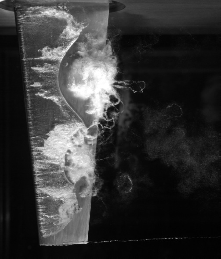
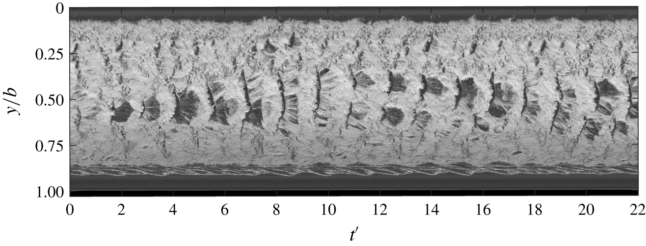
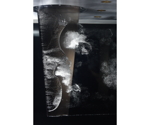
The increasing importance of flow-induced vibrations over time is being driven by advancements in materials technology and ever increasing optimisation, resulting in structures becoming lighter, more flexible and susceptible to vibrations (Blevins Reference Blevins1977). Flow-induced vibration phenomena have a profound influence on the performance of the vast range of aerodynamic and hydrodynamic objects and are therefore significant in geometrical and structural design (Bisplinghoff, Ashley & Halfman Reference Bisplinghoff, Ashley and Halfman1955). Cavitation about a hydrofoil involves a range of complex dynamical phenomena including mass transfer via phase change and diffusion, shockwaves, large- and small-scale instabilities and turbulence, some of which are discernible in figure 1. These phenomena have the potential to cause significant and destructive vibrations (Franc & Michel Reference Franc and Michel2004). Understanding these fluid–structure interaction (FSI) phenomena is of interest as flow over a lifting body can significantly alter the performance of maritime propulsion and control systems.
Cloud cavitation about a finite-span stainless steel hydrofoil exhibiting multiple shedding events along the span due to the re-entrant jet instability and spanwise compatibility of the cavitation. The hydrofoil is vertically mounted at an incidence of  $6^{\circ }$ to the flow with
 $Re=0.8\times 10^{6}$ and
 $\unicode[STIX]{x1D70E}=0.7$.

Experimental studies investigating the influence of cavitation on flexible (i.e. compliant) hydrofoils has previously been conducted by Kaplan & Lehman (Reference Kaplan and Lehman1966), Brennen, Oey & Babcock (Reference Brennen, Oey and Babcock1980), Ausoni et al. (Reference Ausoni, Farhat, Escaler, Egusquiza and Avellan2007) and Ducoin, Astolfi & Sigrist (Reference Ducoin, Astolfi and Sigrist2012) with Kaplan & Lehman (Reference Kaplan and Lehman1966) first observing modest vibration amplitudes due to cavitation about a hydrofoil. Examining the coupling between the hydro-elasticity and the trailing-edge vortex cavitation, Ausoni et al. (Reference Ausoni, Farhat, Avellan, Escaler and Egusquiza2005, Reference Ausoni, Farhat, Escaler, Egusquiza and Avellan2007) observed that not only does the cavitation influence the structural vibrations, but the structural vibrations also affect cavitation behaviour. Numerical simulations by Akcabay & Young (Reference Akcabay and Young2014) modelling the bending and torsional compliance of a cantilevered hydrofoil revealed maximum force and deflection fluctuations occurred when the maximum cavity length approaches the trailing edge. Additionally, hydrofoil compliance was seen to increase the cavity length, thus decreasing the cavitation shedding frequency. However, the influence of compliance was only significant when the cavity length was near the trailing edge. The unsteady two-phase flow has effect on the spectral content of a compliant hydrofoil compared to a relatively stiff one, causing frequency modulation (Akcabay & Young Reference Akcabay and Young2015), broadening of the frequency content (Akcabay et al. Reference Akcabay, Chae, Young, Ducoin and Astolfi2014) and leading to phenomena such as lock-in that lead to significant amplification of vibrations (Kato, Dan & Matsudaira Reference Kato, Dan and Matsudaira2006; Akcabay & Young Reference Akcabay and Young2015).
Cloud cavitation was first extensively investigated by Knapp (Reference Knapp1955) where the detachment of a vapour cloud from an attached cavity due to a re-entrant jet was observed. Since then, several mechanisms have been identified as potential instabilities causing periodic shedding, depending on the flow conditions, in a particular streamwise pressure gradient. These included growth of interfacial instabilities such as Kelvin–Helmholtz waves (Brennen Reference Brennen1969; Avellan, Dupont & Ryhming Reference Avellan, Dupont and Ryhming1988; Brandner et al. Reference Brandner, Walker, Niekamp and Anderson2010), re-entrant jet formation (Furness & Hutton Reference Furness and Hutton1975; Le, Franc & Michel Reference Le, Franc and Michel1993; Kawanami et al. Reference Kawanami, Kato, Yamaguchi, Tanimura and Tagaya1997; Stutz & Reboud Reference Stutz and Reboud1997; Pham, Larrarte & Fruman Reference Pham, Larrarte and Fruman1999; Callenaere et al. Reference Callenaere, Franc, Michel and Riondet2001; Laberteaux & Ceccio Reference Laberteaux and Ceccio2001a,Reference Laberteaux and Cecciob; Smith et al. Reference Smith, Venning, Giosio, Brandner, Pearce and Young2017, Reference Smith, Venning, Brandner, Pearce, Giosio and Young2018, Reference Smith, Venning, Giosio, Brandner, Pearce and Young2019) and shock propagation (Jakobsen Reference Jakobsen1964; Reisman, Wang & Brennen Reference Reisman, Wang and Brennen1998; Ganesh, Mäkiharju & Ceccio Reference Ganesh, Mäkiharju and Ceccio2016; Smith et al. Reference Smith, Venning, Brandner, Pearce, Giosio and Young2018). In certain conditions, multiple instabilities can be present simultaneously with Ganesh et al. (Reference Ganesh, Mäkiharju and Ceccio2016) showing both bubbly shock propagation and re-entrant jet flow from measurements of the void fraction field with X-ray densiotmetry. In addition, Brandner et al. (Reference Brandner, Walker, Niekamp and Anderson2010), and more recently de Graaf, Brandner & Pearce (Reference de Graaf, Brandner and Pearce2017), using high-speed photography observed all three mechanisms either occurring in isolation or as a complex, coupled mechanism in cloud cavitation about a sphere. Furthermore, experiments on a NACA0015 hydrofoil revealed complex multi-stage shedding cycles involving both re-entrant jet and shockwave instabilities (Venning et al. Reference Venning, Smith, Brandner, Giosio and Pearce2017, Reference Venning, Giosio, Smith, Bryce and Brandner2018b).
A re-entrant jet forms by flow over the cavity interface forming an instantaneous stagnation on the wall associated with the cavity closure, resulting in some flow directed back upstream along the hydrofoil surface (Brennen Reference Brennen1995). The re-entrant jet travels upstream towards the cavity detachment until it impinges upon and breaks up the cavity surface, resulting in a detached cavity that is advected downstream as a bubbly mixture, termed a ‘cloud’ structure due to its similarity in visual appearance. As mentioned previously, the re-entrant jet shedding mechanism has been extensively studied and it has been found that for re-entrant jet-driven cloud cavitation to occur, the cavity needs to close in a region with a sufficiently large adverse pressure gradient as well as being thick enough to limit interaction between the re-entrant jet and the cavity interface (Franc Reference Franc2001). Cloud cavitation driven by the re-entrant jet instability, referred to as Type II oscillation in the literature, has a shedding frequency that is dependent on the cavity length, and therefore  $\unicode[STIX]{x1D70E}$ as well as incidence,
 $\unicode[STIX]{x1D6FC}$ (Callenaere et al. Reference Callenaere, Franc, Michel and Riondet2001). In the case of a hydrofoil, the cavity closes in a reducing adverse pressure gradient as it grows and approaches the trailing edge. This leads to degradation of the re-entrant jet and a transition of the primary instability driving shedding to a shockwave instability (Kjeldsen & Arndt Reference Kjeldsen and Arndt2001).
As the attached cavity grows on a hydrofoil, a change in the shedding mechanism is observed with the re-entrant jet instability transitioning to a shockwave instability. Shockwave-driven cloud cavitation, referred to as Type I oscillations (Kjeldsen & Arndt Reference Kjeldsen and Arndt2001), occurs when a reduction in  $\unicode[STIX]{x1D70E}$ or increase in
 $\unicode[STIX]{x1D6FC}$ causes increased cavity size and significant reduction in local void fraction to allow shockwave formation and propagation from the collapse of bubbles. For shockwave formation and propagation, the shed clouds need to be densely populated with bubbles that interact and collapse coherently (Reisman et al. Reference Reisman, Wang and Brennen1998). Additionally, the sound speed of the liquid–vapour mixture is required to fall below the local flow speed (Ganesh et al. Reference Ganesh, Mäkiharju and Ceccio2016; Wu, Ganesh & Ceccio Reference Wu, Ganesh and Ceccio2019). This can occur under cavitating conditions as the presence of bubbles increases the local void fraction which has been shown to significantly reduce the speed of sound in the bubbly mixture (Shamsborhan et al. Reference Shamsborhan, Coutier-Delgosha, Caignaert and Nour2010). These conditions are met when the cavity has increased in size to shed large-scale vapour structures that raise the local void fraction sufficiently.
To reduce the complexity of the cavitation dynamics in three-dimensional (3-D) flows, a large number of past studies have focused on two-dimensional (2-D) flows. However, even in the 2-D case, the resulting shedding physics still exhibit significant 3-D characteristics, as observed by Kubota et al. (Reference Kubota, Kato, Yamaguchi and Maeda1989), de Lange & de Bruin (Reference de Lange and de Bruin1998) and Kawanami, Kato & Yamaguchi (Reference Kawanami, Kato and Yamaguchi1998), resulting in spanwise variations of the cloud cavitation. Furthermore, Kawanami et al. (Reference Kawanami, Kato and Yamaguchi1998) show that cloud cavitation can have a spanwise spatial periodicity on a 2-D hydrofoil where periodic shedding occurs at multiple locations along the span, depending on the streamwise length of the cavity. This is also observed by Prothin, Billard & Djeridi (Reference Prothin, Billard and Djeridi2016) and Smith et al. (Reference Smith, Venning, Brandner, Pearce, Giosio and Young2018, Reference Smith, Venning, Giosio, Brandner, Pearce and Young2019) showing multiple stable shedding locations along a finite-span hydrofoil, highlighting the role of compatibility between the cavity length and the span first noted by Kawanami et al. (Reference Kawanami, Kato and Yamaguchi1998). In both 2-D and 3-D flows, incompatible cavity lengths are seen to result in incoherent shedding along the span (Kawanami et al. Reference Kawanami, Kato and Yamaguchi1998; Kjeldsen, Arndt & Effertz Reference Kjeldsen, Arndt and Effertz2000; Smith et al. Reference Smith, Venning, Brandner, Pearce, Giosio and Young2018; Harwood et al. Reference Harwood, Felli, Falchi, Garg, Ceccio and Young2019). The formation of stable shedding sites is seen to be reinforced by the spanwise component of shedding mechanisms, such as re-entrant jets, as they prevent other instabilities from interfering in the local shedding process (de Lange & de Bruin Reference de Lange and de Bruin1998).
Investigations into the effect of hydrofoil planform geometry by Ihara, Watanabe & Shizukuishi (Reference Ihara, Watanabe and Shizukuishi1989) have shown sweep to minimise lift and drag force fluctuations associated with the absence of large cavity break-off that is observed on an unswept hydrofoil. Furthermore, the highly swept hydrofoil is seen to confine full-chord cloud cavitation to the downstream portion of the hydrofoil, with the upstream portion forming a stable cavity. This cavitation behaviour is due to the strong spanwise flow component redirecting the re-entrant jet away from the cavity detachment, thus preventing cavity break-off and allowing a stable cavity to form Laberteaux & Ceccio (Reference Laberteaux and Ceccio2001b). Time-resolved particle image velocimetry experiments on a 3-D hydrofoil by Foeth et al. (Reference Foeth, Van Doorne, Van Terwisga and Wieneke2006) also shows significant cavitation stability sensitivity due to 3-D flow effects. The influence on cloud cavitation of a free tip, tapered planform and spanwise cavity oscillations remain largely to be investigated, despite several investigations into the effect of a varying spanwise geometry.
This research consists of two parts and is devoted to understanding the influence of FSI on cloud cavitation about a hydrofoil. Cavitating conditions are achieved about the vertically mounted cantilevered hydrofoil through precise pressure control of the variable-pressure water tunnel. Forces acting on the hydrofoil were acquired simultaneously with tip deflections and cavitation behaviour measurements using high-speed photography at various cavitation regimes by varying the free-stream water tunnel pressure. The results produce further insight and correlation between the shedding physics, hydrofoil loading and structural deformations. Part 1 is dedicated to establishing a reference through utilising a relatively stiff hydrofoil whereby the deformations are small compared to the dimensions. Hence, the structural dynamics of the hydrofoil has minimal effect on the loading and cavity dynamics. Part 2 (Smith et al. Reference Smith, Venning, Pearce, Young and Brandner2020) investigates the influence of FSI by utilising a compliant hydrofoil with observations informed by those made on the relatively stiff reference in Part 1.
2 Experimental overview
2.1 Experimental facility
Measurements were undertaken at the Australian Maritime College in the Cavitation Research Laboratory variable-pressure water tunnel. The tunnel test section measures 0.6 m square by 2.6 m long in which the operating velocity and absolute pressure can be varied from  $2$ to
 $12~\text{m}~\text{s}^{-1}$ and 4 to 400 kPa, respectively. The medium sized tunnel contains
 $365~\text{m}^{3}$ of demineralised water. While there is a permanent background nuclei population present in the water, these are of sufficiently high strength and sparsity to be considered inactive in this flow (Venning et al. Reference Venning, Khoo, Pearce and Brandner2018c). The circuit architecture has been developed for continuous elimination of nuclei achieved through a combination of coalescence/gravity separation in a downstream tank and dissolution via extended residence in a resorber (Brandner Reference Brandner2018). This allows consistent long duration measurements as the oncoming recirculated flow is free from nuclei produced from the cavitating hydrofoil that might influence the cavitation behaviour, as observed by Arndt & Keller (Reference Arndt and Keller2003) and Russell et al. (Reference Russell, Venning, Brandner, Pearce, Giosio and Ceccio2018). A detailed description of the facility is given in Brandner, Lecoffre & Walker (Reference Brandner, Lecoffre and Walker2007).
Measurements were taken at a fixed incidence,  $\unicode[STIX]{x1D6FC}$, of
 $6^{\circ }$ and a chord-based Reynolds number,
 $Re=U_{\infty }\bar{c}/\unicode[STIX]{x1D708}$, equal to
 $0.8\times 10^{6}$, where
 $\bar{c}$ is the mean chord,
 $U_{\infty }$ is the free-stream velocity and
 $\unicode[STIX]{x1D708}$ is the kinematic viscosity of the water. The cavitation number,
 $\unicode[STIX]{x1D70E}=2(p_{\infty }-p_{v})/\unicode[STIX]{x1D70C}U_{\infty }^{2}$, where
 $p_{\infty }$ is the absolute static pressure at the level of the hydrofoil tip,
 $p_{v}$ is the vapour pressure and
 $\unicode[STIX]{x1D70C}$ is the water density, was incrementally varied from
 $1.2$ to
 $0.2$ to investigate various cavitation regimes. Dissolved oxygen levels were kept between 3 and 4 ppm for all measurements.
2.2 Model hydrofoil
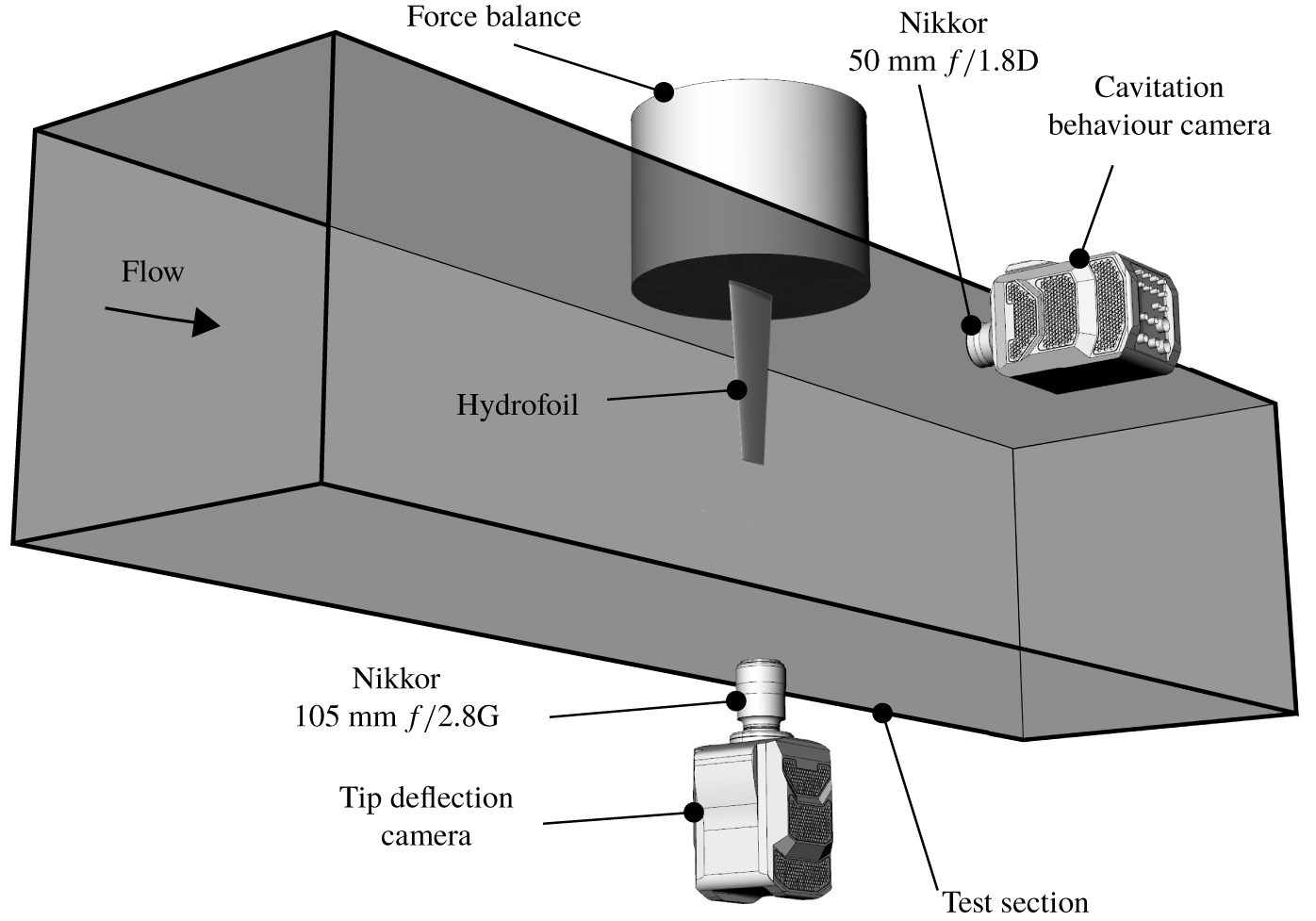
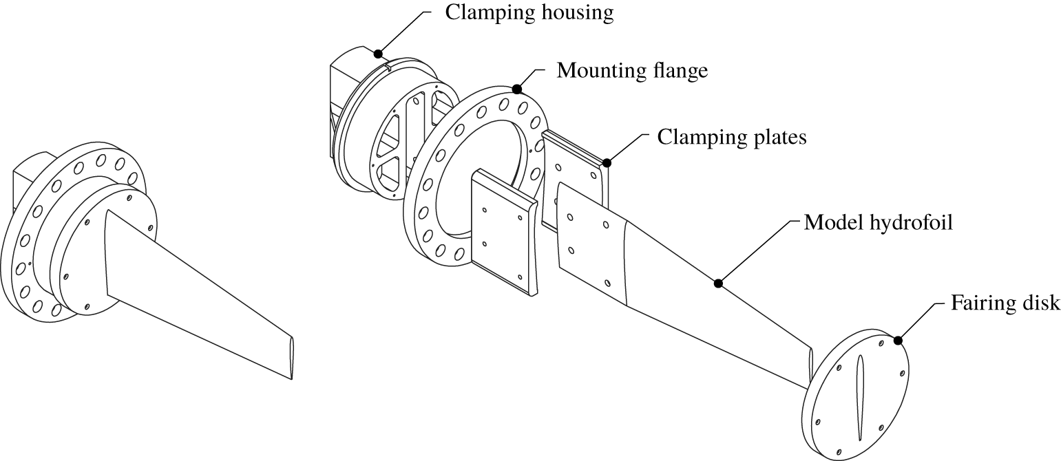
The model hydrofoil was mounted vertically on the centreline, 1.3 m downstream of the test section entrance through a 160 mm diameter penetration in the ceiling. A schematic of the experimental set-up is shown in figure 2. The hydrofoil was attached to a six-component force balance, with an estimated precision of  $0.1\,\,\%$, via a housing which clamped the hydrofoil into place using two profiled plates (figure 3). The penetration is made fair (to
 $50~\unicode[STIX]{x03BC}\text{m}$) using an acrylic disk mounted to the measurement side of the force balance. The fairing disk has a
 $0.5$ mm radial clearance to avoid interference with the force measurement. This type of mounting arrangement was implemented to accommodate the manufacturing of composite models used in Part 2 and to ensure common fixed-end conditions for comparative measurements between the stainless steel and composite models (Zarruk et al. Reference Zarruk, Brandner, Pearce and Phillips2014).
Experimental set-up whereby the hydrofoil is attached to a force balance and mounted vertically on the test section ceiling. Cavitation behaviour and tip deflections were recorded using high-speed photography utilising two Phantom v2640 high-speed cameras mounted on the side and below the test section, respectively.

Hydrofoil model assembly showing an exploded view of the clamping housing arrangement that allows continuity of the model.

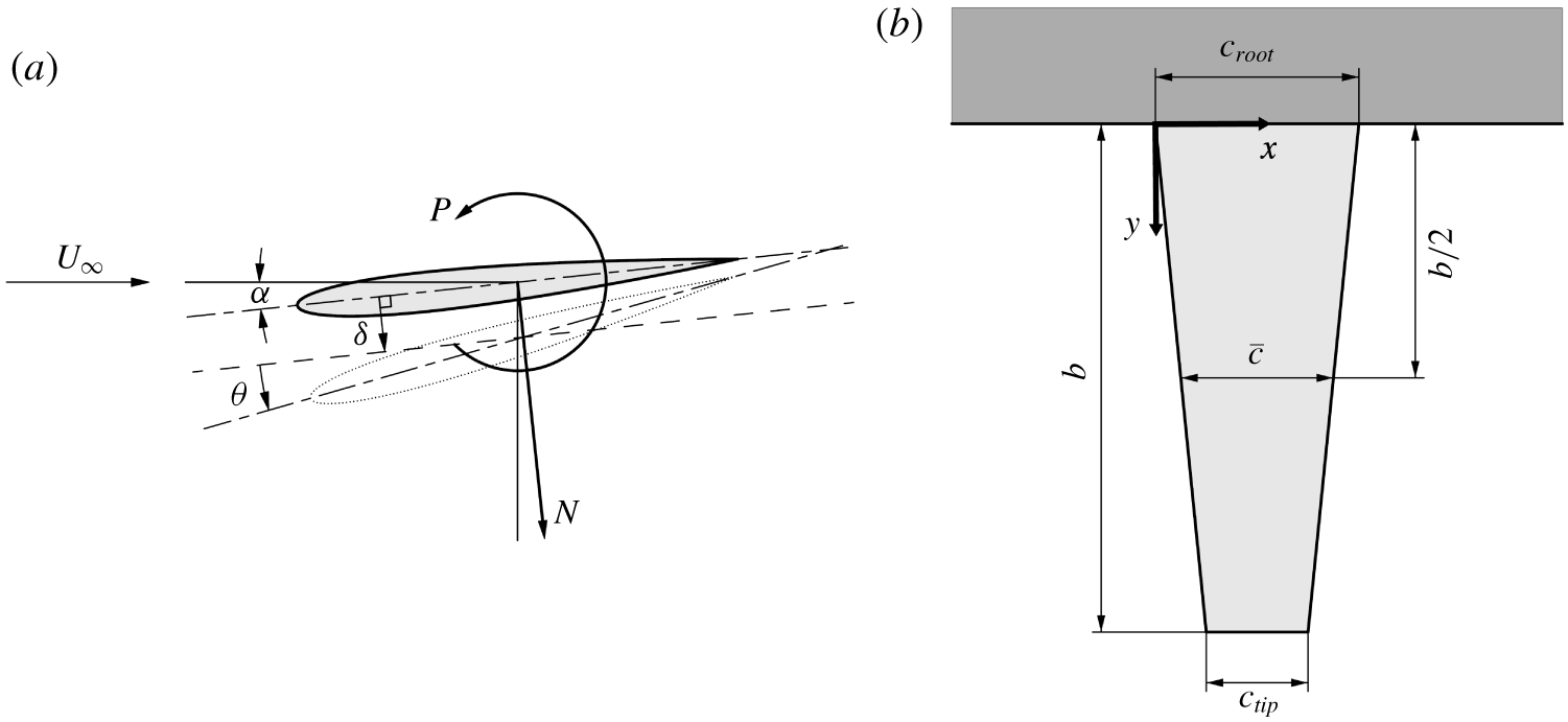
The geometric and mechanical properties of the hydrofoil have been selected based on the requirements for modelling the static and dynamic FSI typical of control surfaces and propellers. The hydrofoil features a symmetric (unswept) trapezoidal planform of 300 mm span,  $b$, with a 60 mm tip chord,
 $c_{tip}$, and
 $120$ mm root chord,
 $c_{root}$, resulting in a mean chord,
 $\bar{c}=(c_{root}+c_{tip})/2$, of
 $90$ mm. This gives an aspect ratio (
 $b/\bar{c}$) of
 $3.33$, typical of marine propellers. The model has a modified NACA0009 section profile that features a thicker trailing edge for improved robustness against trailing-edge damage and to allow for manufacturing of the compliant composite models (Zarruk et al. Reference Zarruk, Brandner, Pearce and Phillips2014). Experiments performed by Zarruk et al. (Reference Zarruk, Brandner, Pearce and Phillips2014) show that the modified profile has minimal effect on the forces and deflections experienced by the hydrofoil compared to the original NACA0009 profile. The stainless steel model was machined from a billet of Type 316 stainless steel and manufactured to a
 $\pm 0.1$ mm surface tolerance and
 $0.8~\unicode[STIX]{x03BC}\text{m}$ surface finish.
The normal force,  $N$, and pitching moment,
 $P$, acting on the hydrofoil are presented as dimensionless coefficients as
 $C_{N}=2N/\unicode[STIX]{x1D70C}U_{\infty }^{2}\bar{c}b$ and
 $C_{P}=2P/\unicode[STIX]{x1D70C}U_{\infty }^{2}\bar{c}^{2}b$, respectively, with the coordinate system presented in figure 4(a). The hydrofoil first mode is in bending as shown by Clarke et al. (Reference Clarke, Butler, Crowley and Brandner2014) and measured frequencies for various conditions and techniques are summarised in table 1. These results show the difference in frequencies for in air, fully wetted and the influence of mounting compliance. The natural frequency,
 $f_{n}$, reduces by approximately 10 % when mounted from the force balance compared with rigid mounting. Excitation of the first mode should then be expected to occur between
 $St_{n}=f_{n}\bar{c}/U_{\infty }$ values of about 0.5 and 0.9 depending on cavity extent affecting added mass as marked on figure 8.
Coordinate system used for both the forces and tip deflection of the hydrofoil (a) is located at the mid-chord along the centreline. The deformed hydrofoil tip is represented by the dotted outline where the tip bending displacement,  $\unicode[STIX]{x1D6FF}$, is measured by taking the mean displacement of the profile edge perpendicular to the centreline at the zero-load case. The tip twist deflection,
 $\unicode[STIX]{x1D703}$, is the rotation of the profile centreline from the zero-load case. A schematic of the hydrofoil’s tapered planform (b) shows the coordinate system used in the analysis of the cavitation behaviour (e.g. cavity length) is located at the leading edge of the root chord.

First mode frequencies in bending of the NACA0009 stainless steel hydrofoil for various conditions as reported by Clarke et al. (Reference Clarke, Butler, Crowley and Brandner2014). The in water (fully wetted) measurements were made using digital image correlation (DIC) and force measurements and the in air using impact/accelerometer.

2.3 Experimental techniques
To obtain detailed information of loading variations on the hydrofoil through various cavitation regimes, long-duration force measurements were made at  $\unicode[STIX]{x1D70E}$ increments of
 $0.025$. Tip deflection and cavitation behaviour measurements, discussed further below, were obtained simultaneously (including force measurements) using high-speed photography at
 $\unicode[STIX]{x1D70E}$ increments of
 $0.1$. For these simultaneous measurements, due to limitations with respect to camera memory storage, ‘medium’ length, reduced temporal resolution runs were acquired suitable for statistical analysis of the imaging data sets and ‘short’ length, high temporal resolution data sets were acquired for a detailed analysis of the cavitation physics. Details of all three run types are summarised in table 2.
The force time series were analysed using the continuous wavelet transform, following the procedure of Torrence & Compo (Reference Torrence and Compo1998). The Morlet wavelet was applied and correlated at various scales with the time series, allowing events and intermittent components in the force and tip displacement history to be identified. Time-series data are presented with time,  $t$, being non-dimensionalised as
 $t^{\prime }=tU_{\infty }/\bar{c}$.
2.3.1 Tip deflection
The tip deflection of the hydrofoil was measured via high-speed photography utilising a Phantom v2640 with a Nikkor  $105$ mm
 $f/2.8$G lens (figure 2). Operating with a resolution of
 $512\times 1504$ pixels and a spatial resolution of
 $0.049~~\text{mm}~\text{px}^{-1}$. The tip deflection was determined using edge detection of the hydrofoil tip profile and comparing each frame to the hydrofoil under zero load based on the assumption that the profile locally remains undeformed. The edge detection process involved first rotating each frame by the angle of the hydrofoil under zero load relative to the frame using bicubic interpolation and then applying a 2-D Gaussian filter to smooth the image. The edge was detected along the profile based on peaks in the pixel intensity gradient along each row. Outliers were identified as being more than three standard deviations away from the local mean within a 50 element window and replaced using linear interpolation. The difference between the loaded and unloaded case gave the tip deflection with tip bending displacement,
 $\unicode[STIX]{x1D6FF}$, taken as the average distance of every row with the twist,
 $\unicode[STIX]{x1D703}$, determined from a line of best fit through the data with the tip displacement subtracted. Positive
 $\unicode[STIX]{x1D6FF}$ is defined as translation towards the suction side with positive
 $\unicode[STIX]{x1D703}$ defined as nose up, as shown in figure 4. For the stainless steel model, no twist was clearly resolved within the precision of the method employed, indicating it is negligible, as was also reported by Zarruk et al. (Reference Zarruk, Brandner, Pearce and Phillips2014) using high-resolution still photography for static deflections.
Test matrix for the various run types detailing the  $\unicode[STIX]{x1D70E}$ range, run duration,
 $T$, high-speed photography frame rate,
 $f_{HSP}$, and force balance sampling rate,
 $f_{FB}$. The Long acquisition periods provided high-resolution loading behaviour with
 $\unicode[STIX]{x1D70E}$. Due to camera storage limitations, simultaneous force measurement and high-resolution imaging of the cavitation behaviour and tip deflections was obtained with the Medium and Short run types, respectively.

2.3.2 Cavitation behaviour
The cavitation behaviour over the suction side of the hydrofoil was recorded using a second Phantom v2640 high-speed camera with a Nikkor 50 mm  $f/1.8$D lens (figure 2). The camera was operated with a resolution of
 $2048\times 1952$ pixels and a spatial resolution of
 $0.185~\text{mm}~\text{px}^{-1}$ with the same optical arrangement used for both the medium and short run acquisition types.
To identify coherent structures in the dynamic cloud cavitation behaviour, spectral proper orthogonal decomposition (SPOD) is employed using the technique outlined by Towne, Schmidt & Colonius (Reference Towne, Schmidt and Colonius2018). In this instance the SPOD is applied to the time-varying image intensity as opposed to time-varying velocity data from time resolved particle image velocimetry as typically used. SPOD optimally represents the space–time flow statistics by identifying energy ranked modes that are dynamically significant (Schmidt et al. Reference Schmidt, Towne, Rigas, Colonius and Bres2018). Each high-speed photography acquisition provided time-varying data (with image sequence) of the spatial variation (2 dimensional) of pixel intensity. Due to light scattering from interfacial surfaces, a high intensity was recorded where there was the presence of a cavity or bubbly mixture/shed cloud. Analysing these image data sets with SPOD allowed for the identification of various shedding modes, both in frequency content and the spatial location.
SPOD utilises multiple realisations of the temporal Fourier transform of the flow field, in this case the dynamic behaviour of the cavity, to obtain convergent estimates of the spectral densities by appropriately averaging the spectra, achieved using Welch’s method (Welch Reference Welch1967) with a Hanning window. The decomposition was performed on the high-speed photography data, consisting of  $n_{x}$ rows and
 $n_{y}$ columns, obtained from the medium run types at each
 $\unicode[STIX]{x1D70E}$. The pixel intensity time series of each pixel was broken up into blocks with a length,
 $N_{f}$, of 256 snapshots, representing 0.512 s. The overlap between blocks,
 $N_{o}$, was 128 snapshots, representing 0.256 s. This results in 128 blocks,
 $N_{b}$, for the 18 000 snapshot long sequence, and producing a frequency resolution of 1.95 Hz for the extracted SPOD modes.
An overview of the SPOD calculation procedure applied to the data is given in the following with a detailed description of the SPOD methodology and algorithm given by Towne et al. (Reference Towne, Schmidt and Colonius2018). For the  $n\text{th}$ block, the matrix,
 $\unicode[STIX]{x1D64C}^{(n)}$, is built from a portion of the high-speed movie, reshaped to have as many rows as pixels,
 $N=n_{x}\times n_{y}$, and
 $N_{f}$ columns, being the number of frames in each block. Each block is structured with the
 $k\text{th}$ frame in the
 $n\text{th}$ block represented as
 $\boldsymbol{q}_{k}^{(n)}$ (2.1). These are considered to be statistically independent realisations of the flow under the ergodic hypothesis.
 $$\begin{eqnarray}\unicode[STIX]{x1D64C}^{(n)}=[\boldsymbol{q}_{1}^{(n)},\boldsymbol{q}_{2}^{(n)},\ldots ,\boldsymbol{q}_{N_{f}}^{(n)}]\in \mathbb{R}^{N\times N_{f}}.\end{eqnarray}$$
Once the data matrix is correctly structured into  $N_{b}$ blocks, the Fourier transform is calculated for the
 $n\text{th}$ block using (2.2). Each block is then structured again as shown in (2.3) with
 $\hat{\boldsymbol{q}}_{k}^{(n)}$ being the
 $n\text{th}$ realisation of the Fourier transform at the
 $k\text{th}$ discrete frequency.
 $$\begin{eqnarray}\displaystyle & \displaystyle \hat{\boldsymbol{q}}_{k}^{(n)}=\frac{1}{2N_{f}}\mathop{\sum }_{j=1}^{N_{f}}w_{j}\boldsymbol{q}_{j}^{(n)}\text{e}^{\text{i}2\unicode[STIX]{x03C0}(k-1)[(j-1)/N_{f}]}, & \displaystyle\end{eqnarray}$$
 $$\begin{eqnarray}\displaystyle & \displaystyle \hat{\unicode[STIX]{x1D64C}}^{(n)}=[\hat{\boldsymbol{q}}_{1}^{(n)},\hat{\boldsymbol{q}}_{2}^{(n)},\ldots ,\hat{\boldsymbol{q}}_{N_{f}}^{(n)}]. & \displaystyle\end{eqnarray}$$
The scalar weights,  $w_{j}$, are nodal values of the Hanning window function that can be used to reduce spectral leakage due to non-periodicity of the data in each block.
For each frequency,  $k$, the Fourier coefficients of each block are collected into the new matrix
 $\hat{\unicode[STIX]{x1D64C}}_{f_{k}}$, as shown in (2.4).
 $$\begin{eqnarray}\hat{\unicode[STIX]{x1D64C}}_{f_{k}}=[\hat{\boldsymbol{q}}_{k}^{(1)},\hat{\boldsymbol{q}}_{k}^{(2)},\ldots ,\hat{\boldsymbol{q}}_{k}^{(N_{b})}]\in \mathbb{R}^{N\times N_{b}}.\end{eqnarray}$$
This allows the weighted cross spectral density tensor,  $\unicode[STIX]{x1D64E}_{f_{k}}$, at frequency
 $f_{k}$ to be written as (2.5) where
 $(\cdot )^{\ast }$ denotes the Hermitian transpose.
 $$\begin{eqnarray}\unicode[STIX]{x1D64E}_{f_{k}}=\hat{\unicode[STIX]{x1D64C}}_{f_{k}}\hat{\unicode[STIX]{x1D64C}}_{f_{k}}^{\ast }.\end{eqnarray}$$
From  $\unicode[STIX]{x1D64E}_{f_{k}}$, the SPOD modes of the
 $k\text{th}$ frequency,
 $\unicode[STIX]{x1D731}_{f_{k}}$, can be found as the eigenvectors from (2.6).
 $$\begin{eqnarray}\unicode[STIX]{x1D64E}_{f_{k}}\unicode[STIX]{x1D652}\unicode[STIX]{x1D731}_{f_{k}}=\unicode[STIX]{x1D731}_{f_{k}}\unicode[STIX]{x1D726}_{f_{k}},\end{eqnarray}$$
where  $\unicode[STIX]{x1D652}$ is a positive–definite Hermitian matrix that accounts for both the weight
 $\unicode[STIX]{x1D652}(x)$ and the numerical quadrature of the integral of the discrete grid.
However, solving this is computationally expensive and it has been shown by Towne et al. (Reference Towne, Schmidt and Colonius2018) that the modes can be recovered by solving the  $N_{b}\times N_{b}$ eigenvalue problem in (2.7).
 $$\begin{eqnarray}\hat{\unicode[STIX]{x1D64C}}_{f_{k}}^{\ast }\unicode[STIX]{x1D652}\hat{\unicode[STIX]{x1D64C}}_{f_{k}}\unicode[STIX]{x1D723}_{f_{k}}=\unicode[STIX]{x1D723}_{f_{k}}\tilde{\unicode[STIX]{x1D726}}_{f_{k}}.\end{eqnarray}$$
The non-zero eigenvalues of (2.6) are recovered and indicated by  $\tilde{(\cdot )}$. By projecting the Fourier coefficients,
 $\hat{\unicode[STIX]{x1D64C}}_{f_{k}}$, onto the new eigenvectors,
 $\unicode[STIX]{x1D723}_{f_{k}}$, as shown in (2.8), the mode shapes are obtained exactly.
 $$\begin{eqnarray}\tilde{\unicode[STIX]{x1D731}}_{f_{k}}=\hat{\unicode[STIX]{x1D64C}}_{f_{k}}\unicode[STIX]{x1D723}_{f_{k}}\tilde{\unicode[STIX]{x1D726}}_{f_{k}}^{-1/2}.\end{eqnarray}$$
The modes ( $\tilde{\unicode[STIX]{x1D731}}_{f_{k}}$) are ranked in order of intensity by their eigenvalues in (2.9). As shown in Venning et al. (Reference Venning, Giosio, Pearce and Brandner2018a), the first mode of each frequency,
 $\unicode[STIX]{x1D719}_{f_{k}}^{(1)}$, is the most indicative of the ‘mean’ flow state and as such will be the only modes presented throughout the paper.
 $$\begin{eqnarray}\tilde{\unicode[STIX]{x1D731}}_{f_{k}}=[\unicode[STIX]{x1D719}_{f_{k}}^{(1)},\unicode[STIX]{x1D719}_{f_{k}}^{(2)},\ldots ,\unicode[STIX]{x1D719}_{f_{k}}^{(N_{b})}].\end{eqnarray}$$
This information gives insight into the excitation spectrum induced by the cloud cavitation and can be compared to the response spectrum to aid in identifying certain components such as cloud cavitation-induced force fluctuations and structural natural frequencies. Intensity maps are generated through colour-scaled plots where the intensity level of each pixel is proportional to the intensity level of the corresponding frequency. This provides spatial information revealing the distribution across the image of the shedding modes. By plotting the phase of the Fourier coefficients across the domain, insight into shedding cycle behaviour and interaction between events across the hydrofoil may be gained.
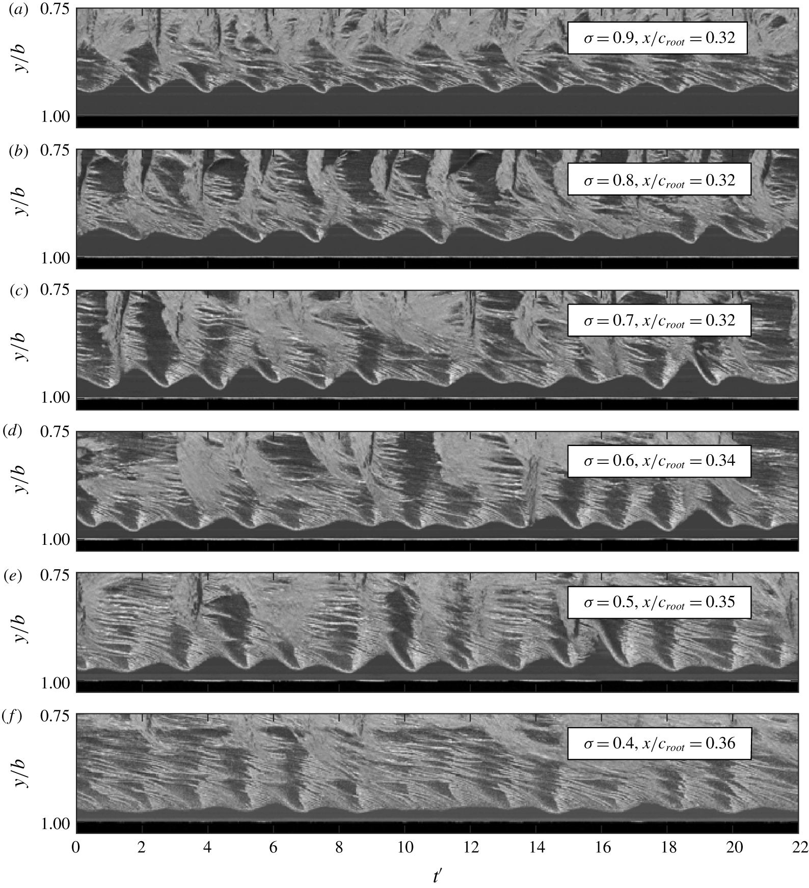
Spatio-temporal information of the cavitation behaviour is also represented through the use of space–time plots. These plots are generated by extracting either the same row or column of pixels from each frame and placing them sequentially next to one another, producing chordwise and spanwise space–time plots, respectively. Interpretation of these plots are discussed in detail by Smith et al. (Reference Smith, Venning, Giosio, Brandner, Pearce and Young2019).
3 Results and discussion
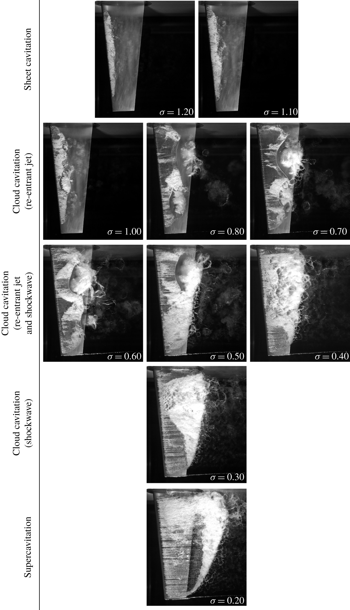
As  $\unicode[STIX]{x1D70E}$ is progressively reduced beyond inception the hydrofoil experiences various forms of cavitation. The extent of the cavitation varies from short partial sheet cavities to supercavitation (Franc & Michel Reference Franc and Michel2004). The characteristics of each regime vary in appearance and an overview of the various regimes is presented in figure 5. Traits are observed to not only vary between each of the cavitation regimes, but also within the regimes themselves. Characterising the cavitating behaviour and the corresponding influence on the hydrofoil’s performance is achieved by establishing correlations between the measured forces and deflections with the cavitation behaviour observed in the high-speed photography. For the
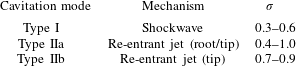
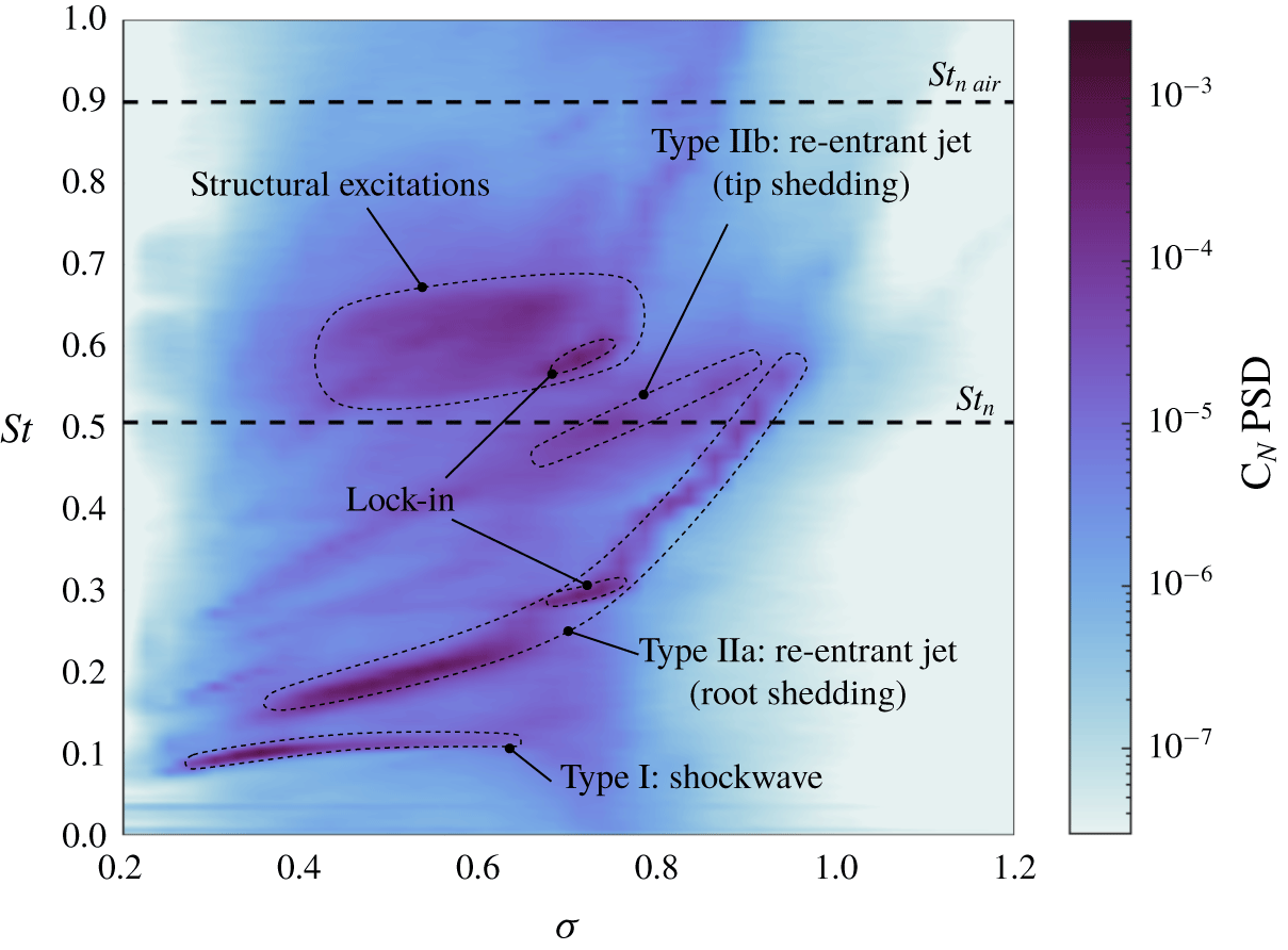
 $\unicode[STIX]{x1D70E}$ range tested, three primary cavitation modes experienced by the hydrofoil were identified which varied in both the mechanism driving shedding as well as the location on the hydrofoil. These cavitation modes are summarised in table 3 as well as indicated in the spectrograms in figure 8.
Photographs of the hydrofoil with different cavitation regimes through the range of  $\unicode[STIX]{x1D70E}$ below inception. The hydrofoil first experiences stable sheet cavitation (
 $1.1\leqslant \unicode[STIX]{x1D70E}<1.2$), with development of re-entrant jet-driven cloud cavitation as
 $\unicode[STIX]{x1D70E}$ is reduced (
 $0.4\leqslant \unicode[STIX]{x1D70E}\leqslant 1.0$). With a further reduction in
 $\unicode[STIX]{x1D70E}$, with cavity length extending to the trailing edge, upstream propagating condensation shockwaves become the dominant mechanism for shedding (
 $0.3\leqslant \unicode[STIX]{x1D70E}<0.4$). For
 $\unicode[STIX]{x1D70E}<0.3$, the cavity envelopes the hydrofoil (supercavitation) and the break-up region is downstream of the trailing-edge.

Summary of the cavitation modes experienced by the hydrofoil for the  $\unicode[STIX]{x1D70E}$ range tested. As
 $\unicode[STIX]{x1D70E}$ is reduced from 1.2, the hydrofoil first starts experiencing the re-entrant-driven Type IIa mode at
 $\unicode[STIX]{x1D70E}=1.0$ with the Type IIb becoming active shortly after at
 $\unicode[STIX]{x1D70E}=0.9$. Further reduction in
 $\unicode[STIX]{x1D70E}$ sees the disappearance of the Type IIb mode below 0.7 with the shockwave-driven Type I mode becoming active at
 $\unicode[STIX]{x1D70E}=0.6$. The Type IIa mode remains active along with the Type I mode down to
 $\unicode[STIX]{x1D70E}=0.4$ before disappearing, resulting solely shockwave-driven shedding at
 $\unicode[STIX]{x1D70E}=0.3$. Supercavitation is reached at
 $\unicode[STIX]{x1D70E}=0.2$ where no cavitation modes are active.

3.1 Cavity length
The length of the attached cavity was measured for each  $\unicode[STIX]{x1D70E}$ with the cavity length,
 $L_{c}$, taken as the furthest downstream extent of the cavity while remaining attached. When shedding is present, this is the cavity extent in each cycle prior to the shedding event. Cavity lengths were obtained at 4 spanwise positions from chordwise space–time diagrams extracted from the long-duration videos as an average from at least 50 cavity growth/shedding cycles.
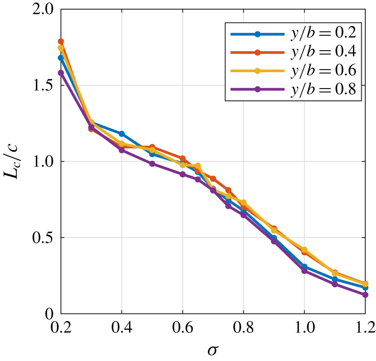
The presence and extent of an attached cavity influences the pressure distribution over the hydrofoil and therefore the forces that result. In cloud cavitation conditions, the attached part of the cavity limits the minimum pressure on the suction side to the vapour pressure of the water (Franc Reference Franc2001). Figure 6 shows the maximum attached cavity length,  $L_{c}$ normalised by the local chord,
 $c$, as a function of
 $\unicode[STIX]{x1D70E}$ and spanwise position. For
 $0.4\leqslant \unicode[STIX]{x1D70E}\leqslant 0.6$, the cavity length exhibits a reduction in the rate of increase with reducing
 $\unicode[STIX]{x1D70E}$ compared to higher
 $\unicode[STIX]{x1D70E}$ ranges. This reduction in cavity-length growth rate corresponds to the attached cavity reaching the trailing edge, i.e.
 $L_{c}/c=1.0$. At this stage of development the cavity closure will now directly interact with the flow from the pressure side of the foil, possibly causing the rate of growth to reduce. When
 $\unicode[STIX]{x1D70E}$ is reduced to 0.2 the cavity length increases to well beyond the local chord, indicating the cavity closure is away from the trailing edge and hence is in the super-cavitating regime.
Maximum attached cavity length,  $L_{c}$, as a function of
 $\unicode[STIX]{x1D70E}$, for four spanwise positions. The cavity length is the average length at cavity break-off, and is non-dimensionalised by the local chord,
 $c$, at each position. The cavity growth is continuous as
 $\unicode[STIX]{x1D70E}$ is reduced.

3.2 Steady and unsteady components of the forces and deflections
The mean and standard deviation of the normal force ( $C_{N}$) and pitching moment (
 $C_{P}$) provide insight into the impact of the cavitation on the hydrofoil in terms of both the steady and unsteady forces. Spatial information is obtained through the centre of pressure,
 $x_{cop}$, which gives the centre of action of the forces acting along the hydrofoil and is calculated as
 $C_{P}/C_{N}$ and presented as a ratio of the mean chord,
 $x_{cop}/\bar{c}$, from the leading edge at the root. The non-dimensional tip displacement,
 $\unicode[STIX]{x1D6FF}/\bar{c}$, is presented to assess the level of structural response resulting from the hydrodynamic loading.
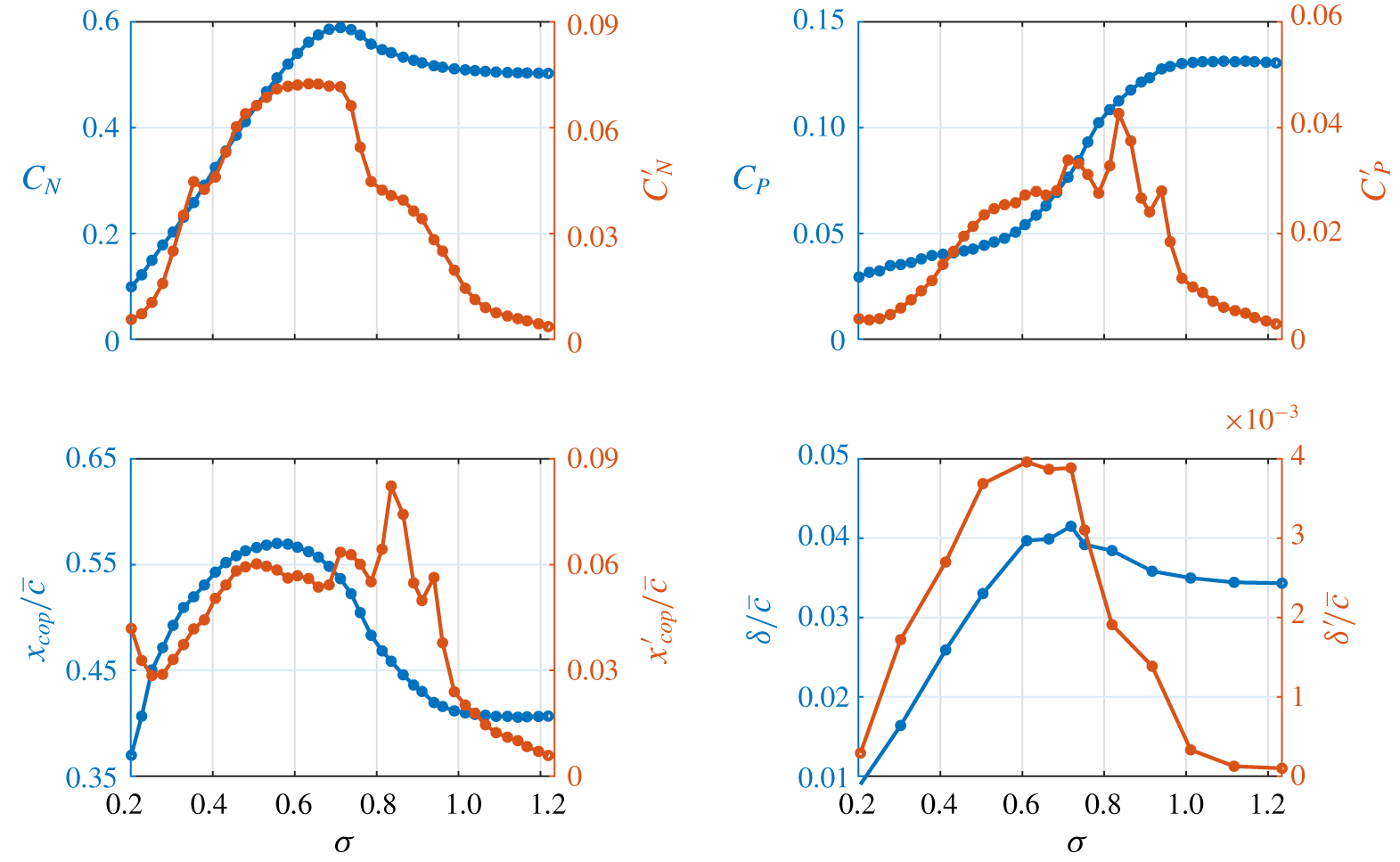
The mean and standard deviation of  $C_{N}$,
 $C_{P}$,
 $x_{cop}/\bar{c}$ and
 $\unicode[STIX]{x1D6FF}/\bar{c}$ are shown in figure 7 as functions of
 $\unicode[STIX]{x1D70E}$, with
 $^{\prime }$ denoting the standard deviation of the time-varying quantities. As
 $\unicode[STIX]{x1D70E}$ is decreased from 1.2 to 1.1 (sheet cavitation regime, see figure 5), all standard deviations increase despite little change in the mean load and displacement. Further reduction in
 $\unicode[STIX]{x1D70E}$ to 1.0 sees a significant change in the unsteady loading with
 $C_{N}^{\prime }$ approximately doubling and is attributed to the transition to the cloud cavitation regime with re-entrant jet-driven shedding at
 $\unicode[STIX]{x1D70E}\approx 1.0$. This increased unsteadiness is attributed to the increased volume of the shedding clouds associated with re-entrant jet-driven shedding compared to sheet cavitation having greater impact on the hydrofoil’s pressure distribution.
Initially as  $\unicode[STIX]{x1D70E}$ is reduced into the cloud cavitation regime (
 $0.3\leqslant \unicode[STIX]{x1D70E}\leqslant 1.0$),
 $C_{N}$ continues to increase, reaching a maximum at
 $\unicode[STIX]{x1D70E}=0.71$, corresponding with the maxima in
 $C_{N}^{\prime }$,
 $\unicode[STIX]{x1D6FF}/\bar{c}$ and
 $\unicode[STIX]{x1D6FF}^{\prime }/\bar{c}$. This is attributed to the increase in effective camber of the cavitating hydrofoil due to the presence of the cavity and is discussed further in § 3.4.2. There is a marked increase in
 $C_{N}^{\prime }$ and
 $\unicode[STIX]{x1D6FF}^{\prime }/\bar{c}$ for
 $\unicode[STIX]{x1D70E}=0.8$ to
 $0.7$ which is associated with the lock-in phenomenon discussed later in § 3.4.3. Further reduction in
 $\unicode[STIX]{x1D70E}$ below 0.7 sees a steady decrease in
 $C_{N}$ and
 $C_{N}^{\prime }$ with the mean normal force reducing monotonically into the super-cavitating regime.
Despite  $C_{N}$ initially increasing with reducing
 $\unicode[STIX]{x1D70E}$,
 $C_{P}$ decreases with the onset of unsteady shedding, dropping more sharply as
 $\unicode[STIX]{x1D70E}$ is reduced from
 $1.0$ to
 $0.7$. This is due to the growing cavity shifting the
 $x_{cop}$ towards mid-chord, reducing the lever arm of the applied load. The rate
 $C_{P}$ decreases is reduced as the cavity approaches the trailing edge at
 $\unicode[STIX]{x1D70E}\approx 0.6$ with
 $x_{cop}/\bar{c}$ reaching a maximum of
 $0.57$ at
 $\unicode[STIX]{x1D70E}=0.56$. Interestingly,
 $x_{cop}$ starts moving back towards the leading edge as
 $\unicode[STIX]{x1D70E}$ drops further despite the cavity covering the entire chord as the pressure field varies around the combined hydrofoil/growing cavity system. The displacement and normal force measurements, both mean and standard deviation, exhibit similar trends, indicating a strong correlation between the two as expected. A strong correlation is also observed between
 $x_{cop}^{\prime }$ and
 $C_{P}^{\prime }$.
Mean (blue) and standard deviation (orange) of the normal force ( $C_{N}$), pitching moment (
 $C_{P}$), location of the centre of pressure (
 $x_{cop}/\bar{c}$) and tip displacement (
 $\unicode[STIX]{x1D6FF}/\bar{c}$) at various
 $\unicode[STIX]{x1D70E}$ where
 $^{\prime }$ indicates the standard deviation of the time-varying quantity. The results show the effect of various cavitation regimes revealing unique characteristics in the steady and unsteady components.

3.3 Force and deflection spectra
The amplitude and frequency content of the forces acting on the hydrofoil is dependent on multiple factors including hydrodynamic loading, cavitation dynamics and the structural response. A spectrogram of  $C_{N}$ for varying
 $\unicode[STIX]{x1D70E}$ (figure 8) provides a global perspective of how the cavitation behaviour modulates the spectral characteristics. The spectrogram is constructed from spectra of the long-duration measurements at
 $0.025$ increments of
 $\unicode[STIX]{x1D70E}$. Spectra of
 $C_{N}$ were obtained using the power spectral density (PSD) derived with the Welch estimate (Welch Reference Welch1967) utilising a Hanning window with size and overlap of 2048 (2.05 s) and 512 (0.51 s) samples, respectively, on the 360 000 (360 s) sample time series. Frequency is non-dimensionalised as a chord-based Strouhal number,
 $St=fc/U_{\infty }$. Individual spectrum plots at
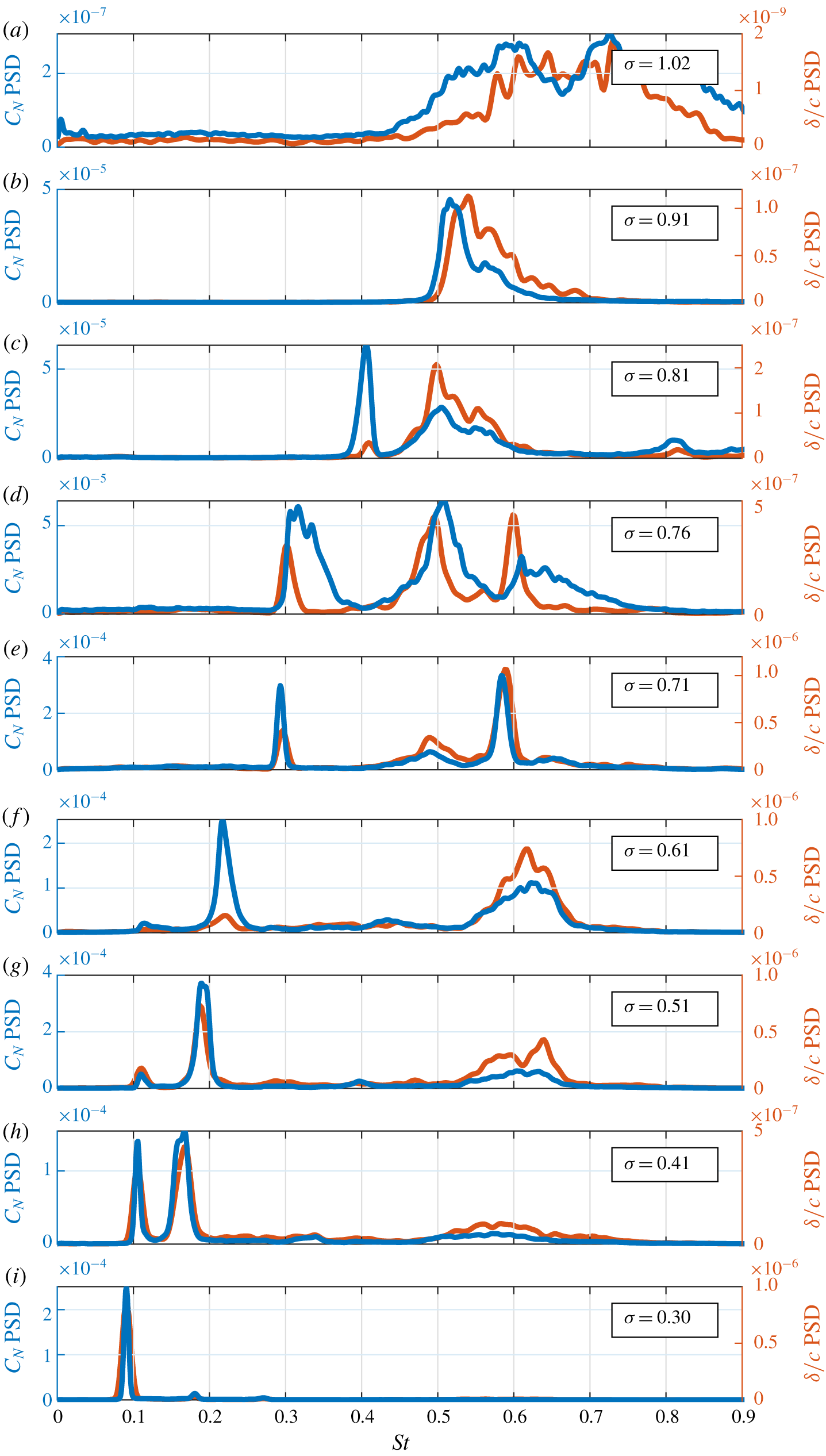
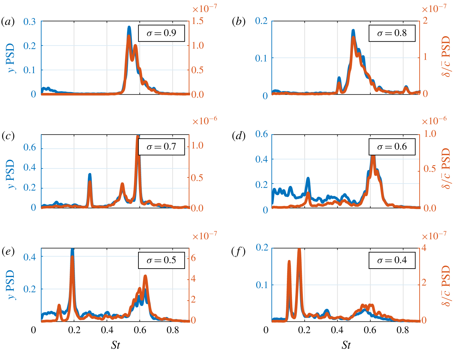
 $\unicode[STIX]{x1D70E}$ values of particular interest are presented in figure 9 along with the corresponding tip deflection spectra calculated from the medium duration time-series data.
Spectrogram of the normal force for a range of  $\unicode[STIX]{x1D70E}$ showing the global unsteady behaviour. The results highlight the shockwave-driven Type I shedding frequency is predominantly independent of
 $\unicode[STIX]{x1D70E}$ while the re-entrant jet-driven Type IIa and IIb shedding modes are highly dependent on
 $\unicode[STIX]{x1D70E}$. The natural frequency of the hydrofoil in air,
 $St_{n\hspace{2.22198pt}air}$, and fully wetted,
 $St_{n}$, are indicated by two horizontal dashed lines.

PSD of the normal force (blue) and tip displacement (orange) time series at selected  $\unicode[STIX]{x1D70E}$. The various spectra show the peak frequencies shift as
 $\unicode[STIX]{x1D70E}$ varies with both the normal force and tip displacement exhibiting similar spectral characteristics across the selected
 $\unicode[STIX]{x1D70E}$ values. Note that the vertical scales vary (by orders of magnitude) between the plots.

There are 3 primary modes identified in the spectra which are referred to as Types I, IIa and IIb in the text. The Type I mode is associated with shockwave-driven periodic shedding occurring along a majority of the span with the shedding frequency observed to be essentially independent of  $\unicode[STIX]{x1D70E}$. The Type IIa and IIb modes are both driven by a re-entrant jet instability and are dependant on
 $\unicode[STIX]{x1D70E}$. Type IIa ‘root shedding’ events occur at various spanwise positions depending on
 $\unicode[STIX]{x1D70E}$, while Type IIb ‘tip shedding’ events are confined to the lower portion (
 $0.5<y/b<1.0$). This nomenclature follows that used by Kjeldsen & Arndt (Reference Kjeldsen and Arndt2001) where shockwave and re-entrant jet type shedding mechanisms were termed Types I and II, respectively. The analysis undertaken to identify these various modes is described in § 3.4.
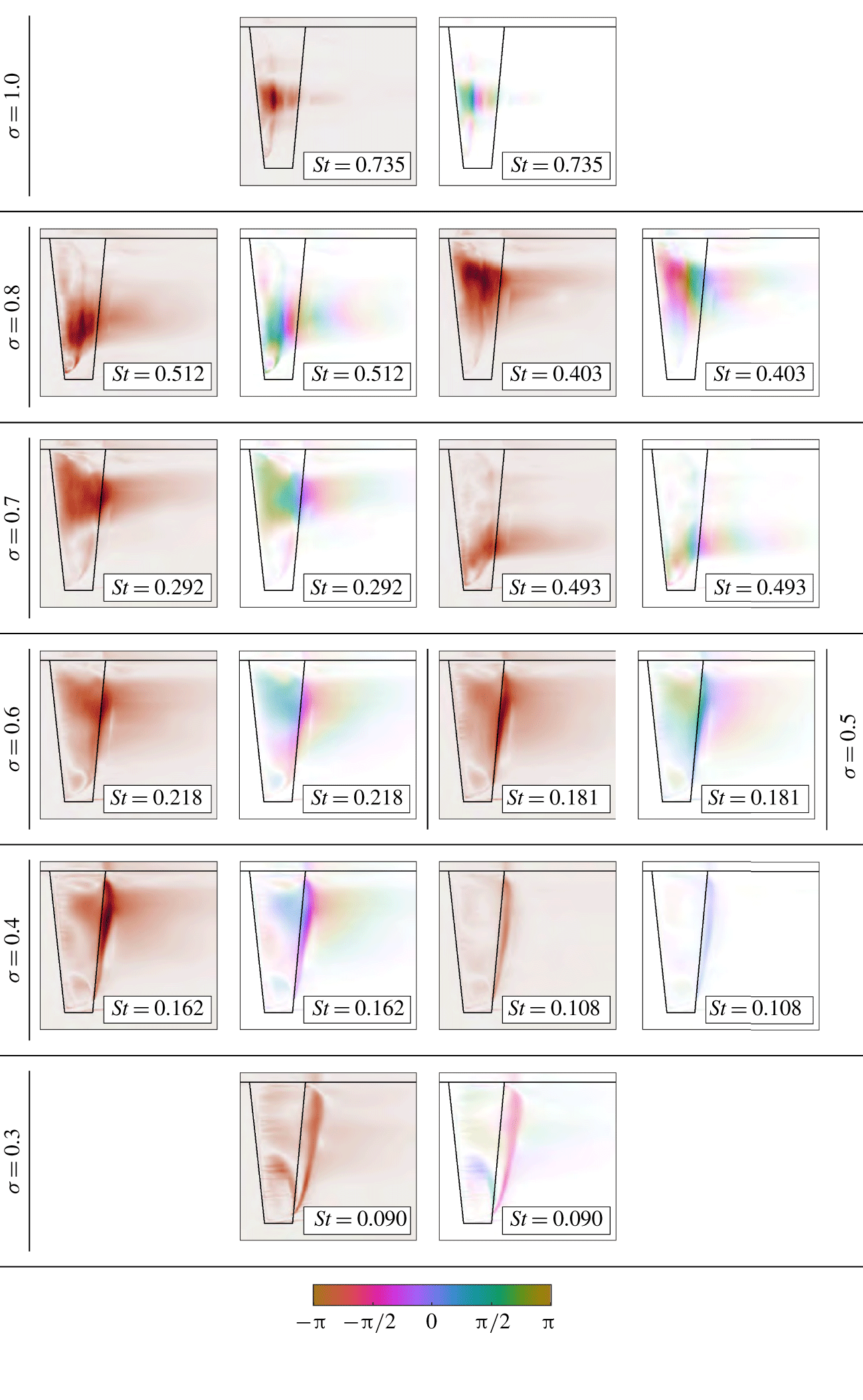
As previously observed with both 2-D (Kawanami et al. Reference Kawanami, Kato and Yamaguchi1998; Prothin et al. Reference Prothin, Billard and Djeridi2016) and 3-D geometries (Smith et al. Reference Smith, Venning, Brandner, Pearce, Giosio and Young2018), the cavitation pattern over a hydrofoil varies with  $\unicode[STIX]{x1D70E}$, such as shedding sites, cavity length and cavitation cloud size. The frequency at which these shedding events occur is also dependant on their spanwise location, particularly in the present case of finite and spanwise-varying geometry. Utilising the intensity maps from the SPOD (figure 10) applied to the high-speed photography provides spatial information with respect to the cloud cavitation regime to qualitatively identify periodic shedding sites at each
 $\unicode[STIX]{x1D70E}$. Used in conjunction with the
 $C_{N}$ and
 $\unicode[STIX]{x1D6FF}/\bar{c}$ response spectra, the intensity and phase maps allow modes evident in the response spectra to be attributed to associated cavity dynamics.
Spectral POD intensity (red) and phase maps (coloured) of key modes for various  $\unicode[STIX]{x1D70E}$ highlighting regions of high activity at the frequencies of interest. The colour intensity distribution in each phase map is directly proportional to that of the corresponding intensity map. The spectral and spatial information aids in the identification of the mechanisms driving oscillations with phase maps providing the relative timing of each cycle.

Within the stable sheet cavitation regime ( $\unicode[STIX]{x1D70E}\geqslant 1.1$), there is little unsteady content in
 $C_{N}$ with no tonal peaks observed in the spectrum (not shown in figure 9). Once
 $\unicode[STIX]{x1D70E}$ is reduced below
 $1.1$, with cloud cavitation forming, fluctuations in both
 $C_{N}$ and
 $\unicode[STIX]{x1D6FF}/\bar{c}$ are now significant (increasing by two orders of magnitude between
 $\unicode[STIX]{x1D70E}=1.02$ and 0.91) with distinct tonal peaks becoming apparent (figure 9b). Two distinct peaks are evident in the
 $C_{N}$ and
 $\unicode[STIX]{x1D6FF}/\bar{c}$ spectra at
 $\unicode[STIX]{x1D70E}=0.91$, both of which decrease in frequency as
 $\unicode[STIX]{x1D70E}$ is reduced to
 $0.81$ (figure 9b,c). These peaks are associated with the formation of two shedding sites along the span of the hydrofoil discussed later in § 3.4.2. The shedding at these two sites are referred to as Type IIa and Type IIb oscillations for the root and the tip, respectively.
A shift in the peak frequency occurs in conjunction with the appearance of a third peak in the spectra at  $\unicode[STIX]{x1D70E}=0.76$ as
 $\unicode[STIX]{x1D70E}$ is reduced below 0.8 (figure 9d). The
 $C_{N}$ spectrogram (figure 8) shows the Type IIa frequency jumping down to
 $St=0.31$ and increasing in magnitude with an intense peak appearing at double the frequency (
 $St=0.61$) for
 $0.7\leqslant \unicode[STIX]{x1D70E}\leqslant 0.76$. This feature is attributed to lock-in, where the Type IIa shedding frequency has transitioned to match a sub-harmonic of the hydrofoil first bending mode (
 $f_{n}$). As given in table 1, the hydrofoil first bending mode occurs at
 $55$ Hz (
 $St_{n}=0.52$) in fully wetted conditions, which is lower than the third peak at
 $St=0.61$. This difference in frequency is attributed to the presence of the vapour cavity reducing the added mass and causing frequency modulation. The Type IIb peak continues a steady decrease to
 $St=0.51$ at
 $\unicode[STIX]{x1D70E}=0.76$ (figure 9d).
Lock-in is also apparent in the tip displacement spectrum at  $\unicode[STIX]{x1D70E}=0.7$ (figure 9e) in the appearance of the third peak along with amplification of the Type IIa spectral peak (also reflected in the increase in
 $\unicode[STIX]{x1D6FF}^{\prime }/c$ shown in figure 7). As
 $\unicode[STIX]{x1D70E}$ is reduced below
 $0.65$, the hydrofoil comes out of lock-in with the Type IIa oscillations dropping to
 $St=0.22$, the Type IIb mode fading out and significant broadband excitation in
 $C_{N}$ and
 $\unicode[STIX]{x1D6FF}/\bar{c}$ appearing at
 $St\approx 0.62$ (see figure 9f) attributed to structural excitations.
The Type IIa shedding frequency continues to steadily decrease as the attached cavity length grows, showing a non-linear dependence on  $\unicode[STIX]{x1D70E}$ until it disappears at
 $\unicode[STIX]{x1D70E}\approx 0.4$. The spectra also show the emergence of an additional frequency at
 $St=0.11$ for
 $\unicode[STIX]{x1D70E}\lessapprox 0.6$ that is nominally independent of
 $\unicode[STIX]{x1D70E}$. The appearance of this new feature coincides with the cavity reaching the trailing edge (figure 6) and is attributable to the presence of the shockwave instability (Type I). In addition, the broadband excitation appearing at
 $St\approx 0.62$ is linked to structural excitations outside of lock-in conditions, apparent down to
 $\unicode[STIX]{x1D70E}=0.4$. Type I and IIa instabilities are both present from
 $\unicode[STIX]{x1D70E}=0.6$ down to 0.4 with the Type I amplitude increasing as
 $\unicode[STIX]{x1D70E}$ is reduced.
Once  $\unicode[STIX]{x1D70E}$ is reduced below
 $0.4$, only the Type I mode remains with
 $St\approx 0.09$ oscillations dominant, as shown in figure 9(i). As also observed by Kjeldsen et al. (Reference Kjeldsen, Arndt and Effertz2000) and Smith et al. (Reference Smith, Venning, Brandner, Pearce, Giosio and Young2018), the Type I mode shows little to no dependence on
 $\unicode[STIX]{x1D70E}$, however, Kawakami et al. (Reference Kawakami, Fuji, Tsujimoto and Arndt2008) found this only to be valid for cases with relatively high gas content (
 ${\sim}13$ ppm), which was not the condition in the present study.
The shockwave-driven Type I mode is no longer apparent in the super-cavitating regime ( $\unicode[STIX]{x1D70E}=0.2$). The
 $C_{N}$ spectrogram (figure 8) reveals minimal excitations with no tonal peaks for
 $\unicode[STIX]{x1D70E}=0.2$. All associated cavity dynamics with observations made in the forces and deflections for each cavitation regime will be discussed in § 3.4.
3.4 Cavity dynamics
3.4.1 Sheet cavitation
Sheet cavitation occurs at relatively high  $\unicode[STIX]{x1D70E}$ (
 $1.1\leqslant \unicode[STIX]{x1D70E}\leqslant 1.2$) and is confined to a small portion of the chord towards the leading edge (supplementary movie 1, available at https://doi.org/10.1017/jfm.2020.321). The space–time plot taken at
 $x/c_{root}=0.35$ (figure 11) shows coherent shedding of small-scale vapour structures. However, the cavity at the extreme extents (not shown in the space–time plot) is stabilised by the re-entrant jet at the tip and the tunnel ceiling boundary layer at the root. Cavity break-up is driven primarily by interfacial instabilities such as Kelvin–Helmholtz-driven spanwise vorticity lines (Avellan et al. Reference Avellan, Dupont and Ryhming1988) and turbulent transition (Brennen Reference Brennen1995). Some recent investigations have observed this phenomenon in cavitating flows about a rectangular planform finite-span hydrofoil (Russell et al. Reference Russell, Venning, Brandner, Pearce, Giosio and Ceccio2018) and about a sphere (Brandner et al. Reference Brandner, Walker, Niekamp and Anderson2010; de Graaf et al. Reference de Graaf, Brandner and Pearce2017). The shedding of these small-scale structures only causes minimal broadband force fluctuations as they are not large enough to cause any significant changes in the flow over the hydrofoil and, hence, unsteadiness in the pressure distribution and resulting developed forces.
Spanwise space–time plot taken at  $x/c_{root}=0.35$ shows the shedding small-scale vapour structures along the span due interfacial instabilities for
 $\unicode[STIX]{x1D70E}=1.1$. While there is evidence of periodic break-up, the influence on the forces and deflections are minimal.

As  $\unicode[STIX]{x1D70E}$ is reduced, the cavity grows into a region of an increasingly adverse pressure gradient, a re-entrant jet begins to form extending upstream along the hydrofoil surface. For the re-entrant jet to act as a mechanism for cavity break-up and cloud shedding it needs to reach the upstream extent of the cavity (Pelz, Keil & Groß Reference Pelz, Keil and Groß2017). This will only occur in practice if the cavity is sufficiently thick (Franc Reference Franc2001). Note that for a given flow configuration the cavity thickness will increase in proportion to the length. As observed by Callenaere et al. (Reference Callenaere, Franc, Michel and Riondet2001), a relatively thin cavity is highly susceptible to the interfacial instabilities of both interfaces (i.e. re-entrant jet/cavity surface) interacting, leading to break-up of the cavity into small-scale vapour structures, rather than the re-entrant jet progressing sufficiently upstream to act as a mechanism for the cloud instability. As shown in figure 5, the conditions to satisfy these requirements for cloud shedding to form are reached by
 $\unicode[STIX]{x1D70E}=1.0$.
3.4.2 Re-entrant jet-driven shedding (pre-lock-in)
Cloud cavitation occurs when  $\unicode[STIX]{x1D70E}$ is reduced to
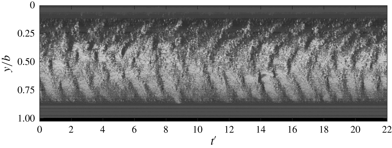
 $1.0$ with the conditions allowing the re-entrant jet to reach the upstream extent of the attached cavity, causing periodic detachment and the formation of a cavitation cloud. As shown by the space–time plot in figure 12 (supplementary movie 2), re-entrant jet-driven shedding only occurs around mid-span with the detachment of small bubbly vortices occurring towards the spanwise extents. This behaviour is also evident in the intensity maps for
 $\unicode[STIX]{x1D70E}=1.0$ at
 $St=0.74$ (figure 10). This is due to the three-dimensionality of the geometry with localised tip flow introducing a spanwise velocity component that locally prevents the re-entrant jet reaching the leading edge.
Likewise, the ceiling boundary layer modifies the local pressure distribution and streamwise velocity component in the vicinity of the root, adversely affecting formation of the re-entrant jet in the region. This results in areas of stable cavities at the spanwise extents of the attached cavity, as seen in figure 5. The shedding of cavitation clouds at  $\unicode[STIX]{x1D70E}=1.0$ induces relatively low force fluctuations, as indicated by
 $C_{N}^{\prime }$ (figure 7), at a frequency around
 $St\approx 0.70$ (evident also in the
 $C_{N}$ spectrum (figure 9) and space–time plot (figure 12)). The shedding frequency is relatively broadband and can be attributed to the varying spanwise shedding location seen in the space–time plot, where the varying cavity length changes the duration for the re-entrant jet to reach the leading edge, thus broadening the shedding frequencies present in the spectra. It is also apparent that the changing shedding location does not move randomly, but is dependent on the previous cycle. This is due to the spanwise component of the previous cycle’s re-entrant jet preventing other instabilities from interfering in the next shedding cycle at that spanwise location (de Lange & de Bruin Reference de Lange and de Bruin1998).
Spanwise space–time plot taken at  $x/c_{root}=0.31$ for
 $\unicode[STIX]{x1D70E}=1.0$ shows the re-entrant jet instability around mid-span causing periodic shedding with its spatial distribution varying through time.

As  $\unicode[STIX]{x1D70E}$ is decreased further to
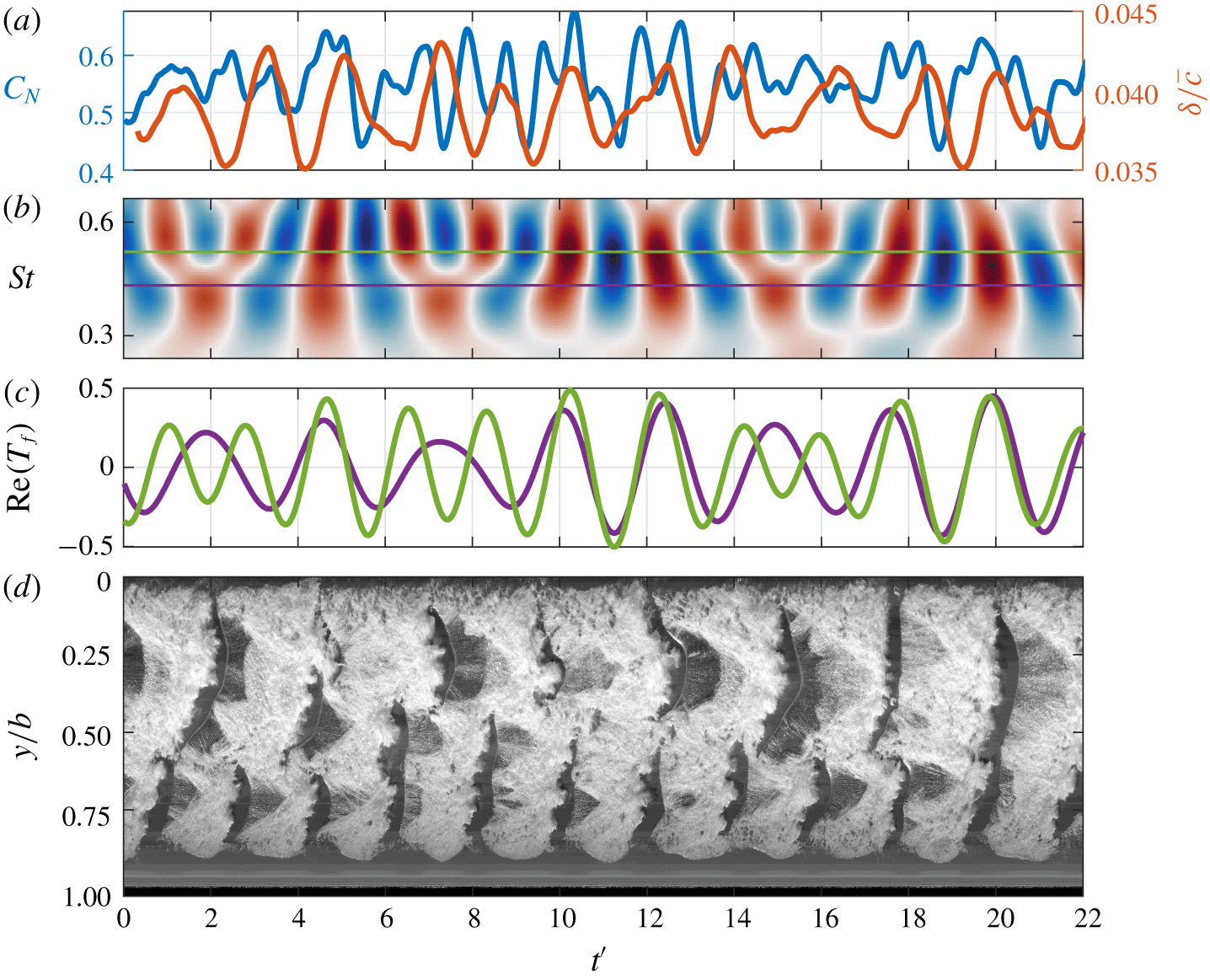
 $0.9$, the cavity size increases along with the re-entrant jet thickness (Callenaere et al. Reference Callenaere, Franc, Michel and Riondet2001), giving it the momentum to overcome spanwise flow components and reach the leading edge for the majority of the span. The increased cavity length and inherent cavity dynamics result in a spatial compatibility with the span, resulting in the formation of two re-entrant driven shedding modes (Types IIa and IIb). The increased cavity size results in significant excitation in
 $C_{N}$ and
 $\unicode[STIX]{x1D6FF}/\bar{c}$. By
 $\unicode[STIX]{x1D70E}=0.8$ two tonal frequencies become evident in the spectra (figure 9) at
 $St=0.41$ and
 $0.50$, corresponding to multiple shedding sites along the span (figure 10). As noted previously, the frequency of these modes decreases with
 $\unicode[STIX]{x1D70E}$ which is due to the re-entrant jet requiring more time to break through the attached cavity as it has more distance to travel upstream (as cavity length grows) with decreasing
 $\unicode[STIX]{x1D70E}$ (figure 6).
Synchronised time series of the normal force ( $C_{N}$) and the tip displacement (
 $\unicode[STIX]{x1D6FF}/\bar{c}$) (a) at
 $\unicode[STIX]{x1D70E}=0.8$ with the real value of the
 $C_{N}$ Morlet wavelet transform (b). The
 $St=0.41$ (purple) and
 $0.50$ (green) components of the wavelet transform (c) show the connection between the
 $C_{N}$ fluctuations and the Types IIa and IIb shedding events evident in the spanwise space–time plot taken at
 $x/c_{root}=0.5$ (d).

The Types IIa and IIb shedding modes occur towards the root and tip, respectively, and are evident in the space–time plot in figure 13(d) and supplementary movie 3 where the shedding frequencies match those in the  $C_{N}$ and
 $\unicode[STIX]{x1D6FF}/\bar{c}$ spectra. SPOD intensity and phase maps of the cavitation behaviour at
 $\unicode[STIX]{x1D70E}=0.8$ (figure 10) show the Type IIa activity (
 $St=0.41$) is confined to the upper portion of the span (
 $0.0<y/b<0.4$), with the Type IIb activity (
 $St=0.50$) focused on the lower portion (
 $0.6<y/b<0.8$). Additionally, the wavelet transform of
 $C_{N}$ in figure 13 shows two primary frequencies occurring simultaneously and are always present over time. Comparing extracted wavelet components at
 $St=0.41$ and
 $0.50$ with the spanwise space–time plot reveals a strong correspondence with the Type IIa and Type IIb shedding events (figure 13).
The  $C_{N}$ spectrum at
 $\unicode[STIX]{x1D70E}=0.8$ reveals that the
 $St=0.41$ amplitude is greater than that at
 $St=0.50$, where the opposite is true in the
 $\unicode[STIX]{x1D6FF}/\bar{c}$ spectrum with
 $St=0.50$ exhibiting the greater amplitude. This is attributed to the Type IIa shedding events being of greater magnitude from a longer cavity with the larger local chord, thus having more influence on
 $C_{N}$. For the Type IIb shedding events, they occur towards the tip and despite their reduced magnitude, the shedding events have more influence on the tip displacement due to the increased lever of the resulting force acting on the cantilevered hydrofoil. Hence, the spatial distribution of the cloud cavitation influences the
 $C_{N}$ and
 $\unicode[STIX]{x1D6FF}/\bar{c}$ spectra.
As the cavity grows with the reduction in  $\unicode[STIX]{x1D70E}$, it changes the flow over the suction side of the hydrofoil. The presence of the cavity increases the effective camber of the hydrofoil, therefore increasing the lift force (Young et al. Reference Young, Garg, Brandner, Pearce, Butler, Clarke and Phillips2018), despite minimum pressure limitations imposed by the cavity. This results in a steady increase in the mean
 $C_{N}$ as
 $\unicode[STIX]{x1D70E}$ is reduced, reaching a maximum at
 $\unicode[STIX]{x1D70E}=0.7$ (figure 7). The resulting pressure distribution also becomes sensitive to cavitation clouds being advected along the chord, contributing to the rise in
 $C_{N}^{\prime }$ which reaches a maximum at a point coinciding with the maximum
 $C_{N}$. With further reduction in
 $\unicode[STIX]{x1D70E}$ from
 $0.7$, both
 $C_{N}$ and
 $C_{N}^{\prime }$ decrease as the minimum pressure limitation imposed by the cavity becomes more influential than the increased flow curvature.
The presence of the attached cavity significantly alters the pressure distribution over the suction side of the hydrofoil compared to the fully wetted case (Leroux, Astolfi & Billard Reference Leroux, Astolfi and Billard2004). The cavity imposes a minimum pressure limitation equal to  $p_{v}$ where the vapour filled cavity is attached to the surface, reducing the mean load on the hydrofoil (Franc Reference Franc2001). Additionally, the presence of the cavity modifies the streamlines over the hydrofoil having the effect of either increasing or decreasing the effective camber (Young et al. Reference Young, Garg, Brandner, Pearce, Butler, Clarke and Phillips2018). The increase in the mean
 $C_{N}$ as
 $\unicode[STIX]{x1D70E}$ is reduced to 0.7 (figure 7) is attributed to the increase in effective camber of the cavitating hydrofoil. As
 $\unicode[STIX]{x1D70E}$ is reduced below 0.7, the cavity growth now alters the flow over the suction side that results in a decrease in effective camber, reducing the loading on the hydrofoil.
3.4.3 Lock-in
The lock-in phenomenon occurs when a structure is being excited by an instability the frequency of which modulates to be near a structural natural frequency, resulting in amplification of the structural response. This has previously been observed in hydrofoils experiencing cloud cavitation (Akcabay & Young Reference Akcabay and Young2014; Akcabay et al. Reference Akcabay, Chae, Young, Ducoin and Astolfi2014; Pearce et al. Reference Pearce, Brandner, Garg, Young, Phillips and Clarke2017; Harwood et al. Reference Harwood, Felli, Falchi, Garg, Ceccio and Young2019, Reference Harwood, Felli, Falchi, Garg, Ceccio and Young2020) with Akcabay & Young (Reference Akcabay and Young2015) showing that parametric excitations cause frequency modulation in the vibration response. This is due to changes in the fluid mixture density causing fluctuations in effective fluid added mass.
As  $\unicode[STIX]{x1D70E}$ is reduced below 0.8, both the Types IIa and IIb shedding frequencies decrease due to the increasing cavity length until
 $\unicode[STIX]{x1D70E}$ reaches
 $0.75$. The reduction in shedding frequency leads to the hydrofoil experiencing lock-in for
 $0.65\leqslant \unicode[STIX]{x1D70E}\leqslant 0.75$. Lock-in occurs as the excitation frequency from the periodic shedding falls into a finite band surrounding a resonance of the hydrofoil, forcing it to lock-in to the natural frequency, leading to amplification of small motions and fluctuating fluid loads (Harwood et al. Reference Harwood, Felli, Falchi, Garg, Ceccio and Young2019). This is observed to occur on the current hydrofoil where the Type IIa excitation shedding frequency matches a sub-multiple of the hydrofoil natural frequency with an additional peak appearing in the spectra at twice the frequency. This third spectral peak is associated with the first bending mode of the hydrofoil which has been modulated due to the presence of the vapour cavity. With a portion of the hydrofoil oscillating in vapour instead of liquid, the added or entrained mass, along with the hydrodynamic stiffness is reduced (De La Torre et al. Reference De La Torre, Escaler, Egusquiza and Farhat2013; Harwood et al. Reference Harwood, Felli, Falchi, Garg, Ceccio and Young2019, Reference Harwood, Felli, Falchi, Garg, Ceccio and Young2020), increasing the natural frequency to
 $St\approx 0.61$. Hence, as the Type IIa shedding mode approaches the first sub-harmonic (
 $f_{n}/2$) of the hydrofoil’s first bending mode, the frequency deviates to lock-in to the structural excitations and causing excitations at
 $St=0.61$ (structural) and
 $St=0.31$ (cavity driven).
Lock-in causes the Type IIa mode to reduce to a shedding frequency of  $St=0.29$ at
 $\unicode[STIX]{x1D70E}=0.7$, evident in the space–time plot in figure 14. The SPOD intensity map (figure 10) shows the Type IIa mode occupying a greater portion of the span compared to
 $\unicode[STIX]{x1D70E}=0.8$, extending further towards the tip. This has resulted in a shift towards the tip for the Type IIb mode (
 $St=0.49$), as well as a reduction in its area of influence shown in supplementary movie 4.
Synchronised time series of the normal force ( $C_{N}$) and tip displacement (
 $\unicode[STIX]{x1D6FF}/\bar{c}$) (a) at
 $\unicode[STIX]{x1D70E}=0.70$ with the real value of the Morlet wavelet transform for
 $C_{N}$ (b) followed by the
 $St=0.30$ (Type IIa, purple) and
 $0.488$ (Type IIb, green) components (c). Peaks in the two frequency components are seen to coincide with shedding events in the upper and lower portion of the span as shown in the spanwise space–time plot taken at
 $x/c_{root}=0.5$ (d).

The Type IIb mode does not experience any significant frequency modulation, dropping to  $St=0.49$ by
 $\unicode[STIX]{x1D70E}=0.7$. However, comparison of the space–time plot (figure 14d) with cases just above and below (
 $\unicode[STIX]{x1D70E}=0.8$ and
 $0.6$ in figures 13d and 15c) reveals increased disruption of the cavity surface towards the tip when lock-in is present (i.e. more bubbly appearance) as shown in the spanwise space–time diagrams. This may be attributable to the increased tip vibrations preventing stable cavity growth in the region. Besides the minimal additional surface perturbations during lock-in, the lack of frequency modulation suggests the cloud cavitation influences deformations but the deformations are not large enough to influence the primary cloud cavitation behaviour.
3.4.4 Re-entrant jet and shockwave-driven shedding (post lock-in)
With a sufficient reduction in  $\unicode[STIX]{x1D70E}$ to
 $0.6$, the decrease in cavity shedding frequency from the increased cavity length brings the hydrofoil out of lock-in. From this point, the hydrofoil no longer experiences Type IIb shedding with the
 $C_{N}$ and
 $\unicode[STIX]{x1D6FF}/\bar{c}$ spectra dominated solely by the Type IIa shedding mode at
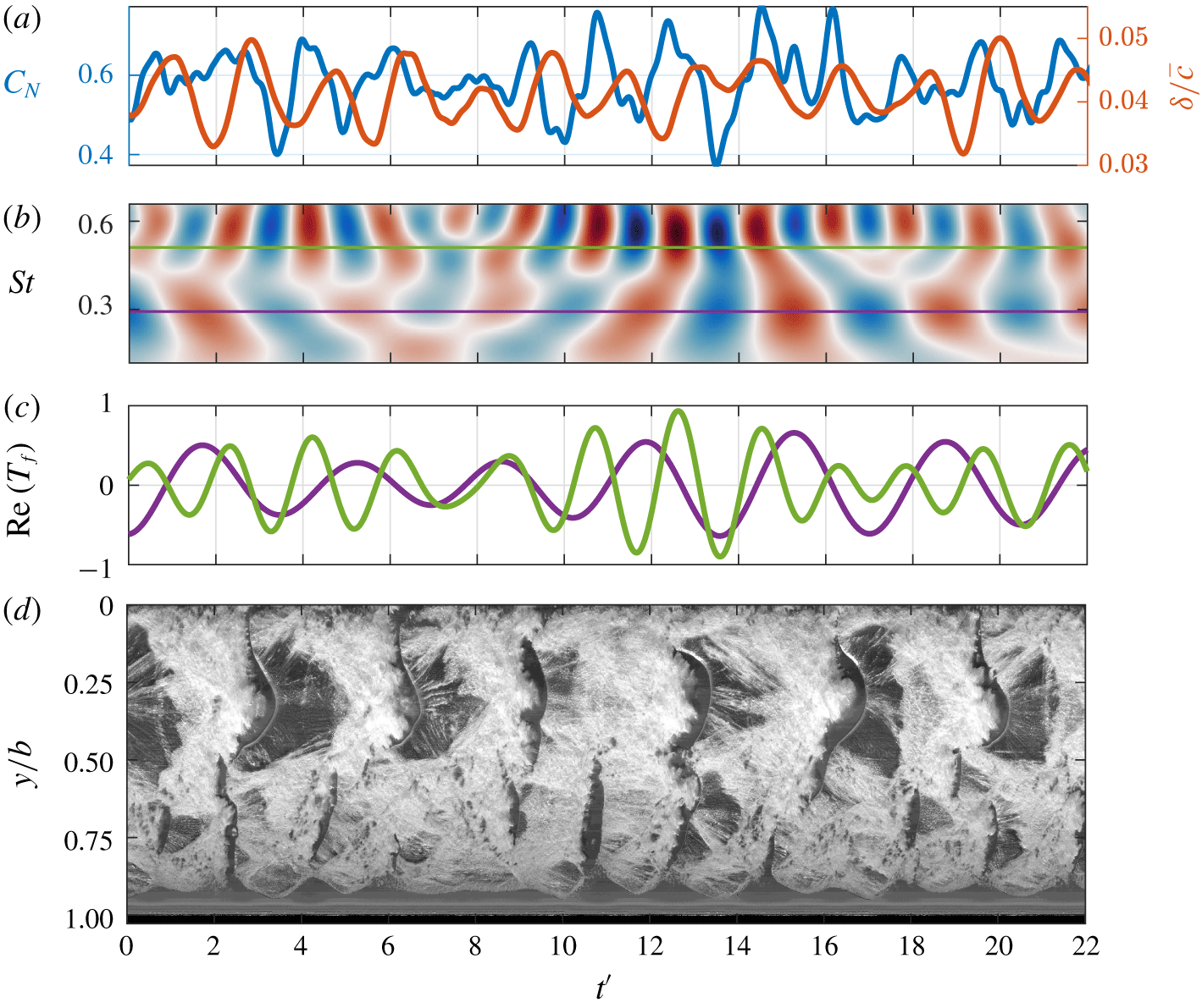
 $\unicode[STIX]{x1D70E}=0.6$. The increased cavity length and width of the shedding cavitation clouds are no longer compatible with the hydrofoil span to form multiple stable shedding sites. This results in a single periodic shedding site in the upper half of the span, as evident in the space–time plot in figure 15(c). In the lower half, the cavity is shed at the same frequency, albeit with less energy (figure 10).
Synchronised time series of the normal force ( $C_{N}$) and tip displacement (
 $\unicode[STIX]{x1D6FF}/\bar{c}$) (a) with the real value of the Morlet wavelet transform for
 $C_{N}$ (b) at
 $\unicode[STIX]{x1D70E}=0.6$. The hydrofoil experiences a relatively consistent
 $St=0.22$ oscillation due to the Type IIa shedding as shown in the spanwise space–time plot taken at
 $x/c_{root}=0.5$ (c). Irregular shedding of small-scale structures in the lower half of the span result in inconsistent and varying intensities at higher frequencies evident in the wavelet transform.

At  $\unicode[STIX]{x1D70E}=0.6$, the attached cavity has reached the trailing edge with
 $L_{c}/c\approx 1.0$ at all spanwise positions (figure 6). Shortly after which the centre of pressure starts shifting back towards the leading edge with further reduction in
 $\unicode[STIX]{x1D70E}$. This is attributed to the suction side increasingly experiencing a uniform
 $p_{v}$ pressure distribution along the chord due to the attached cavity. This increases the relative contribution of the fully wetted side’s pressure distribution, shifting
 $x_{cop}$ back towards the leading edge, as shown in figure 7.
With the cavity reaching the high-pressure region near the trailing edge and closing in a region with a low adverse pressure gradient, the shockwave instability becomes active in the flow at low  $\unicode[STIX]{x1D70E}$. As the cavity grows, the re-entrant jets forms and progresses upstream, slowing down as it approaches the upstream extent of the attached cavity and stalling before it causes the cavity to detach. The re-entrant jet behaviour causes perturbations to form over the attached cavity as it grows with small-scale break-up generating a bubbly flow in the region with a high void fraction, shown in supplementary movie 5. This preconditions the flow for condensation shockwaves to propagate upstream from the collapse of the cavity as it reaches the higher-pressure region downstream of the trailing edge. Preconditioning of the flow allows shockwave propagation to cause the shedding of cloud cavitation where the re-entrant jet instability drives the shedding frequency, therefore showing a dependence on
 $\unicode[STIX]{x1D70E}$ with frequency dropping non-linearly with
 $\unicode[STIX]{x1D70E}$ (figure 8).
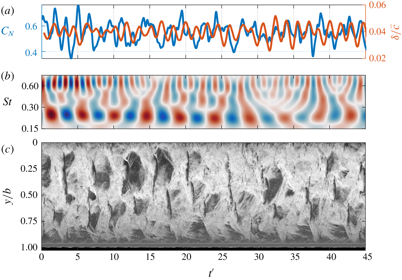
As  $\unicode[STIX]{x1D70E}$ is reduced to 0.5, the shedding frequency decreases in a non-linear trend to
 $St=0.19$ with induced
 $C_{N}$ fluctuations becoming more consistent as evident in the
 $C_{N}$ wavelet transforms for
 $\unicode[STIX]{x1D70E}=0.6$ and
 $0.5$ in figures 15(b) and 16(b), respectively. This is due to the larger cavity influencing more of the span, as evident in the SPOD intensity maps of
 $\unicode[STIX]{x1D70E}=0.5$ and
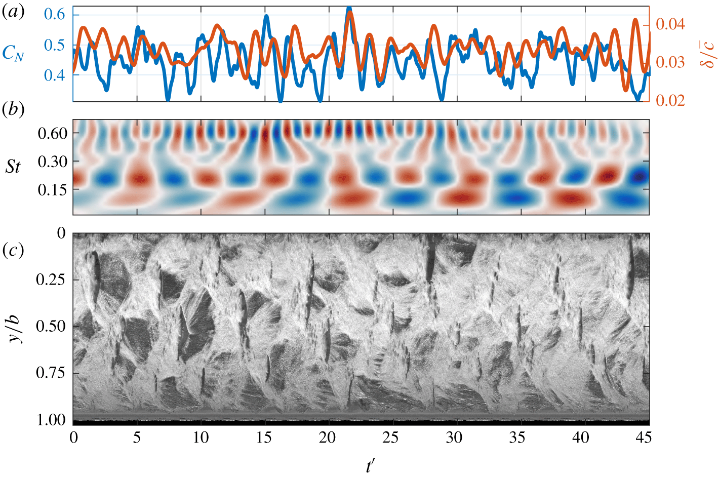
 $0.6$ (figure 10). This increased coherent spanwise activity is due to several shedding events (of similar length scale and hence frequency) starting near the root and then occurring successively out along the span. This is shown in the space–time plot (figure 16c) by groups of 3–4 gaps in the cavitation per cycle, starting at the top and moving down in a regular sequence. This is shown to occur 8 times in the space–time plot from
 $t^{\prime }=0$ to 45, resulting in an approximate frequency of 20 Hz, or
 $St\approx 0.19$, matching the
 $C_{N}$ and
 $\unicode[STIX]{x1D6FF}/\bar{c}$ spectra.
Synchronised time series of the normal force ( $C_{N}$) and tip displacement (
 $\unicode[STIX]{x1D6FF}/\bar{c}$) (a) and the real value of the Morlet wavelet transform for
 $C_{N}$ (b) at
 $\unicode[STIX]{x1D70E}=0.5$. The spanwise space–time plot (c) taken at
 $x/c_{root}=0.5$ reveals multiple shedding events along the span and the complex cavitation behaviour.

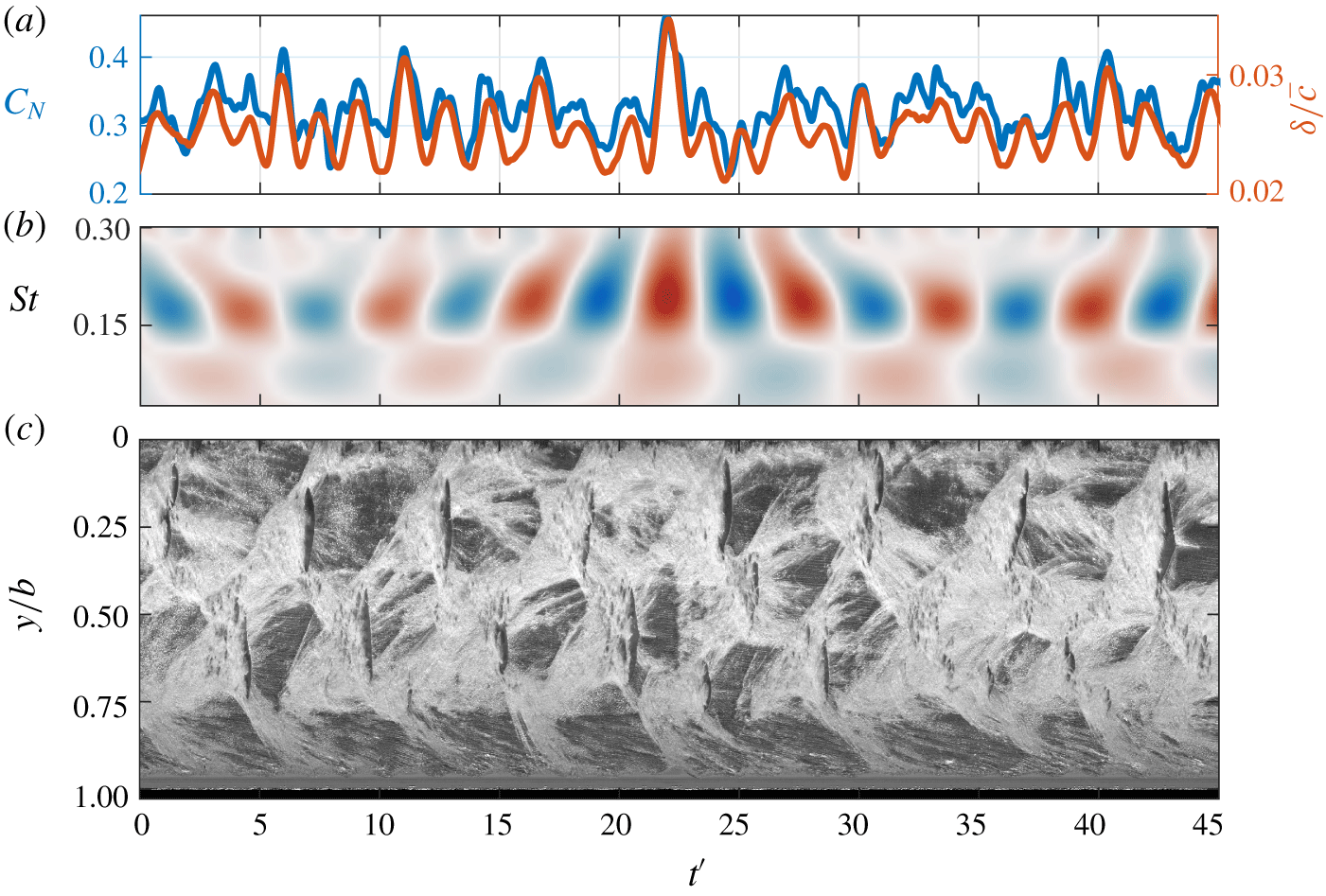
The Type IIa shedding is apparent down to  $\unicode[STIX]{x1D70E}=0.4$ where the attached cavity extends beyond the hydrofoil’s trailing edge before detaching periodically at
 $St=0.17$, evident in the
 $C_{N}$ and
 $\unicode[STIX]{x1D6FF}/\bar{c}$ spectra. Observations from the space–time plot in figure 17(c) and supplementary movie 6 indicate an alternating shedding behaviour where a cloud is shed from the upper portion of the span (
 $0.0<y/b<0.4$), followed by a cloud from the lower portion. This has manifested in the SPOD intensity and phase maps where two primary energetic areas that appear on the planform are out of phase for
 $St=0.16$.
Synchronised time series of the normal force ( $C_{N}$) and tip displacement (
 $\unicode[STIX]{x1D6FF}/\bar{c}$) (a) at
 $\unicode[STIX]{x1D70E}=0.4$, showing strong correlation, with the real value of the Morlet wavelet transform for
 $C_{N}$ (b) highlighting the dominant
 $St=0.17$ oscillation. Spanwise space–time plot (c) taken at
 $x/c_{root}=0.5$ shows the alternating shedding behaviour.

3.4.5 Shockwave-driven shedding
The onset of shockwave propagation occurs as  $\unicode[STIX]{x1D70E}$ is reduced to
 $0.6$ where the cavity length is now about equal to the chord,
 $L_{c}\approx c$, and closes in a relatively weak adverse pressure gradient. The increased size of the attached cavity results in larger cavitation clouds being shed which have a sufficient bubble population and void fraction to permit shockwave formation. This occurs when the cloud is advected downstream of the trailing edge into a high-pressure region where the cluster of bubbles collapse coherently. The bubbles from the larger cavitation clouds at the reduced
 $\unicode[STIX]{x1D70E}$ also increase the local void fraction to the point that the speed of sound in the bubbly mixture reduces significantly compared to that of the constituent water, air and vapour (Shamsborhan et al. Reference Shamsborhan, Coutier-Delgosha, Caignaert and Nour2010). This makes the compressible liquid–vapour mixture susceptible to condensation shocks suddenly changing the local void fraction as the shock propagates through the medium (Crespo Reference Crespo1969; Noordzij & Van Wijngaarden Reference Noordzij and Van Wijngaarden1974; Brennen Reference Brennen2005; Ganesh et al. Reference Ganesh, Mäkiharju and Ceccio2016).
The  $C_{N}$ and
 $\unicode[STIX]{x1D6FF}/\bar{c}$ spectra show that both Type I and Type IIa modes are evident for
 $0.4\leqslant \unicode[STIX]{x1D70E}\leqslant 0.6$ with the co-existence of re-entrant jet and shockwave instabilities. This complex mix of shedding mechanisms has previously also been observed by de Graaf et al. (Reference de Graaf, Brandner and Pearce2017) and Smith et al. (Reference Smith, Venning, Brandner, Pearce, Giosio and Young2018). High-speed photography also reveals the presence of both mechanisms, where the shedding cycle starts with the typical re-entrant jet process with flow moving upstream under the cavity. However, due to the increased void fraction promoting shockwave propagation with the collapse of the previously shed cavity, the downstream extent of the cavity starts breaking up into a bubbly mixture as the shockwave propagates upstream. In the case of
 $0.5\leqslant \unicode[STIX]{x1D70E}\leqslant 0.6$, the re-entrant jet is the primary driver of the shedding frequency with detachment of the cavity coming from shockwave propagation through the preconditioned flow. The SPOD intensity map for
 $\unicode[STIX]{x1D70E}=0.4$ at
 $St=0.11$ indicates that activity in the cavitation due to the shockwave is located at the downstream extent of the cavity, a region of relatively high pressure. However, shockwave propagation is not evident in the space–time plots at a frequency of
 $St=0.11$ with the minimal amplitude in the wavelet transform component shown in figure 17(b), despite appearing in the
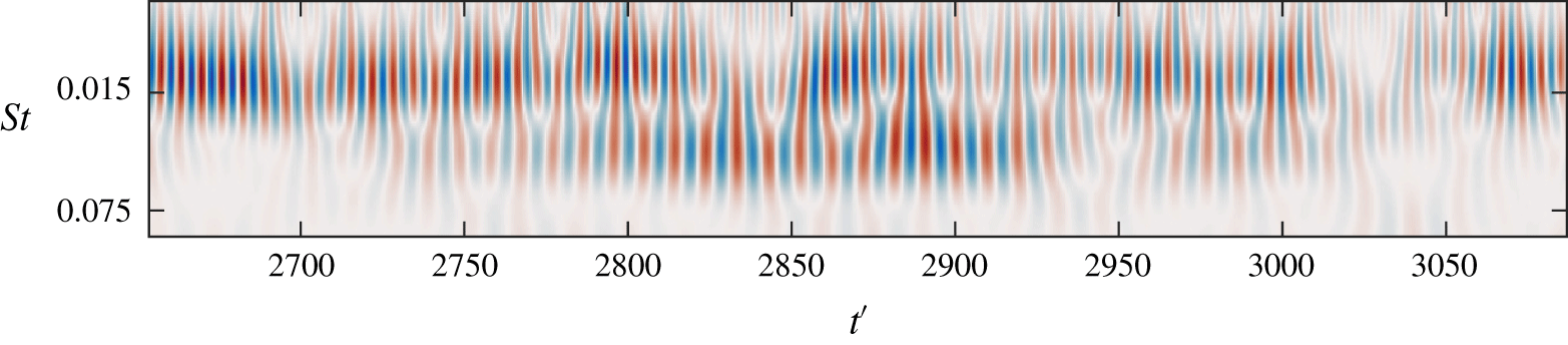
 $C_{N}$ PSD in figure 9. This is due to the intermittent nature of the global Type I shockwave instability being inactive for periods on the scale of seconds as can be seen in the wavelet transform from the medium type run at
 $\unicode[STIX]{x1D70E}=0.4$ (figure 18). As the short type run acquisition is only one second in duration, the data presented in figure 17 have seemingly not included one of the intermittent Type I shockwave events. Alternatively, a space–time diagram produced from the medium run data, due to the reduced frame rate, lacks sufficient resolution to show clearly the Type I shockwave propagation.
Real value of the Morlet wavelet transform for  $C_{N}$ from the medium duration run at
 $\unicode[STIX]{x1D70E}=0.4$. The shockwave-driven low mode (
 $St\approx 0.11$) is not continuously apparent through time, only being evident in the range
 $2800\leqslant t^{\prime }\leqslant 2950$.

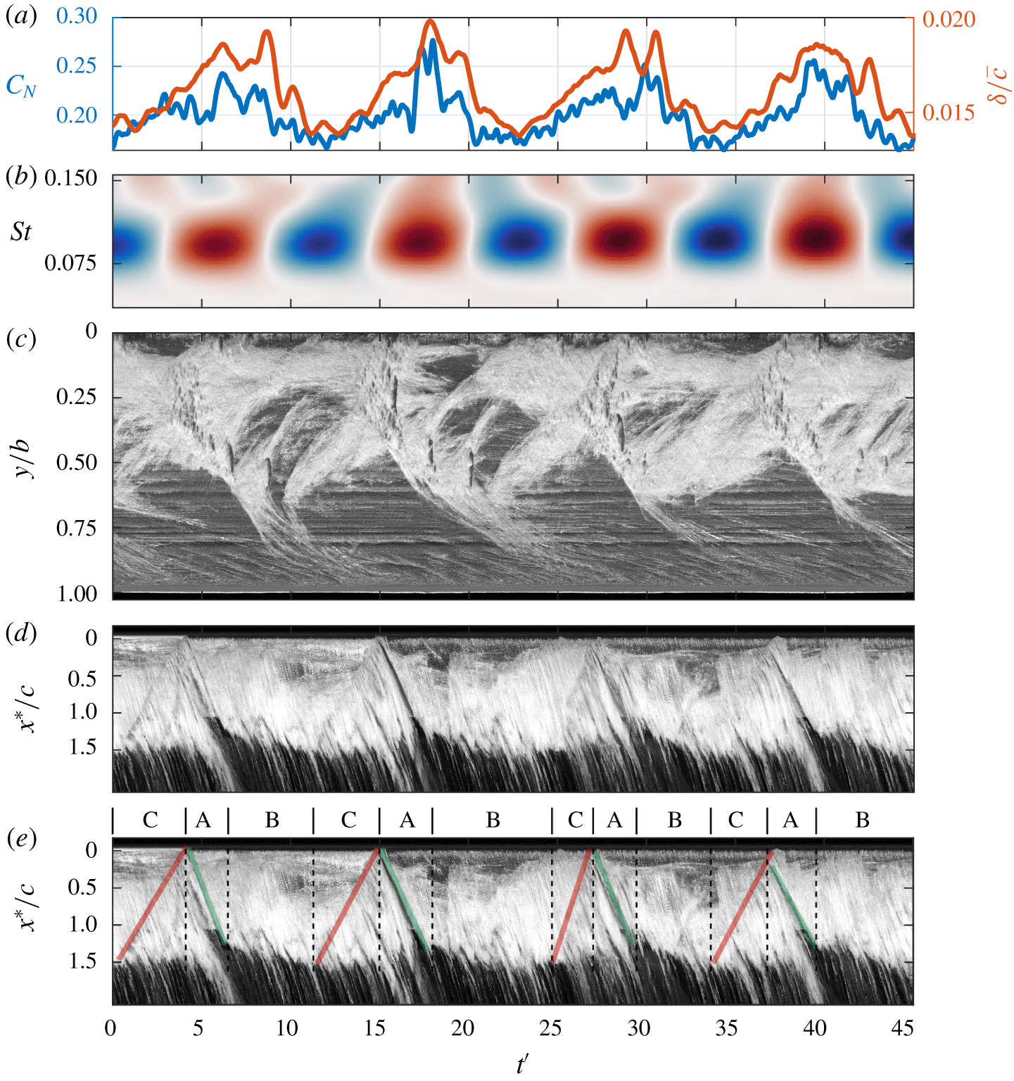
Synchronised time series of the normal force ( $C_{N}$) and tip displacement (
 $\unicode[STIX]{x1D6FF}/\bar{c}$) (a) at
 $\unicode[STIX]{x1D70E}=0.3$, showing strong correlation, with the real value of the Morlet wavelet transform for
 $C_{N}$ (b) highlighting the dominant
 $St=0.09$ oscillation. Spanwise (c) and chordwise (d,e) space–time plots taken at
 $x/c_{root}=0.5$ and
 $y/b=0.25$, respectively, reveal that each cycle consists of a growth phase (A), indicated by green lines, a stable phase (B) and a shockwave phase (C), indicated by red lines in the annotated version of the chordwise space–time (e).

Further reduction in  $\unicode[STIX]{x1D70E}$ to
 $0.3$ sees the cavity grow to the point that the re-entrant jet-driven Type IIa mode becomes no longer evident in the spectrum (figure 9). High-speed photography reveals a re-entrant jet still forms, however, this has insufficient time and momentum to reach the upstream extent of the cavity before the shockwave, thus preventing it from driving the shedding frequency. The shedding cycle is comprised of a complex set of events consisting of three main phases, a growth phase, a stable phase and a shockwave phase. These phases are noted as A, B and C, respectively, in the annotated chordwise space–time plot of figure 19(e) where the chordwise position is presented locally as
 $x^{\ast }/c$, where the streamwise position,
 $x^{\ast }$, is taken from the leading edge at the spanwise location and
 $c$ is the local chord. The space–time plot shows that the growing cavity pauses once it reaches a point just downstream of the trailing edge, remaining stable for a variable amount of time between cycles, ranging from
 $t^{\prime }=4.3$ to 10.7 in duration. This is followed by the attached cavity being broken up by upstream shockwave propagation. The propagation velocity is seen to change between cycles as indicated by the gradient of the red lines in figure 19(e). The spanwise space–time plot (figure 19c) and supplementary movie 7 shows that a cycle also consists of a large-scale cloud that is shed from the upper portion of the span, shortly followed by approximately two small-scale clouds shed in quick succession from about mid-span. This shedding sequence also manifests in the SPOD phase map at
 $St=0.09$ (figure 10) with small-scale clouds just below mid-span showing a significant phase difference in the high intensity region.
The frequency of the Type I mode does not vary significantly with  $\unicode[STIX]{x1D70E}$. This is due to the shockwave initiation location being relatively invariant with
 $\unicode[STIX]{x1D70E}$ and consequently the distance the shockwave must travel to break off the attached cavity. This is in contrast to the re-entrant jet which must travel the length of the attached cavity which does vary with
 $\unicode[STIX]{x1D70E}$. When acting exclusively, shockwave-driven shedding is highly periodic as shown by the
 $C_{N}$ wavelet transform in figure 19(b) exhibiting a consistent
 $St=0.09$ excitation frequency through time, despite complex spanwise cavitation behaviour.
3.4.6 Supercavitation
The reduction of  $\unicode[STIX]{x1D70E}$ from
 $0.3$ to
 $0.2$ sees a significant growth in the cavity length to
 $L_{c}/c>1.5$, now forming a super-cavity (figure 5). Closing far downstream of the trailing edge with no strong adverse pressure gradient present, the super-cavity becomes more stable than partial cavities as no substantial shedding mechanisms can form. In addition, the associated turbulence and vortex shedding occurs far enough downstream to have negligible influence on the hydrofoil and the forces it experiences (Brennen Reference Brennen1995).
The Type I mode disappears as the hydrofoil experiences supercavitation exhibiting no significant peaks in the  $C_{N}$ and
 $\unicode[STIX]{x1D6FF}/\bar{c}$ spectra (figure 9) as no large-scale shedding events are observed in the high-speed photography (supplementary movie 8), despite the vapour cavity remaining in a relatively high-pressure region. As mentioned previously, growth in the attached cavity leads to a higher void faction in the local flow, reducing the speed of sound below the local flow speed and allowing shockwave propagation. However, the speed of sound will actually increase in a liquid–vapour mixture if the void fraction is high enough (Shamsborhan et al. Reference Shamsborhan, Coutier-Delgosha, Caignaert and Nour2010). Reducing
 $\unicode[STIX]{x1D70E}$ to
 $0.2$ appears to have increased the void fraction sufficiently, inhibiting the remaining primary shedding instability from inducing periodic cloud cavitation. With no instability to break up the attached cavity, the cavity grows significantly (figure 6), closing far downstream to form a stable super-cavity.
3.4.7 Spanwise cavity oscillation
Experiments conducted on the same hydrofoils by Pearce et al. (Reference Pearce, Brandner, Garg, Young, Phillips and Clarke2017) observed streamwise cavity oscillations not related to re-entrant jet or shockwave mechanisms, attributing them to spanwise tip excursions. The attached cavities are observed to oscillate, not just in the streamwise direction, but the spanwise direction as well, when the hydrofoil experiences cloud cavitation. Space–time plots taken around the quarter chord show the spanwise cavity oscillations which appear to be highly periodic (figure 20). They also do not appear to be directly related to shedding physics evident in the upper portion of the plots.
Spanwise space–time plots for various  $\unicode[STIX]{x1D70E}$ showing the spanwise cavity oscillation towards the tip of the hydrofoil. These oscillations are periodic and show a strong correlation with the tip displacement.

The spanwise growth and contraction of the cavity was recorded using a column of pixels at a specific chordwise location with tracking of the cavity extent achieved using the same edge detection method utilised for tip deflection measurements. Comparison of the PSD from the resulting time series with that of  $\unicode[STIX]{x1D6FF}/\bar{c}$ (figure 21) reveals highly similar spectra, indicating a strong correlation between tip displacement and spanwise cavity oscillations. Additionally, apart from the lock-in phenomena (at
 $0.65\leqslant \unicode[STIX]{x1D70E}\leqslant 0.75$), this is the only clear manifestation of structural excitations in the cavitation behaviour with the spanwise cavity oscillations being the only aspect exhibiting fluctuations for
 $St\geqslant 0.55$ that is not attributed to shedding instabilities. This is an indication that the influence of FSI on the cavitation behaviour with the stainless steel model is almost inconsequential, therefore reinforcing its validity to serve as a relatively stiff reference.
PSD of the spanwise cavity oscillations compared to that of the  $\unicode[STIX]{x1D6FF}/\bar{c}$ showing similar spectral content at all
 $\unicode[STIX]{x1D70E}$, indicating a strong correlation between the two.

4 Conclusion
The behaviour of various cavitation regimes about a relatively stiff hydrofoil was investigated using high-speed photography and force measurements. Multiple cavitation regimes occurred in the cavitation number range tested, comprising of sheet, cloud and supercavitation, each exhibiting unique traits. The instabilities driving the cavity shedding were identified from high-speed photography as either interfacial instabilities, re-entrant jet formation, shockwave propagation or a complex, coupled mechanism, depending on the cavitation number. Three primary shedding modes were identified with the Type I shockwave-driven shedding oscillating at a frequency nominally independent of  $\unicode[STIX]{x1D70E}$. Re-entrant jet-driven Type IIa and Type IIb oscillations exhibit a non-linear dependence on
 $\unicode[STIX]{x1D70E}$, decreasing in frequency with
 $\unicode[STIX]{x1D70E}$ due to growth in cavity length. At higher cavitation numbers (
 ${>}1.0$) where the cavity length is small, break-up is driven by small-scale interfacial instabilities that leads to small vapour pockets being shed. Reduction in
 $\unicode[STIX]{x1D70E}$ to 1.0 moves the cavity closure into a region of sufficient adverse pressure gradient for a re-entrant jet to form and drive medium-scale shedding from mid-span. For cavitation numbers between 0.9 and 0.7, the streamwise length of the cavity is geometrically compatible with the hydrofoil span to form two stable periodic shedding modes, Types IIa and IIb, driven by a re-entrant jet instability towards the root and tip, respectively. Decreasing the cavitation number below 0.6 sees the emergence of a shockwave instability with the cavity reaching the high-pressure region at the trailing edge and reducing the local speed of sound below the local flow speed by increasing the void fraction. The re-entrant jet and shockwave instability occur concurrently, both causing complex shedding physics and behaviour for
 $0.3\leqslant \unicode[STIX]{x1D70E}\leqslant 0.6$ with the Type I shockwave-driven shedding being the sole shedding mechanism remaining for
 $0.25\leqslant \unicode[STIX]{x1D70E}\leqslant 0.3$. Further reduction in
 $\unicode[STIX]{x1D70E}$ to 0.2 sees the cavity grow to a point that it closes far enough downstream to form a stable super-cavity as no shedding mechanisms can form. Lock-in is seen to occur at
 $0.65\leqslant \unicode[STIX]{x1D70E}\leqslant 0.75$ with the Type IIa shedding frequency matching the first sub-harmonic of the hydrofoil natural frequency in cavitating conditions. Despite lock-in, the structural deformations remained relatively small compared to hydrofoil dimensions and were observed to have minimal effect on the cavitating behaviour only manifesting in spanwise cavity oscillations. Hence, the stainless steel model provides a relatively stiff reference model for comparison with, and to aid in interpretation of, a more flexible hydrofoil of the same geometry. These results will be presented as a Part 2 to the present report in a follow on publication.
Acknowledgements
This project was supported by the Research Training Centre of Naval Design and Manufacturing (RTCNDM), US Office of Naval Research (Dr K.-H. Kim, Program Officer) and ONR Global (Dr W.-M. Lin) through NICOP S&T grant no. N62909-11-1-7013. The RTCNDM is a University-Industry partnership established under the Australian Research Council (ARC) Industry Transformation grant scheme (ARC IC140100003). The authors would like to acknowledge the assistance of Mr S. Kent and Mr R. Wrigley from the Australian Maritime College for their essential help with setting up and carrying out the experiments.
Declaration of interests
The authors report no conflict of interest.
Supplementary movies
Supplementary movies are available at https://doi.org/10.1017/jfm.2020.321.