

There is general agreement that turnout tends to be higher in countries with proportional representation (PR) than in those with single-member plurality (SMP) electoral systems, all other things being equal.Footnote 1 There is disagreement on the size of the effect, the plausibility of explanations for it, and how robust it may be.Footnote 2 Differences between electoral systems can be identified and analysed on a cross-sectional basis using aggregate country-level data or micro-level datasets such as those from the Comparative Study of Electoral Systems (CSES). But it would be helpful to confirm that such differences can also be found when systems change over time. In principle, the same theoretical logic should apply to cross-sectional and temporal comparisons. There are a limited number of cases of major electoral system change, limiting the opportunities for time series analysis. We still know little about many of the medium to long-term effects.
The effects of electoral system change on turnout over time can be estimated in New Zealand, making it a ‘critical case’. After nearly a century of SMP elections, New Zealand changed in 1996 to a Mixed Member Proportional (MMP) system, and has since held five elections, the most recent in 2008. Under MMP, there are two votes. There is a party vote for national lists that is used to allocate the total number of seats for each party according to the Sainte-Laguë formula. From these lists, for example, in 2005 fifty-two seats were allocated on a compensatory or ‘top up’ proportional basis after the tallies of the other vote, the electorate vote, had determined the candidates elected in the other segment of the system made up of sixty-nine single-member districts. With a 5 per cent party vote threshold, also crossed by winning a constituency seat, New Zealand’s MMP therefore qualifies as a PR system, although its mixed nature needs to be kept in mind.Footnote 3 As a critical case of electoral system change, New Zealand’s institutional experiment is worth analysis in its own right. Whether or not this New Zealand experience can be a source of generalization about electoral system change and electoral system effects more generally remains an open question.
This article now proceeds to review the theoretical background to the question of turnout differences between SMP and PR systems. In the second section, the implications of these theories are considered more deeply in terms of change over time in the New Zealand case, generating a list of hypotheses. In the third section, age cohorts associated with generational effects that recent turnout research has identified empirically are defined and examined. The fourth section defines and reports a multivariate analysis of data pooled over ten New Zealand elections, and the fifth concludes and summarizes the findings.
The Theoretical Background
Analysis of turnout is normally conducted at the macro or the micro level. This analysis operates at both these levels, although the macro cases are elections within one country, rather than countries and elections. While different explanatory variables tend to be brought to bear at the macro and micro levels, in principle the theory at the foundation of the analysis should come from the same source. The point of departure here is rational choice institutionalism, in which the basic utility-maximizing rational choice model identifying costs (C), benefits (B), and the probability a vote of having an effect (P) is supplemented by inferences about the incentives created by different institutional arrangements (I). While it is acknowledged that this approach has some difficulty in explaining a high level of individual-level variance in the choice to vote or not to vote, it is much more powerful when addressing change on the margins, the main focus here.Footnote 4 In addition, the theory can also draw on political learning or socialization effects, particularly as these apply in the experiences of political generations or age cohorts.
The last two decades of research on electoral turnout indicate that while most of the effects of PR appear positive, countervailing elements complicate the relationship. Positive effects include higher perceptions of efficacy under PR, particularly among minorities and those who prefer small parties, who may be able, or who at least may feel it more likely that they can elect people to represent them, another influence on P and also on B. A wider range of parties to choose from may bring out people who are otherwise less likely to vote.Footnote 5 Perhaps most important, votes under PR are far more likely to ‘count’, even when cast for losing or non-government parties, due to greater national competition and higher district magnitude, a P effect again. Put the other way around, under PR far fewer people have reasons to believe that their vote will not count. The higher the district magnitude, the less likely it is that anyone can calculate whether or not their vote will make a difference to a seat allocation.
But to the extent that PR systems generate multi-party systems and coalition governments, there can be a negative effect on turnout. Party system fragmentation can make the formation of governments less predictable and transparent, influencing P in the other direction, in terms of a choice of government.Footnote 6 The formation and breakdown of New Zealand’s first coalition government under MMP led to such perceptions.Footnote 7 At first sight, PR systems might be assumed to enhance mobilization, thus minimizing C. But local party contacts to mobilize voters happen less, because increasing district magnitude lowers the incentives and increases the costs for individual candidates to get out the vote, an I factor.Footnote 8 A mixed-member system with an SMP component under PR could conceivably retain some of those advantages. Meanwhile, party preferences appear to be stronger under PR,Footnote 9 presumably offsetting the deficiencies of mobilization. A balanced or mutually offsetting mixture of these various effects could mean that the consequence of change of electoral system might not be a turnout effect, or at least not a major one.
As foreshadowed above, models explaining turnout must now recognize that elections within a country case are themselves cases at a lower level, with individuals sampled in election surveys at a lower level again. For present purposes, elections within countries should be seen as ‘conditional cases’ in a multi-level model on individual vote or no vote. They contribute independent variables at the macro level that are hypothesized to affect the dependent variable nested at the micro level. One should also note that the elections examined here are not a sample but a universe, at least in the sense of making generalizations about post-MMP New Zealand elections. Therefore, they should not be seen as constituting a dataset subject to tests of statistical significance, but are rather more equivalent to data generated in a small-N case study research design.Footnote 10
Elections are important cases because they form the framework through which to apply macro-level controls, and particularly to address what Mark Franklin identifies as ‘the primacy of electoral competition’ (once more, P).Footnote 11 This article takes on board much of the Franklin model, seeks to deepen its ‘take’ on the New Zealand case, but adds a note of scepticism about one of its assumptions. Franklin’s model is particularly relevant to the effects of electoral system change because, drawing on theories of political learning, it implies a modification of the rational choice model by suggesting that there could be a lag effect: behaviours learnt under one set of conditions of B, C and P may not quickly adjust to new ones. Franklin emphasizes this effect upon younger voters, but other may be affected too.Footnote 12 The model is also highly relevant because a change of electoral system changes the conditions of party competition, and thus P. Where the most competitive contests take place in a minority of closely contested single-member districts, turnout is likely to be lower than it would be where the whole country is a single electoral district that elects members from party lists under PR.
Applying The Theory To The New Zealand Case
The New Zealand case challenges electoral systems theory and previous empirical studies, as turnout has continued a long-term decline under the new MMP system. Figure 1 tracks valid vote/age-eligible turnout in New Zealand, the most appropriate means of estimating electoral participation in New Zealand.Footnote 13 Around the middle of the twentieth century, New Zealand’s turnout rates were remarkably high for a country without compulsory voting. After a steady fall up to 1966 accompanied by the beginnings of a process of party dealignment, electoral participation recovered up to 1984, moderately high by international standards, but no longer stratospheric.
Electoral Turnout in New Zealand, 1946–2005 Note: Valid votes on a base of age-eligible turnout.

Turnout dropped steeply in 1987 and 1990, and recovered only slightly in 1993 for the last SMP election, at which a referendum on the shift to MMP was held, perhaps encouraging a small turnout increase. Turnout increased again at the first MMP election in 1996.Footnote 14 But two declines followed with turnout at 71.7 per cent in 2002 and a recovery in 2005 back up to 76.1 per cent: still lower than at the first MMP election in 1996.Footnote 15 In 2008, valid vote/age-eligible turnout fell again to 74.7 per cent. New Zealand can no longer be said to have an exceptionally high turnout, as it did in the 1940s and 1950s. At best, for a country of its size, the current level can be described as slightly higher than ‘ordinary’. Average turnout for the first four elections under MMP was 75.3 per cent. For the last four elections under the SMP system, it was 79.6 per cent. On the very surface, the claim that turnout should be higher under a PR system appears to be refuted.
Models that estimate a PR turnout advantage on a cross-sectional basis do so with appropriate control variables. Analysis over time should do the same. Taking into account other effects that might be driving decline, turnout under MMP could still be higher than it would have been under SMP. Changes in social structure could increase or decrease turnout, if social groups consistently facing different levels of B and C increase or decrease in size over time. Of more theoretical salience, there are two key variables that separately or together could account for turnout decline: electoral competitiveness and age cohort effects driven by the lag effects noted earlier. From the Franklin model, one can first hypothesize that changes in the closeness of party competition could be part of an explanation for turnout decline under PR. Defining ‘competition’ for present purposes admittedly poses some problems, as there is some debate about appropriate indicators of competitiveness across different electoral systems. One of Franklin’s definitions is the average difference between the two major parties across all electoral districts under SMP systems, with PR systems scoring 0, on an assumption of full competition under that system. Thus, he drops an electoral system variable from his models, subsuming those effects into competition. But while PR may, by definition, be more competitive, between elections there is still significant variation in competition within a PR system, as Franklin also recognizes. The analysis that follows tests whether competition has turnout effects when defined as the margin between the two main parties in national vote share. If it does, this estimator can at least be defended on pragmatic grounds.Footnote 16
Meanwhile, as district-level competition continues in a mixed system, some effects may persist at that level. As all the datasets analysed here include district-level codes for elections t and t−1, these effects can be modelled at the individual level across the experience of electoral system change. One expects that perceptions of electoral competition at time t, however defined, will have direct effects on the probability of voting at time t. And because the extent of competition at time t is conditioned by competition at the election at t−1, that should also have direct effects at time t. Indeed, its effects should be greater because it is known rather than anticipated, and has shaped the political arena immediately prior to t. As pre-election polls are more likely to update perceptions of national competition, competition effects at both t and t−1 are worth estimating separately.
A life-cycle effect has been widely identified in most research on turnout, with young people less likely to vote but more likely to do so as they grow older and perhaps becoming more conscious of B. But there is more recent evidence from various countries that persistent trend effects in patterns of turnout are driven by differences in behaviour between age cohorts.Footnote 17 Various explanations are adduced, notably declining ‘civic duty’ in successive generations, or declining party identifications, but these are either tautology or simply set the need for explanation one step back. With a combination of political learning and the P element of rational choice theory, in another key component of his argument Franklin argues that generational differences may be based on the extent of electoral competition prevailing when people first have the opportunity to vote, thus leading to the interaction of historical competition with age cohort effects. The level of turnout so influenced, Franklin argues, plants a ‘footprint’ on subsequent behaviour. The lowering of the voting age, in particular, is said to have had a detrimental effect on turnout because those affected were not old enough to be sufficiently integrated into the social networks that lower the costs and bring attention to the benefits of electoral participation.Footnote 18
If competition has declined over time, and there is sufficient stability in behaviour within age cohorts, older age cohorts will have higher turnout habits, and younger age cohorts will have lower turnout habits that persist as their members grow older. Therefore, turnout will decline. Contextual and institutional changes may affect all voters to some extent, but the footprint of early experience will make trends of change ‘sticky’. Smoothing out the data, there is some evidence of declining national electoral competition in New Zealand over the last half of the twentieth century, but there is great variation from one election to the next.Footnote 19 If the youth footprint theory holds, election-contextual and institutional change will most influence people entering the electorate. They are most likely to take an imprint of either higher or lower turnout. If it significantly enhances perceptions of electoral competition, the change to proportional representation could increase turnout among new voters most open to new habits but have little or no effects on older generations among whom turnout habits are already imprinted.
Derived from a combination of the rational choice institutionalism and political learning theories explained above, the hypotheses can now be summarized as follows:
Hypothesis 1. Age-cohort effects may affect turnout more than life-cycle effects.
(a) If there is a trend of declining electoral competitiveness, it will set a pattern of long-term turnout decline.
(b) Those belonging to age cohorts entering the electorate after the lowering of the voting age will have a similarly lower probability of voting.
(c) Otherwise, age-cohort differences are driven by turnout at the time those age groups entered the electorate.
Hypothesis 2. As electoral system change affects the nature of electoral competitiveness, there will be a positive effect for PR on turnout, the strongest among people in the early stages of their voting life under PR.
Hypothesis 3. Other things being equal, turnout under PR should be higher than under the SMP system.
Hypothesis 4. Estimated directly, electoral competitiveness at times t and t-1 will directly affect levels of turnout.
(a) Under PR, the extent of national competition will have the strongest effect, most likely at time t given the influence of polls.
(b) Under the old SMP system, competitiveness at the level of the electoral district will have the strongest effect, most likely at time t−1 because district-level information is mostly derived from the last election.
These hypotheses are tested with pooled data from the successive New Zealand Election Studies (NZES), and other earlier data (see Appendix). NZES from the 2008 election is not yet available. Vote or not vote is based on validated samples from 1990 onward, although this does present some complications for the 2002 and 2005 elections that can be overcome (see Appendix).Footnote 20 Unfortunately, many of the earlier datasets also omit some significant social, demographic and attitudinal variables, including party mobilization, for which there is considerable evidence for turnout effects.Footnote 21
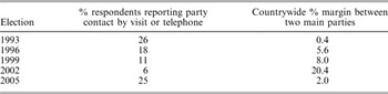
However, Table 1 indicates a close relationship between data on party contact by telephone and visit across the elections from 1993 to 2005. Indeed, party contact correlates with the margin between the two major parties at r = 0.92. We can therefore assume that a national level estimate of two-party competition captures most of the effects of competition.
Competitiveness and Mobilization in New Zealand Elections, 1993–2005

Source: New Zealand Election Studies 1993–2005.
Defining The Age Cohorts
To estimate ‘pure’ generational effects, age cohorts must be defined to reflect the hypothesized effects of different generational experiences affecting the perceptions of B, C and P when voters entered the electorate, perhaps persisting into later life, and thus resisting a more recent competitive context. The effects of competition at the time of entering the electorate can also be modelled separately, as can the level of turnout at that time.
People born before 1933 experienced the Depression, and those born after 1934 and before 1945 grew up during the Second World War and slightly after: these periods define the ‘depression’ and ‘war’ generations. The first year in which the ‘baby boom’ generation was born is understood as 1945. That group is split into those who began voting before the lowering of the voting age, and those who began after. Those born in 1965 entered voting in the 1980s, a period of economic reform and cynicism about government, and are often given the label ‘generation X’. ‘Generation Y’ are those born in 1975 and after, who began voting just before or after the change to MMP.
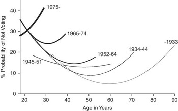
Figure 2 plots turnout by members of these generations by their ages at the election at which they appear in the samples across successive New Zealand election studies. Polynomial curves are drawn across the cross-tabulated data for each generation, age by turnout and merged together into the figure.Footnote 22 The series of elections covered begins in 1963 and was continuous from 1987 but there are significant gaps.Footnote 23 The series includes six elections under the SMP system (1963, 1975, 1981, 1987, 1990 and 1993) and four under MMP (1996 onwards).
Not voting by age in each generation in New Zealand, 1963–2005 Note: Second-order polynomials drawn through not voting by age in each generation. Source: Successive NZES and other election studies (see Appendix).

The figure shows substantial differences between the generations, although not those expected. Because of gaps in the data, and variations in electoral context within each snapshot of generational experience, the patterns need to be interpreted carefully. The depression generation demonstrates the least failure to vote, but only after the age of 45 or so. In 1963, the data for this group begin in the 30s age group upwards, so we do not know the extent to which its members voted when younger, in the 1950s and before. But the slope of the curve suggests that like almost all the generations, about 30 per cent may not have voted at their first election, although this seems high given the health of turnout in the period. The exceptional generation appears to be that of 1945–51, the first wave of the baby boom. Its members would have begun voting in the late 1960s, at a time of high youth engagement in politics, at least reputedly so. However, the earliest data from this group come from 1975 onwards, so again there are no data for the elections when they began to vote. There seems little evidence of a lowered voting age effect that should affect the next cohort, ‘baby boom two’, 1952–64.
Figure 2 presents intriguing data, but the information it provides from early elections is thin. Later, with more elections contributing, it glosses over, or may be distorted by, differences in competition between elections. For example, generation Y’s very different trajectory stands out, probably reflecting declining national competition in the second and third MMP elections. Nonetheless, these patterns cast doubt on the ‘youth footprint’ thesis. Where it can be directly estimated, it seems that turnout among the young has not declined between the successive generations, and that the generational differences have emerged later.
Multivariate Analysis
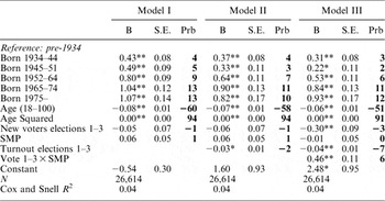
To penetrate more deeply into the combined partial and possibly interactive effects of generations, competition and electoral system change, Tables 2A and B display the findings from six logistic regression models progressively adding sets of the relevant variables and thus ‘decomposing’ the generational and electoral system effects. As before, generations are defined from the year of birth. Life-cycle effects are estimated from age at the time of behaviour, expressed in quadratic terms by the addition of the square of age to the model to capture the non-linear shape of the relationship displayed in Figure 2.Footnote 24 More detailed variable definitions and a discussion of alternative approaches are provided in the Appendix. The first model is based on the variables used to draw Figure 2, plus the identification of new voters and electoral system change. It sums up the effects more clearly than was possible by visual inspection. Against non-voting/voting, it regresses generations and life-cycle effects, respondents facing one of their first three elections, and a dummy variable for SMP or MMP elections.Footnote 25 One should note that this variable is a proxy for the SMP/PR difference, not a direct estimate of its effects.

Probabilities of Not Voting: Cohort Effects, System Change and Competitiveness, 1963–2005

This model partly confirms Hypothesis 1. People in successive generations are progressively less likely to vote when compared to the reference group, the pre-1934 depression generation. The percentage probability figures estimate this effect at the mean age in the samples, in the late 40s, and where the preliminary analysis in Figure 2 identifies the beginning of significant variation. The difference between the baby boom two cohort first affected by the lowering of the voting age and the reference category of those born before 1934 is smaller than that for Generations X and Y. But there remains a significant life-cycle effect. At this stage, there is no new voter effect independent of the life-cycle effects. After taking into account ‘sticky’ generational effects and the variation in the age structure between elections, not voting was 1 per cent more likely under the SMP system. But this estimate is too small for statistical significance, effectively refuting Hypothesis 3.
No significant effects were found when attempting to estimate the competitiveness prevailing when respondents first voted at one of their first three elections.Footnote 26 The second model adds an alternative estimate of the ‘footprint’, an average of turnout at the first three elections the respondents could vote. This did prove significant, but only in the absence of the estimate of competitiveness at the respondents’ first to third elections. The difference between the turnouts at the elections all those surveyed experienced when young is about 15 percentage points. In the first model, this difference has a 2 per cent effect on turnout. With this control, the probabilities that members of the various age cohorts are less likely to vote than the pre-1934 reference group did reduce somewhat. Cohort effects remain strongest on those born after 1975 and starting to vote in the 1990s. This ‘footprint’ variable cannot measure respondents’ behaviour when first voting, only its context, so the effects noted are probably an underestimate. However, it has no association with the extent of competition when those respondents first began voting. If there was a footprint, it did not come from competition, but instead through other unknown contextual factors that enhanced or reduced turnout at that time.
Model III tests Hypothesis 2, regarding the interaction between the change of electoral system and new voters. It suggests that new voters are more likely to vote under MMP, and were less likely to vote under SMP. However, the minimum–maximum probability estimates are difficult to interpret because of the interaction effect, which can sometimes be misleading in non-linear models such as these. When the predicted probabilities of not voting are derived from the model, new voters were indeed less likely not to vote under MMP (16 per cent) and more likely not to vote under SMP (just over 23 per cent), and the two sets of 95 per cent confidence intervals around those probabilities do not overlap. However, there was no difference in the propensity not to vote across the two systems when all voters were taken into account. People voting after their first three elections are slightly less likely to vote under MMP than under SMP, although this effect is too small to register statistically in its own right.
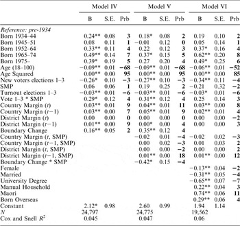
Model IV tests the general principle of Hypothesis 4 and adds competitiveness, measured negatively as the margins across the whole country, and electoral district by district,Footnote 27 between the two largest parties in elections t and t−1. Effects are found for country-level margins at t and t−1, but district margins only have an effect at t−1, the previous election. This supports the inference that a relative absence of polls at the district level means that expectations are driven by the last election, without updating.
This makes sense, and is a far more plausible explanation of the district-level effects of competitiveness in terms of voter knowledge and party mobilization than the margin at the election currently contested. No one can be sure about that until the votes are counted. As for country-level effects, in an era of polls, respondents would have better national-level information about the current election than local-level information about the current situation in their own district, so an effect for current national competitiveness also makes more sense. In this model, turnout at respondents’ first elections has increased effects. The new voter turnout predicted probability differences across the electoral systems slightly increase to nearly 6 points, but the confidence intervals begin to overlap. Model IV also controls for electoral boundary redistributions that take place every five years in New Zealand. All but one election under MMP has been held with new boundaries, a higher proportion than previously under the SMP system. A boundary change tends to increase the percentage not voting by about 2 per cent.
Model V causes the interaction of electoral system differences with the four competitiveness indicators and the timing of boundary changes. The main effects represent the situation under MMP, and suggest that country-level competition is the main driver of turnout under PR, as one would expect with a compensatory party vote. There are signs of a small driver for district-level competition that may be consistent with a limited survival of district-level competition effects in a mixed system. The interactions represent the situation under SMP. They hint that under the SMP system the lagged district margin is the only competitive driver of turnout. It has a quite substantial effect of 18 per cent between the safest and the most marginal electoral district. Generational effects reduce, with the first wave of baby boomers and Generation Y losing statistical significance. New voter effects for electoral system differences remain, but the confidence intervals overlap even more.
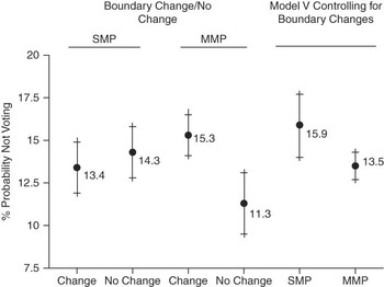
Most notably, the effects of electoral boundary changes appear to differ by electoral system. Under SMP, boundary changes appear to enhance turnout, whereas under MMP they appear to enhance not voting. This may make sense, as there is more incentive for parties to mobilize voters under the SMP system, particularly when boundaries have changed and party organizations are required to adapt. Under MMP, local party organizations have less incentive to be active. But there is an alternative explanation. Party organizations and party memberships have declined over time in New Zealand as elsewhere, and are much weaker under MMP than they were under the SMP system. Thus, their capacity to adapt to boundary changes is weakened, regardless of electoral system differences.
With confidence intervals, Figure 3 plots the predicted probabilities with and without boundary changes under both systems, and estimates the effects of the electoral system on voting or not voting on the basis of Model V. The different effects of boundary changes under the two systems are confirmed. Under SMP, the differences tend to be too small for confidence, but under MMP the intervals do not overlap. Figure 3 also shows that, all other things being equal, turnout should be about 2.5 per cent higher under MMP than it would be under the SMP system. However, the confidence intervals overlap slightly. Moreover, the interpretation of this finding is questionable. It relies on only one MMP election for which there was no prior boundary change that coincided with a turnout recovery and high national competition. If MMP weakens party organizations’ ability to mobilize, the effects of boundary changes are intrinsic to the system and an inappropriate control. Yet, three out of the four MMP elections from the data used here were affected by boundary changes, compared to only three out of the six SMP elections. It does seem plausible that boundary changes will most adversely affect weak party organizations.
Effects of Boundary Changes on the Propensity Not to Vote Under SMP and MMP, and the Predicted Probability of Not Voting After Controls for Generations, Life Cycle, Competitiveness and Boundary Changes Note: Lines represent 95 per cent confidence intervals around the predicted probabilities of not voting. Data derived from Table 2B, Model V, all other independent variables being held at their means.

Adding social structure controls that provide more information about factors that may shape C and B, Model VI provides the most stringent test of the various hypotheses, although it drops all cases from 1963, 1981 and 1987, leaving only three FPP elections against the four MMP elections, opening up some room for doubts.Footnote 28 Dropping these cases makes little difference to an alternative version of Model V, but a choice between the two models is ultimately a judgement call.Footnote 29 The difference in district competition effects is stronger without the social structure controls, because on average the dropped SMP elections tend to have a stronger relationship between turnout and competitiveness than those remaining in the model (see Appendix). Most significantly, Generation Y cohort effects open up again after the addition of social structure controls rather than being further reduced, which might have been the case if social structure formed part of an explanation of the generational differences.Footnote 30 Instead, social structure controls open them out again and remain most significant for Generation X. The effects of competitiveness persist in slightly reduced form after the addition of controls for social structure, all of which have significant turnout effects. New voter effects narrow to 3.5 per cent, and the confidence intervals overlap even more. People qualifying to vote for their first few times by reason of age may vote more under MMP than they did under SMP, but at the end of the process of adding further control variables we cannot be at all sure of this.
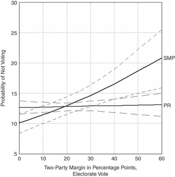
Figure 4 is drawn from the probabilities of not voting under the two different systems at an average level of national competition, extricated from Model VI, with the values of the other variables set at their means. It shows the differences in turnout, shaped by the change of electoral system, between safe and marginal electoral districts. The two sets of 95 per cent confidence intervals separate out at a margin of about 40 percentage points. Over the last four SMP elections, somewhat more than a tenth of the voters were in electorates with margins at that point or higher.Footnote 31 The confidence intervals are particularly wide for SMP because of the smaller number of cases, and due to the exclusion of three SMP elections.
Probability of Not Voting Under SMP and MMP by Electorate Vote Margins Note: Probabilities from model VI calculated at a country percentage margin of 7 points at both t and t−1, all other variables at means. Electorate vote margins calculated as plotted for both t and t−1. Broken lines represent 95 per cent confidence intervals above and below the two main lines. See the Appendix for further details.

But despite the overlapping confidence intervals over most of Figure 4, one can be reasonably confident that the effect is robust. Official data on turnout by electorate under SMP and MMP confirm that competitiveness does matter, and more so when estimated at t−1.Footnote 32 The incentive to vote under the SMP system progressively decreased as electorates became safer for incumbent parties. Under MMP, once other factors such as the greater effects of national competition are taken into account, this effect has almost entirely disappeared. Note also that the confidence intervals separate out again when competition is at its maximum (that is, with non-competitiveness at close to 0). All else being equal, the lack of overlap of confidence intervals at both ends of the lines indicates that turnout may have been higher in electoral districts under the SMP system where the margin was less than 17–18 percentage points, as compared to similarly competitive districts under MMP. This is another likely explanation for the apparent absence of a positive turnout effect under MMP, as up to 35 per cent of electors may be eligible to vote in those districts. However, if there is a turnout difference in the marginal districts that favours the SMP system, it is much smaller than the gap that opens up in safe seats.Footnote 33
The social structure variables indicate aspects of social change over the period, indicating their value as controls. The proportions of the population married and in manual households have declined. People from the indigenous Maori minority population, those with university education and those born overseas have increased. The findings above confirm that the generational differences estimated across the various models have most substantial effects for the two most recent generations: Generations X and Y, those born after 1965, the generations after the one most exposed to the lowering of the voting age.
There is some difference for the second wave of the baby boom, which may be the result of lowering of the voting age to which Franklin ascribes negative effects on turnout.Footnote 34 Yet one should not rule out the potential impact of the cultural changes of the 1960s and 1970s. At the time that many of this group entered or had just entered the electorate in the late 1970s and early 1980s, competitiveness and turnout were high, and political mobilization was increasing both in terms of party membership and activism in social movements.Footnote 35 However, the mobilization effects of the 1960s and 1970s appear to have had their strongest effects on the first wave of baby-boomers who qualified to vote at 21.
As for the two post-1965 generations more prone not to vote, a hypothetical X, a person born in 1965, would have had the opportunity to cast their first vote in 1984, an election characterized by high turnout, moderate competitiveness and a change of government. That government went on to embrace a radical programme of market liberalization that was not signalled or anticipated. A perceived lack of government accountability to the electorate became an issue, turnout began to fall, and dissatisfaction with government peaked in the early 1990s just before the electoral system change. One can hypothesize that the generations beginning to vote since 1984 would begin their political lives with less confidence in the responsiveness of government, and would therefore be less likely to have maintained a habit of voting as they grew older. Limited survey data from the period before the electoral system change makes the testing of this more elaborated version of the ‘footprint’ hypothesis impossible within the models specified here, but a more specific analysis of the under-40 age groups in the post-1987 datasets might pay dividends.Footnote 36
Can a ‘youth footprint’ theory of the habit of voting still hold, even if driven by factors other than electoral competition? If so, one might still expect members of older generations to develop lower expectations about voting, although without such a strong effect on their likelihood of doing so. One can identify each generation with the ages that its members would have experienced the 1980s in a more detailed examination of Figure 2 above. Changes in the expectations of government accountability in the 1980s and the steep turnout declines in 1987 and 1990 appear to have been reflected across all the generations. There is some evidence for a youth footprint and of some ‘stickiness’, but it is not one impressed by the weight of electoral competition when people entered the electorate. There is evidence of a footprint affected by the level of political mobilization at the respondent’s first election. But other evidence suggests that such effects can be eroded. The data currently available to test further conjectures are sparse, and may not be up to the challenge. This interpretation is also vulnerable to question as a single-country specific explanation of a trend found in other countries without the same political experience, or at least without one that was so intense.Footnote 37
Conclusions
In absolute terms, turnout at New Zealand elections fell in 1999 and 2002 for three main reasons. First, in the longer term, there were effects of recent generations with a habit of lower turnout moving into the electorate, while members of older generations with a habit of higher turnout were leaving it. Secondly, subject to short-term fluctuation, there was less competition between the two major parties and this spilled over into declining party mobilization and campaign expenditures, at least until the 2005 recovery on both factors. Thirdly, both elections were held under new district boundaries, and new boundaries impact more heavily under MMP than under the SMP system. While it is impossible to control for the direct effects of campaign mobilization in the pooled models used in this article, most of this is captured by estimates of competitiveness. If lower levels of grass roots mobilization are a feature of list PR, this control is arguably redundant. In 2005, the election was more competitive and was held under the same boundaries as in 2002. Turnout recovered, although not to the level of the last election under the SMP system in 1993. Long-term generational effects have made that level harder to reach even under conditions of relatively high competition. In addition, one can speculate that lower expectations of government accountability laid down in the 1980s and early 1990s may continue to suppress the potential for increasing turnout in New Zealand across all generations, but perhaps somewhat more among those people who began voting at that time, and afterward.
Other things being equal, and despite absolute decline, overall turnout under MMP is no lower than it would have been had the SMP system survived. In the hypothetical absence of system change, it is even possible that turnout in New Zealand under SMP could have fallen slightly lower than under MMP. That said, the evidence for ‘no difference’ is probably strongest. There is robust support for the hypothesis that low competition for the electorate vote in many districts quite strongly discourages turnout under the SMP system, but is also evidence that close district-level competition no longer drives turnout as much as it did under the SMP system. These are well-known features of SMP systems already well understood, but estimated here for the first time in a model allowing direct comparison with the new pattern under MMP. National competition for the PR or party vote has partly offset this disincentive to vote in uncompetitive electorates. New Zealand’s experience with electoral system change provides some further useful insight into the different incentive structures of turnout under SMP and PR conditions. Identification of the different effects of boundary changes under the two systems is almost certainly an original finding that merits investigation cross-nationally. Some combinations of incentives and experiences may enhance turnout more under PR than under SMP. Others may not, and New Zealand, on the best estimates possible, illustrates how the different influences can offset each other.
One more puzzle remains. Current generational patterns may be partly the result of a ‘footprint’ left from turnout behaviour in the past. But as noted earlier, in alternative models the ‘footprint’ does not seem to reflect the competitiveness of the elections that provided people the first opportunity to vote. Meanwhile, the contextual effects of the respondents’ first three elections persist and indeed increase after the addition of further controls. Franklin qualifies the ‘footprint theory’ by acknowledging that the effects of lower competition on those entering the electorate will only last if that lower competition persists.Footnote 38 If so, this implies that the footprint should be deepest on those who are imprinted to vote when young, and who may continue to do so regardless of lower competition as they grow older. Yet New Zealand’s generational differences appear more likely to open up after people begin voting, and widen most when generations enter their 40s. Rather than among new voters, the reasons for generational differences in New Zealand may need to be investigated when individuals enter their late 20s and 30s. By contrast, there remains some evidence that new voters have responded to the more competitive conditions of MMP and are more likely to turn out to vote. But, again, this finding is not robust when the models are further extended.
What are the reasons for the generational footprints of lower turnout? Only in one of the models are some of these close to being accounted for, and the differences open up again rather than close when social structure enters the picture. As discussed above, a broader context of generational experience that cannot be directly estimated in the models is one possibility. And even though psychologists report that those in their early adult years are more likely to acquire lasting values and behaviour, habits can be learnt and unlearnt throughout a lifetime. More explanatory variables are needed to penetrate this mystery. Unfortunately, limited data from the period before system change in New Zealand may prevent its full exploration.
Appendix: The Datasets, Further Variable Definitions And Supplementary Tables
The series of elections covered is not continuous until 1987, but includes six under the SMP system (1963, 1975, 1981, 1987, 1990 and 1993) and four under MMP (1996 onwards). The last of the six models excludes the 1963, 1981 and 1987 elections because of the absence of codes for Maori respondents in 1963 and 1981, and information about birth elsewhere for the 1963, 1981 and 1987 elections. The 1963 and 1981 studies were not national samples, but were based on electoral districts that were chosen to simulate a national sample, albeit somewhat lighter in rural areas.
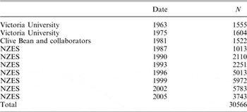
Within each election, weights were applied for age and gender, Maori electorates (oversampled in 1996, 2002 and 2005), university education and vote/non-vote on a registration/enrolment base from census data and official election results. Unweighted sample Ns for each election were as in Table A1.
The Election Studies

There are various sources for further information on the survey data.Footnote 39 Alternative versions of the models were run weighting turnout on an age-eligible basis. Findings were not appreciably different. Alternative versions were also run weighting the Ns of all elections equally. Yet as the inferences to be drawn in the models are individual-level, it was determined to leave the election Ns as in the original Ns for the various studies, remaining as distributed in Table A1. Nor were robust standard errors for clustering applied, for similar reasons. As the datasets were weighted to represent actual turnout patterns at each election, the estimates for election-level variables, the standard errors of which would be adjusted, are not in question. What remains in question is their influence as controls on the estimates of other variables that are subject to sampling error at the individual level.
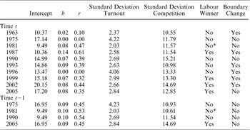
Table A2 reports the results of the constituency regressions discussed in footnote 32. Note that the Maori electorates are excluded as they form a distinct sub-system combining low turnout with low competition until more recent elections under MMP (in particular, 1996 and 2005).
District Competitiveness at times t and t−1 and Turnout Across Various Elections, General Electorates Only

* In 1981, Labour won slightly more votes than National, but fewer seats.
Source: New Zealand elections district level data, http://www.jackvowlesdomain.co.uk/nzelect.html.
Dependent Variable
No Vote = 1, Vote = 0. Voting was validated against the marked rolls for all election studies from 1990 onwards.
Vote Validation
The NZES codes the votes of both respondents and non-respondents from the marked master rolls held in electoral offices around the country. In the checking of the 2008 validation file, to their dismay NZES analysts found more non-voters than the official tables indicated, to an extent well outside the expected sampling error. Further investigation indicated that the number of special voters in the file was too low. Special votes are those cast by voters outside their normal electorates on or before the day of the election. From further checking, it was confirmed that in some electoral offices the information has not been fully transferred to the marked rolls. The numbers involved could be up to 3–4 per cent of enrolled voters in the electorates affected. While this seems small, because the response rates of non-voters are lower than those of voters, on worst case assumptions special voters could make up, on average, as many as 25–30 per cent of respondents coded as non-voters in those electorates where the problem occurs. Investigation of the 2002 and 2005 validation files found similar errors, fortunately to a lesser degree. In the samples, the electoral offices most likely failing to provide a full master roll for inspection can be identified by the extent of their deviation from the official tables. For 2005, seventeen electorates had to be dropped from the sample, and for 2002, thirteen.Footnote 40 While some electorates in which the problem exists may remain in the sample, the damage in terms of miscoding is almost certainly reduced to acceptable limits. The number affected in 2008 is larger, one reason why the 2008 NZES is not available for analysis here. The electorates in which electoral offices failed to complete the master roll had no obvious characteristics, except that in 2005 they included six out of the seven Maori electorates. Alternative models that retained another three of the least biased Maori electorates were no different from those with only one, as reported in the models above. Models were also run on self-reported turnout. These were broadly similar and, where different, the differences were minor and of no theoretical relevance. Self-reported turnout was rejected as an alternative approach because of the small number of non-voters recorded in some of the samples: validation, when accurate, normally approximately doubles the non-voter sample in the NZES.
Independent Variables
Age cohorts and age: Generations are defined from year of birth as explained in the body of the text, and life cycle effects from age at the time of interview.
Country margin: Absolute value of percentage difference between National and Labour vote shares at the election in question (t), and the one before (t−1).
District margin: Absolute value of percentage difference between first and second electorate vote shares in the district in which people at that location would have been voting at the election in question (t) and the one before (t−1).Footnote 41 Where boundary changes took place, codes were available for both new and old electorates, so respondents were classified in terms of experience at that locality of competition at the previous election, rather than, where electoral boundaries changes took place, in terms of the t−1 margin calculated from voting data from the previous election redistributed into the new boundaries. All aggregate-level estimates based on t−1 must, of course, use this method, but that used here is more accurate in terms of reflecting most voters’ actual experiences at the previous election. The exception was 1963, where no 1960 boundary codes were available. Data from the 1960 boundaries for the constituencies in question were used; but, of the four in question, only one was marginally affected by the changes.
SMP: Elections 1993 and before=1, Elections 1996 and after 0.
New voters: Identifies respondents in the various samples eligible to vote in one of their first three elections on grounds of age at the time of the election.
Competition ‘footprints’: (1) The average of absolute percentage differences between the first and second parties nationally over the first three elections for which respondents were eligible to vote, and (2) the average of the averages of absolute percentage differences between first and second parties across all electoral districts over the first three elections for which respondents were eligible to vote.
Average turnout Elections 1–3: Average of age-eligible turnout for the first three elections at which respondents were eligible to vote.
Probability Estimates
Calculations of minimum–maximum probabilities and the data in Figures 3 and 4 used spost’s prchange and prvalue procedures in STATA/IC 10.1.Footnote 42 To estimate age cohort probability effects, all age cohort effects but the one in question were set at 0, and all other variables at the mean. This more accurately estimates the percentage difference against the residual category, where all the cohort variables are 0. All variables, including the cohort variables, were set at means for the calculation of other effects. For the predicted probabilities, the interacting variables were set at 0, or at main effect means, when appropriate.