Introduction

The possible future instability of the West Antarctic ice sheet (WAIS) and its effects on global sea-level rise have been a major focus of Antarctic research for the last several decades. Field and remotely sensed data revealed a complex structure in the WAIS drainage system (Reference JoughinJoughinand others, 1999) and enabled us to better elucidate the basal processes that permit fast ice-stream motion under low driving stresses (Reference Alley, Blankenship, Bentley and RooneyAlley and others, 1987a,Reference Alley, Blankenship, Rooney and Bentleyb, Reference Alley, Blankenship, Rooney and Bentley1989; Reference Blankenship, Bentley, Rooney and AlleyBlankenship and others, 1987; Reference Engelhardt, Humphrey, Kamb and FahnestockEngelhardt and others, 1990; Reference Engelhardt and KambEngelhardt and Kamb, 1997; Reference Anandakrishnan, Blankenship, Alley and StoffaAnandakrishnan and others, 1998; Reference BellBell and others, 1998 ;Reference Tulaczyk, Kamb, Scherer and EngelhardtTulaczykandothers,1998, Reference Tulaczyk, Kamb and Engelhardt2000a,Reference Tulaczyk, Kamb and Engelhardtb; Reference Kamb, Alley and BindschadlerKamb, 2001). High basal water pressures and a layer of weak till with a large porosity seem to play the key role in facilitating the fast ice streaming inWest Antarctica (Reference Engelhardt, Humphrey, Kamb and FahnestockEngelhardt and others, 1990; Reference Harrison, Echelmeyer and EngelhardtHarrison and others, 1993, Reference Harrison, Echelmeyer and Larsen1998; Reference Echelmeyer, Harrison, Larsen and MitchellEchelmeyer and others, 1994; Reference Engelhardt and KambEngelhardt and Kamb, 1997; Reference Tulaczyk, Kamb, Scherer and EngelhardtTulaczyk and others, 1998, Reference Tulaczyk, Kamb and Engelhardt2000a, Reference Tulaczyk, Kamb and Engelhardtb; Reference Kamb, Alley and BindschadlerKamb, 2001). It is therefore clear that the spatial and temporal availability of basal water has to be incorporated into models simulating the present and future behavior of the WAIS (see, e.g., Reference Budd, Jenssen and SmithBudd and others, 1984,Reference Budd, Coutts and Warner1998; Reference MacAyealMacAyeal, 1993; Reference Fastook and PrenticeFastook and Prentice, 1994; Reference PaynePayne, 1998, Reference Payne1999; Reference Hulbe and MacAyealHulbe and MacAyeal,1999; Reference Hulbe, Joughin, Morse and BindschadlerHulbe and others, 2000; Reference RaymondRaymond, 2000).

Borehole observations in the interior of the WAIS (Reference RobinRobin, 1983) and in the Siple Coast ice streams (Reference Engelhardt, Humphrey, Kamb and FahnestockEngelhardt and others, 1990) revealed a wet bed with ice at, or close to, its pressure-melting temperature. Recent drilling at the UpC “sticky spot” revealed a 12–25m thick sediment-laden, bubble-free layer of basal ice (personal communication from H. Engelhardt, California Institute of Technology (Caltech) field season 2000/01), henceforth referred to as the basal ice layer. The appearance and composition of the layer are consistent with its origin by basal freeze-on (Vogel and others, unpublished stable-isotope data). The presence of this basal ice layer indicates that basal freeze-on, rather than melting, prevailed for at least several thousand years, upstream of the UpC area. Lacking direct observations from ice-stream tributaries, which channel ice toward the UpCarea,weusedathermodynamical numerical model to assess their basal energy balance. Our goal is to test whether accretion of the thick basal ice layers could have occurred as the ice, found now in the UpC area, traveled through the tributaries of Ice Stream C.

Ice Stream C Catchment Areas

Ice Stream C (Fig. 1) is located in the central part of the Siple Coast. The Ice Stream C trunk is separated from its southern neighbor Whillans Ice Stream (formerly Ice Stream B) by the interstream ridge B/C, and from its northern neighbor Ice Stream D by Siple Dome. Having two main tributaries, Ice Stream C draws its ice from the northeastern WAIS divide common with the Amundsen Pine Island Glacier catchment area and from the southeastern WAIS divide common with the Weddell Sea catchment area. Originating in the Byrd Subglacial Basin (BSB; up to 2500m below sea level), the northern tributary draws its ice from the more northeasterly ice divide. Convergingfrom the surrounding mountain blocks into the BSB, the ice reaches a maximum thickness of >4000m, before it speeds up and emerges following the Bentley Subglacial Trench (BST) towards the now stopped trunk of Ice Stream C. The southern tributary originates from the southeastern divide in the Whitmore Mountains. Drawing its ice from the topographically higher Whitmore mountain block, the ice thickness of its sub-tributaries is thinner (∼2000 m) and increases only when the ice is crossing a trench connecting a gap between the Whitmore mountain block and the Transantarctic Mountains with the emerging BST.

Fig. 1.

Bed topography (a), surface elevation (b) and surface velocity field (c) in the catchment area of Ice Stream C. Also shown are the location of places referred to in the text and the location of the profile lines (gray lines) used in our basal energy model. The insert in (c) shows the approximate location of the graphs in Antarctica.

In our model, we consider two different flowlines for each tributary (Fig. 1; see Fig. 2 for details). For the northern tributary, one flowline (CN-NW) originates close to the junction of the Amundsen Sea embayment, the Weddell Sea and Ross Sea catchment areas. The other flowline (CN-S) initiates at the southeastern divide with the Weddell Sea catchment area, crossing the Byrd Plateau and flowing through a smaller sub-tributary into the main tributary. Both flowlines of the southern Ice Stream C Tributary (CS) originate in the Whitmore Mountains. The flow of the southern flowline (CS-S) recently got diverted towards Whillans Ice Stream. The northern flowline (CS-N) flows in its lower part, separated by a small ridge almost parallel to the southern flowline of the northern tributary. In the UpC area, flowline CN-NW passes the sticky spot in the north, while all other flowlines pass in the south.

Fig. 2.

Profiles of the four simulated flowlines converging toward the UpC area of Ice Stream C: (a) CN-NW; (b) CN-S; (c) CS-N; and (d) CS-S.The upper diagram of each flowline shows surface and bed elevation, while the lower diagram shows the ice velocity used in the model and the observed ice velocity (dotted where it differs from the model velocity). In the upper part of the ice stream we have arbitrarily adjusted ice velocities to account for the faster ice flow expected prior to the shut-down of Ice Stream C.

The Basal Energy-Balance Model

We calculate the basal energy balance taking into account the geothermal flux (GT), the basal shear heating (SH), the heat (C) conducted through the ice away from the bed and the heat (M) used or released by either melting or freezing at the ice base:

The melting or freezing rate (m) is the quotient of the energy balance and the latent heat of fusion (L) and density (p),

The basal shear heating is the product of the basal shear stresses (τ_b ) and the basal ice velocity (ub), while the heat conduction away from the bed is determined by the product of the basal temperature gradient (/3_b) and the thermal conductivity of ice (K).

To obtain the basal temperature gradient, we use a numerical thermodynamical flowline model to model the temperature profile in the ice. The model includes heat conduction, vertical and horizontal advection and calculates the temperature profile in the ice. The temperature is calculated at 21 vertical nodes, repeated at 5 km horizontal intervals along the flowline, which is also the horizontal spacing for our basal energy-balance calculations.

As no data about basal conditions beneath ice-stream tributaries are available, we assume in the model that basal conditions in the ice-stream tributaries are similar to those in ice-stream trunks. Water is available for freeze-on at all times at the ice base. Basal temperatures are everywhere at the pressure-melting point (PMP; see Reference PatersonPaterson, 1994, p.212, for PMP calculation). Independent of the individual driving stress, basal shear stresses are taken to be low everywhere, between 1 and 10 kPa (Reference Tulaczyk, Kamb and EngelhardtTulaczyk and others, 2000a; Reference Kamb, Alley and BindschadlerKamb, 2001). In the model, we use a geothermal flux of 70 mW m2. H. Engelhardt (personal communication, 2002) calculated this value using the temperature profile of Siple Dome. This is the only geothermal flux calculation in West Antarctica using a continuous temperature profile. Avoiding speculation about a possible distribution of the geothermal flux underneath the WAIS, we assume this value to be valid along all flowlines. The usage of a higher (lower) value would increase (decrease) basal melting and decrease (increase) basal freezing, but would not change the overall pattern of basal melting beneath the thick ice in the WAIS interior, and freezing in the shallower parts of the WAIS towards the ice streams.

Further on, we assume that basal sliding is the dominant part of ice movement (Reference Engelhardt and KambEngelhardt and Kamb, 1998; Reference Kamb, Alley and BindschadlerKamb, 2001), allowing us to substitute the surface velocity (us) for the basal velocity in Equation (3) and to neglect internal deformation in the temperature model. Therefore we calculate temperature changes at a point within the ice sheet from the vertical heat conduction through the ice and the horizontal and vertical advection of heat (for more detailed discussion of Equation (5) and the effect of general assumptions, see, e.g., Reference RobinRobin, 1983; Reference PatersonPaterson, 1994; Reference Van der VeenVan der Veen, 1999).

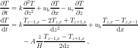
where k is thermal diffusivity (37.2 m² a–¹ at –1°C; Reference HookeHooke, 1998), uh is horizontal velocity (surface velocity), uv = azh-1 is vertical velocity, a is accumulation rate, z is height over the bed, h is ice thickness, ti j is temperature at depth i and location j, and t is time.

In several model runs, we have implemented a quadratic form of the parameterization of vertical ice velocity near the ice divide (Reference PatersonPaterson 1994, p. 220) and have verified that the exact choice of parameterization has negligible effect on our calculations of basal freezing/melting.

We used an atmospheric lapse rate of 0.002 Km – ¹ to calculate the surface temperature distribution by assuming that they are linearly dependent on surface elevation. This value differs from the typical range of atmospheric lapse rates (0.006–0.010 Km–¹ ) . It was calculated using modern 10 m temperatures at Byrd Station (–28°C at 1530 m a.s.l.; Reference RobinRobin, 1983) and Ice Stream C (–26°C at 500 m a.s.l.; Reference Kamb, Alley and BindschadlerKamb, 2001; personal communication from H. Engelhardt, 2001). I n analogy with surface temperature changes, we also parameterized spatial variation in accumulation rates along the simulated flowlines with surface elevation by using a linear fit to modern accumulation data (Reference Giovinetto, Waters and BentleyGiovinetto and others, 1990; Reference Giovinetto and ZwallyGiovinetto and Zwally 2000).

Surface and bed geometry were prescribed in our model using elevation and ice thickness from the BEDMAP dataset (Reference Lythe and VaughanLythe and others, 2001), which was resampled to match the velocity dataset (Reference JoughinJoughin and others, 1999). As the surface velocity field in the tributaries is close to the balance velocity, we assume the velocity field to be constant over time. Where Reference Shabtaie and BentleyShabtaie and Bentley (1987) had mapped the buried shear margin of Ice Stream C, we gradually adjusted the velocity to 100ma–¹ as a transition to the faster ice-stream flow, assuming that the currently lower flow velocities are a result of the Ice Stream C stoppage and that flow in the past was similar to the balance velocity (Reference Bamber, Vaughan and JoughinBamber and others, 2000). After initializing the model over 50 kyr with modern-day surface temperatures, accumulation rates, ice velocities and ice-thickness values, we ran the model over a complete glacial– interglacialcycle from 125 kyr BP to today usingatime-step of 10 model years. During the simulated glacial–interglacial cycle, we adjusted for temperature and accumulation changes (Fig.3a and b) using the Vostok ice-core record (Reference PetitPetit and others, 1999).We smoothed the temperature and accumulation record using a 1000 year moving average. We also varied ice-surface elevation (Fig. 3c) using the WAIS elevation history estimated by Reference Jenssen and RobinJenssen (1983) and Reference Steig, Alley and BindschadlerSteig and others (2001). As the values given by Reference Jenssen and RobinJenssen (1983) overestimate elevation changes, we adjust his numbers downward for the time period from 11500 years BP to 45000 years BP, using the difference between his value at 11500 years BP and the value for the same time given by Reference Steig, Alley and BindschadlerSteig and others (2001). For simplicity, we assume uniform elevation changes along all flow-lines and do not consider different thickness changes in different parts along the flowline (see, e.g., Reference Steig, Alley and BindschadlerSteig and others, 2001; Waddington and others, http://igloo.gsfc.nasa.gov/wais/abstracts01/Waddington.html ). If we were to do so, we would have to engage in speculation since there are no data that could be used to infer ice-thickness histories in different parts of our flowlines. Also several model runs have showed that possibly larger ice-thickness changes in the UpC area or ice-stream trunks (Waddington and others, http://igloo.gsfc.nasa.gov/wais/abstracts01/Waddington.html) have negligible influence on the basal ice production upstream of this location. This also can be easily illustrated, as the ice influenced by a thickened Last Glacial Maximum (LGM) UpC area has moved further downstream and the ice currently present in the UpC area has moved into the UpC area from further upstream.

Fig. 3.

Graphs showing the history of (a) surface temperature, (b) surface accumulation rate, and (c) WAIS elevation changes over the last 125 000 years. Surface-temperature changes and parameterized accumulation rates are based on the Vostok ice-core record (Reference PetitPetit and others, 1999). Ice surface-elevation changes are based on our reinterpretation of the reconstructions by Reference Jenssen and RobinJenssen (1983) and Reference Steig, Alley and BindschadlerSteig and others (2001).

Results

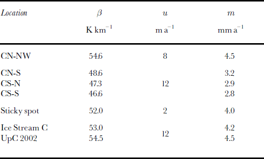
Figure 4 compares the modeled present-day temperature profile at the UpC sticky spot (around km 600 in the profile lines) with the measured one (personal communication from H. Engelhardt, 2001). Along the flowline, the simulated basal temperature gradient ranges from 30 to 60Kkm– 1 (Figs 5a and g and 6a and g). The flowlines passing south of the sticky spot show a similar basal temperature gradient of 47.5K km– 1 (±1Kkm–1) (see Table 1). This is 6.2Kkm–1 lower than the measured temperature gradients in the southern Ice Stream C branch. The basal temperature gradient for the northern Ice Stream C branch at the sticky spot (profile line CN-NW) is 54.6 K km–¹: similar in magnitude to, yet 7.1 K k m ^{– 1} higher than, those for the southern Ice Stream C branch. Unfortunately, no measured temperature profile is available for the northern Ice Stream C branch, so we focus our comparison of basal ice accumulation below on the profile lines passing through the southern ice-stream branch, in which the discovery was made. In the southern ice-stream branch at the UpC location, the estimated modern freeze-on rate is 4.2 ± 0.2 mm a–¹ (Table 1; Reference Kamb, Alley and BindschadlerKamb, 2001), - 1 3 mm a ¹ higher than the modeled rates. Hence the model underestimates basal freeze-on rates at this location by - 3 0 % .

Fig. 4.

Measured temperature profile at upc camp (solid line; courtesy of h. engelhardt); the temperature profiles of profile lines cn-s, cs-nand css (dashed lines), originating on the byrd plateau and passing the upc sticky spot in the south; and the temperature profile of profile line cn-nw (dotted line), which emerges from the bsb and passes the upc sticky spot in the north. the basal temperature gradient of the three dashed lines is lower than the measured one, while the cn-nwprofile has a higher temperature gradient.

Fig. 5.

Results for the profile lines CN-NW (a–f) and CN-S (g–l) of the northern Ice Stream C tributaries. (a, g) Current (solid line) and early-Holocene (10 kyr; dashed line) basal temperature gradient; (b, c, h, i) basal melt and freezing cumulative along the flowline starting at the ice divide, using 1kPa (solid line) and10 kPa (dashed line) as basal shear stress; (d, j) basal freezing rates along flowline using 1kPa (solid line) and 10 kPa (dashed line) as basal shear stress; (e, k) basal freezing rates for present day (1kPa; solid line) and early Holocene (10 kyr;1kPa dashed line, 10 kPa dash-dotted line); (f, l) time evolved since ice started to move away from ice divide.

Fig. 6.

Results for the profile lines CS-N (a–f) and CS-S (g–l) of the northern Ice Stream C tributaries. (a, g) current (solid line) and early-Holocene (10 kyr; dashed line) basal temperature gradient; (b, c, h, i) basal melt and freezing cumulative along theflowline starting at the ice divide, using1kPa (solid line) and 10 kPa (dashed line) asbasal shear stress; (d, j) basal freezing rates along flowline using 1kPa (solid line) and10 kPa (dashed line) as basal shear stress; (e, k) basal freezing rates for present day (1kPa; solid line) and early Holocene (10 kyr;1kPa dashed line, 10 kPa dash-dotted line); (f, l) time evolved since ice started to move away from ice divide.

Table 1.

basal temperature gradient ((3), ice velocities (u) and basalfreeze-onrates(m)at1kpa

Along the flowlines, the threshold basal temperature gradient for basal freezing varies, dependent on ice velocity, from 33 to 35 K km–¹ (33 to 45 K km–¹ for r_b = 10 kPa), for a basal shear stress of 1 kPa. Comparing the obtained melting rates with the freezing rates shows a distinct difference between the northern and southern tributaries (Table 2; Figs 5b–e and h–k and 6b–e and h–k). Basal melting is high underneath the thick ice of the WAIS interior (over the first 200–300km of the flowlines), while basal freezing is dominant in the thinner parts of the tributaries closer to the UpC area. Basal melting is particularly high in the BSB (km 50– 200, flowline CN-NW, Fig. 5a–f) and starts to decrease where ice emerges from the BSB. Further thinning of ice in the BST leads to a steepening of the basal temperature gradient and to basal freezing, allowing the accretion of up to 17 mofbasaliceinthemodel.

Table 2.

Modeled basal melting andfreezing (m)beneath Stream C tributaries

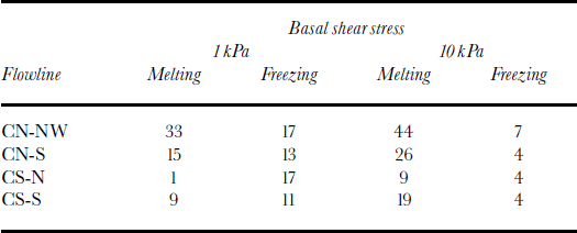
Basal freezing close to the ice divide in the tributaries originating on the Byrd Plateau (southern tributaries and CN-S; see Fig. 1) possibly indicates that the ice sheet is frozen to its bed and that heat used in the model to melt ice at the base of the ice sheet further downstream will actually be used to warm the basal ice until the PMP is reached.

Taking into account the possibility of a frozen bed on the Byrd Plateau, we consider only the last 300–400km of each flowline while estimating the thickness of basal ice at the UpC sticky spot (100 km from the end of each flowline). Considering the underestimation of basal freeze-on rates (∼1.3 mm a–¹ or ∼ 3 0 %) i n the southern ice-stream branch at the UpC sticky spot, the modeled basal ice thickness (6– 13 m) at the UpC sticky spot (Table 3) is similar in magnitude to the observed basal ice thickness of 10–25 m. With a higher basal shear stress of 10 kPa, the model still obtains a basal ice thickness of up to 3 m at this location; while with a basal shear stress of 22 kPa no basal ice is obtained. A further increase in basal shear stress to 70 kPa leads to 4 150 m of basal melt.

Table 3.

Modeled basal ice thickness (m) at the UpC spot (km 600)

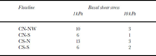
These calculations illustrate the sensitivity of predicted basal ice thickness at UpC to the assumed magnitude of Ice basal shear stress. In reality, there is likely to be a spatial variability in the basal shear stress, but, with no firm observational constraints available, we opted for a simple assumption of a constant basal shear stress along all of the considered flowlines. In the case of advection of the basal ice layer from upstream (see third paragraph of Discussion below), these sensitivity analyses also show that moderate basal shear stresses (∼20 kPa) have to be present in the ice-stream tributaries in order to preserve such a feature.

Discussion

If our conceptual picture of basal ice formation by basal freeze-on upstream of UpC is correct, we have to contend with the fact that the model predicts that basal melting and freezing occur in spatially separated areas. In order to sustain the basal freeze-on expected from our model results, either water is transported between these two areas, or basal water, locally stored in the system, from earlier melt events is used in the freeze-on process, or both. Although we do not know precisely what form the latter water storage of subglacial water would take (subglacial lakes?), one can observe that the basal temperature gradients in our model (Figs 5a and g and 6a and g; solid line present day, dashed line 10 kyr BP) are consistently smaller during the late LGM and early Holocene than today. This model prediction suggests the possibility of more widespread melting and higher melting rates during this time. The ultimate physical reason for the lower late-LGM and early-Holocene basal temperature gradient is the assumed greater ice thickness at that time (Reference Steig, Alley and BindschadlerSteig and others, 2001). We speculate that this higher basal water production may have also helped to lubricate the base of the ice sheet and promote its rapid Holocene decay (Reference Conway, Hall, Denton, Gades and WaddingtonConway and others, 1999).

One can use our results to consider a regional basal water balance over roughly the area of the BSB and other similarly deep parts of the WAIS interior (Reference Parizek, Alley, Anandakrishnan and ConwayParizek and others, 2002) as well as the shallower part of the Ice Stream C tributaries. This regional balance between basal melting and basal freezing for the Ice Stream C tributaries (see Table 2) may have shifted from being a source of basal water in the early Holocene to a sink in modern times. Reduction in the amount of water stored in the subglacial hydrological system could increase basal resistance (Reference Tulaczyk, Kamb and EngelhardtTulaczyk and others, 2000b), which would be consistent with present-day force-budget calculations (Reference Joughin, Tulaczyk, Bindschadler and PriceJoughin and others, 2002) and the observed slow-down of Whillans Ice Stream (Reference Joughin, Tulaczyk, Bindschadler and PriceJoughin and others, 2002) as well as the shut-down of Ice Stream C (Reference Anandakrishnan and AlleyAnandakrishnan and Alley, 1997). It is important to note, however, that the conjectured persistence of high basal shear stresses (∼70 kPa; Reference Joughin, Tulaczyk, Bindschadler and PriceJoughin and others, 2002) in the past along the entire flowline would have caused extensive basal melting (150m in our model), making basal freeze-on an unlikely explanation for the observed basal ice layer at the UpC sticky spot.

The model currently does not take into account the possibility of a frozen bed in parts of the WAIS interior and also does not treat explicitly latent-heat transport through basal water drainage. Further uncertainties of the model result from unknown changes in the ice-flow history and in the WAIS elevation history. Given the simplifying assumptions that went into the construction of our model, we cannot use the model results to claim that the debris-laden basal ice layer found in boreholes drilled in the UpC area of Ice Stream C must have formed by freeze-on beneath the tributaries of this ice stream. We can only say that such genesis of the basal layer is admissible, given a restrictive condition of very low basal shear stresses everywhere beneath simulated flowlines. An alternative explanation for the origin of this layer is suggested by Reference Christoffersen and TulaczykChristoffersen and Tulaczyk (2003), who show that ∼20m of frozen-on basal ice may have formed beneath interstream ridges as a result of the cooling trend during the last glacial cycle. Reference Kamb, Alley and BindschadlerKamb’s (2001) analysis of borehole data from interstream ridges indicates that they may be underlain by thick (up to 10–41m) debris-laden basal ice layers. An ice core recovered from Byrd Station contained ∼ 5 m of debris-laden basal ice. Hence, an alternative explanation for the basal layer at UpC is that it represents a feature formed in slow-moving ice (outside of ice-stream tributaries), which was then incorporated into the tributaries of Ice Stream C and advected to the UpC area.

Future field research, in particular the drilling of boreholes to examine ice-stream tributary beds in the WAIS interior and additional temperature measurements, seems necessary for constraining basal water production rates and basal water distribution beneath ice-stream tributaries and the WAIS interior. Improved, physically based parameterizations of these processes are needed to accurately model the past and future behavior of the WAIS (Reference Steig, Alley and BindschadlerSteig and others, 2001) and to assess the possible threat of a rapid sea-level rise caused by a rapid disintegration of the WAIS (Reference MercerMercer,1978; Reference Scherer, Aldahan, Tulaczyk, Possnert, Engelhardt and KambScherer and others, 1998).

Conclusions

Our numerical model applied to three different flowlines converging near the UpC sticky spot shows that the 10–25mthick basal ice layer observed in the UpC area may have formed by basal freeze-on occurring beneath ice-stream tributaries. Admittedly, the model can produce a sufficient amount of basal ice only if we assume that beds of tributaries are as weak as the till beds found beneath ice-stream trunks (1– 10 kPa). In our model, basal melting was highest during the LGM, due to a thickened ice sheet. According to the model, basal melting rates in the WAIS interior peaked around 15 kyr BP. This increase in availability of basal water could have played a role in initiating the rapid Holocene decay of the WAIS. A subsequent increase in basal freeze-on rates related to ice thinning might have shifted the basal energy balance towards freezing. The latter process may have gradually reduced the amount of basal water in the subglacial system over the course of the Holocene. A reduction of basal water availability can lead to an increase in basal resistance to fast ice motion and should be considered as one possibility for the recent shut-down of Ice Stream C and the current slow-down of Whillans Ice Stream. These conjectures, however, need to be verified by field observations.