2. Governing equation

In Cartesian coordinates, the equation governing the streamfunction, $\psi ( x,z),$ for inviscid, two-dimensional, linear internal wave propagation of frequency $\omega$ in a uniformly stratified fluid (constant buoyancy frequency, $N$, and Coriolis frequency, $f_{0}< N)$ is the hyperbolic-in-space Poincaré or Poincaré–Sobolev equation

(2.1)\begin{equation} \frac{1}{c^{2}}\frac{\partial^{2}\psi}{\partial x^{2}}-\frac{\partial^{2}\psi }{\partial z^{2}}=0,\quad c^{2}=\frac{\omega^{2}-f_{0}^{2}}{N^{2}-\omega^{2} }>0,\quad c>0, \end{equation}

in a channel of depth $h( x)$ as here, or in an infinitely deep ocean, $-\infty < z\leq h$. A factor $\exp ( -{\rm i}\omega t)$ is implicit. The velocity field, $\boldsymbol {u}=(u,w),$

(2.2a,b)\begin{equation} u=\frac{\partial\psi}{\partial z}, \quad w={-}\frac{\partial\psi}{\partial x}, \end{equation}

is subject to a top boundary condition of $w=0$ and a bottom boundary condition of ${\boldsymbol {u}\boldsymbol{\cdot }\boldsymbol {\nabla }} {(h-z)}=0,$ i.e. no normal flow. If $c^{2}<0$, that is, $\omega ^{2}>N^{2}$ or $\omega ^{2}< f_{0}^{2}$, the nature of the equation changes from hyperbolic to elliptic. This latter regime, particularly important for diurnal and longer period tidal forcing poleward of approximately $30^{\circ }$ latitude, is of considerable oceanographic interest, but is not discussed here. When $\omega ^{2}/N^{2}\rightarrow 0,$ the system is hydrostatic. Llewellyn Smith & Young (Reference Llewellyn Smith and Young2002) described the important role of a finite, reflective, upper boundary relative to an infinitely deep ocean.

Equation (2.1) has been written so that, if $t$ (time) is substituted for $x,$ the equation has the same form as an ordinary one-dimensional wave equation with wave speed $c.$ In such problems, a boundary that moves faster than $c$ would generate a shock, or be physically impossible if $c$ is the speed of light (see, e.g. Balazs Reference Balazs1961 or Greenspan Reference Greenspan1963). These problems require causality in the $x,t$ domain, but no such causality is required in $x,z$ where information can flow ‘backwards’ in $x.$ As is well known, the internal wave problem can be divided into regimes according to the topographic slope. Here, we consider the regime with slopes $\gamma$ that are sufficiently shallow ($\gamma < c$) so that no non-causal characteristics are generated by reflection of causal characteristics off the topography. Such slopes are labelled ‘transmissive’ or ‘sub-critical’ meaning that energy (information) is not returned in the direction in $x$ from which the disturbance originated. By contrast, when slopes are sufficiently large $\ (\gamma >c),$ non-causal characteristics can exist; these slopes are ‘reflective’ or ‘super-critical’. Poincaré (Reference Poincaré1885) discussed the corresponding spatially hyperbolic equation for the interior of an unstratified, $N=0,$ but strongly rotating, fluid container. As a ‘critical’ slope, $\gamma =c,$ is approached, the characteristic curves become tangent to the boundary, and solution infinities are generated. What follows is restricted to the transmissive, subcritical, case.

From here, the notation differs slightly from that in M11: the $z$-coordinate origin is taken at constant reference depth, $h,$ so that the upper rigid lid is at $z=h.$ The most natural spatial scale comes from the water depth, so that a non-dimensional vertical coordinate, $z^{*}$ is defined as $z=hz^{*}$ and the non-dimensional horizontal coordinate is defined as $x=hx^{*}/c.$ The upper lid is at $z^{*}=1$ and the disturbance to the seafloor about $z=0$ is $z=h_{1}( x/h)$ or $z^{\ast } =h_{1}( {x^{\ast }/c}) /h\ll 1.$ Equation (2.1) becomes

(2.3)\begin{equation} \frac{\partial^{2}\psi^{{\ast}}}{c^{{}^{*}2}\partial x^{{}^{*}2}} -\frac{\partial^{2}\psi^{{\ast}}}{\partial z^{{}^{*}2}}=0,\quad c^{*}=1;\end{equation}

where $c^{*}$ is retained as a mnemonic device. With a flat bottom, the dimensional forced oscillatory solution to (2.1) consists of a uniform horizontal flow

(2.4)\begin{equation} \psi_{0}( z) =Uz,\end{equation}

and non-dimensional $\psi$ is defined from $\psi =(Uh)\psi ^{*}.$ Flow is left to right when $U>0,$ although oscillating in direction with $t$. Choose $U=1.$

At this point, the $*$ will be dropped, all variables being non-dimensional. The role of $c$ is as a reminder that the horizontal scale will change with the frequency of oscillation. With a flat bottom, in addition to $\psi _{0},$ an infinite set of internal wave modes exists

(2.5)\begin{equation} \psi_{iw}=\sum_{m={-}\infty}^{\infty}A_{m}\, {\rm e}^{{\rm \pi} imcx}\sin( m{\rm \pi} z), \end{equation}

all satisfying the two Dirichlet boundary conditions $\psi ( z=0,z=1) =0,$ and which radiate to and from infinity in $\pm x.$ Periodicity in $cx$ is $2.$ For these vertically standing modes, zonal phase and group velocities are in the same direction.

Assume now that a non-zero value of $\psi _{0}=z$ is imposed in the channel with a perturbation $h_{1}(cx)$ to the bottom boundary, so that the non-dimensional bottom boundary condition is linearized about $z=0$ with $U=1$

(2.6)\begin{equation} ( u,w) \boldsymbol{\cdot}\boldsymbol{\nabla} {(h-z)}=\frac{\partial h_{1}}{\partial (cx)}-w( z=0) =0.\end{equation}

Balmforth, Ierley & Young (Reference Balmforth, Ierley and Young2002), Pétrélis, Llewellyn Smith & Young (Reference Pétrélis, Llewellyn Smith and Young2006) and a number of other authors provided examples of what is considered the ‘forward’ or ‘direct’ problem for $\psi$, given $h_{1}(cx).$ When $\partial h_{1}(cx) /\partial (cx)<1,$ the slope is subcritical. In an infinite channel as discussed here, radiation conditions must usually be imposed as $|cx|\rightarrow \infty.$ (A finite amplitude case is considered briefly at the end.)

3. Simplified solution

Consider, in non-dimensional space, subcritical, transmissive topography, $h_{1}(cx),$ with the boundary condition linearized about $z=0$. Let

(3.1)\begin{equation} \psi=f(cx-z+\alpha_{1}) +g(cx+z+\alpha_{2}), \end{equation}

where $f,g$ are arbitrary, but twice differentiable, solutions to (2.3), and where $\alpha _{i}$ are constants. On $z=1,$ $f(cx-1+\alpha _{1}) =-g(cx+1+\alpha _{2}),$ and choosing $\alpha _{1}=1,$ $\alpha _{2}=-1$ (in effect, using the method of images), $g( q) =-f( q).$ Then

(3.2)\begin{equation} \psi(cx,z) =f(cx-z+1) -f(cx+z-1),\quad -\infty\leq x\leq\infty, \end{equation}

satisfying the upper boundary condition, $\psi ( z=1) =0$ (see Manton & Mysak Reference Manton and Mysak1971; Bühler & Holmes-Cerfon Reference Bühler and Holmes-Cerfon2011).

If the difference in (3.2) is non-zero only inside some interval $P$, effectively vanishing outside $x\in P,$ then no far-field radiation will be generated. Following mathematical practice, functions with that confined support will be called ‘rapidly decreasing functions’ (RDF); see Cheney (Reference Cheney2001). If no far-field disturbance occurs, then radiation conditions (RC) become irrelevant.

The perturbation vertical velocity is

(3.3)\begin{equation} w(cx,z) ={-}\frac{\partial\psi}{\partial(cx) }={-}f^{\prime}(cx-z+1) +f^{\prime}(cx+z-1), \end{equation}

and setting

(3.4)\begin{equation} w(cx,0) ={-}f^{\prime}(cx+1) +f^{\prime} (cx-1)=\frac{\partial h_{1}}{\partial(cx) }, \end{equation}

or

(3.5)\begin{equation} -f(cx+1)+f(cx-1)=h_{1}(cx)+H, \end{equation}

with $H$ arbitrary and set to zero. Here, $h_{1}(cx)$ will be RDF if the difference in (3.5) is RDF even if $f(cx)$ is not itself RDF. Any $f(cx)$ of period $2$ (the usual non-RDF (2.5) flat-bottom radiating free modes) can be added to the solution $f,$ without necessitating a change in $h_{1}.$

Note that non-radiating examples are easy to come by: we may freely specify $f$ a function of rapid decrease, and then simply set

(3.6)\begin{equation} h_1(cx)= f(cx-1)-f(cx+1), \end{equation}

to obtain the topography, and recover $\psi$ from (3.2), which inherits rapid decay (in $x$) from $f.$ An explicit example of this construction is as follows:

Let

(3.7)$$\begin{gather} f(cx) =\varepsilon\operatorname{sech}({\rm \pi} cx), \end{gather}$$

(3.8)$$\begin{gather}f^{\prime}(cx) ={-}{\rm \pi}\varepsilon\operatorname{sech}( {\rm \pi}cx) \tanh( c{\rm \pi} x), \end{gather}$$

then

(3.9)\begin{equation} \psi=\varepsilon[ \operatorname{sech}{\rm \pi}(cx-z+1)-\operatorname{sech} {\rm \pi}(cx+z-1)], \end{equation}

which is exponentially confined to the topography with no radiation. Here and elsewhere, $\varepsilon$ is a small parameter. Also

(3.10)$$\begin{gather} w={\rm \pi}\varepsilon[ \operatorname{sech}{\rm \pi}(cx-z+1) \tanh {\rm \pi}(cx-z+1) -\operatorname{sech}{\rm \pi}(cx+z-1) \tanh{\rm \pi}(cx+z-1)], \end{gather}$$

(3.11)$$\begin{gather}h_{1}(cx) =\varepsilon[ -\operatorname{sech}({\rm \pi}(cx+1) )+\operatorname{sech}{\rm \pi}(cx-1)], \end{gather}$$

(3.12)$$\begin{gather}h_{1}^{\prime}(cx) ={\rm \pi}\varepsilon[ \operatorname{sech}( {\rm \pi}(cx+1) ) \tanh( {\rm \pi}(cx+1) ) -\operatorname{sech}{\rm \pi}(cx-1) \tanh{\rm \pi}(cx-1) ], \end{gather}$$

is the corresponding topography determined inversely from the solution. The flow and topography for $\varepsilon =0.1$ can be seen in figures 1 and 2 where $h_{1}(cx)$ becomes constant and hence non-radiating.

Figure 1.

Topography (upper panel) and its derivative (dashed line) and the solution (lower panel), $\psi ( x,z)$ in (3.9). Here, $c=1,\varepsilon =0.1.$ No far-field radiation occurs.

Figure 2.

Value of $w( x,z=1/2) =-\partial \psi /\partial x,$ for the double $\operatorname {sech}$ bottom profile.

This ‘non-converting’ or ‘non-radiating’ field was called, in M11, the ‘non-hydrostatic barotropic’ flow. But given the numerous conflicting definitions of ‘barotropic’ in the literature, the terminology is avoided here.

In an oceanographic context, the possible existence of such trapped solutions implies a relatively high shear, and hence strong mixing over topographic features. A far-field measurement of the resulting disturbance would vanish, and no information about the shear would be recoverable directly. (Indirect estimates might be possible through the influence of a strong mixing region on the larger-scale flow field.)

4. Some generalization

The label ‘compact support’ implies a function that is identically zero outside an interval $P.$ Such functions $f,$ or topographies, $h_{1}$, do not exist in the real world unless entire ocean basins are considered, and then lateral boundary conditions intrude. Within the class of RDF, ‘bump’ functions are identically zero outside $P,$ and the ‘Schwartz functions’ (‘good’ functions in the terminology of Lighthill (Reference Lighthill1958) and others) are RDF but are also perfectly smooth (infinitely differentiable), with all derivatives also enjoying rapid decay. For what follows, the most important characteristic of Schwartz functions in wavenumber space is that their Fourier transforms are also Schwartz functions. Rapidity of decay is still subject to the uncertainty principle, however, so that bandwidth in one domain is inversely proportional to that in the other.

To the extent that the wavenumber decay is proportional to a power of $k^{-p},$ and viscous decay is proportional of $\nabla ^{2}( u,v,w)$, the value $p$ will determine the relative importance of high-wavenumber dissipation. Thus if $p=2,$ dissipation is uniform in $k;$ and larger values of $p$ will tend to minimize high-wavenumber contributions to dissipation.

As above, given $f(cx)$ from a known $\psi (cx,z)$, then in a simple formal inverse problem, $h_{1}(cx)$ is easily determined: the solution is known, and the boundary shape, $h_{1}(cx),$ is found by subtraction. The Appendix briefly summarizes a situation of practical observations, including noise.

Here, the conventional wave generation ‘forward’ problem: for given $h_{1}(cx)$, find $f^{\prime }(cx),$ is more interesting, both with and without an RDF requirement. Equation (3.5) is an innocuous-seeming functional equation examined by Manton & Mysak (Reference Manton and Mysak1971) and more recently by Beckebanze & Keady (Reference Beckebanze and Keady2016), the latter emphasizing closed containers without RC (Aczél (Reference Aczél1966) is a general discussion of functional equations). Hazewinkel et al. (Reference Hazewinkel, Tsimitri, Maas and Dalziel2010) discuss the application of wave attractors to similar problems. Colin De Verdiere & Saint–Raymond (Reference Colin De Verdiere and Saint–Raymond2020) and Dyatlov & Zworski (Reference Dyatlov and Zworski2019) have recently revisited the analysis of attractors via methods of microlocal analysis. If the RDF requirement is abandoned, (3.5) provides a general relationship between any perturbation topography and a function $f$, but only insofar as RC are satisfied – and which is not so easily accomplished in general. On the other hand, if $\psi$ has compact support, RC are irrelevant.

4.1. Functional equation by operator inversion

As a linear inverse model, (3.5) is a very simple one for determining $h_{1}(cx)$ from $\psi (cx,z)$. In practice, the most common measurement would be of the density/temperature, which is in the linear internal wave theory proportional to $\partial \psi /\partial (cx)$ for any value of $cx,z.$ For any full formulation, sufficient measurements would need to be available to determine not only the trapped components, but also the propagating mode amplitudes.

Here, we address the slightly more challenging forward problem of determining $\psi (cx,z)$ given topography $h_1.$ One form of the ill-posed forward problem solution that complements the above can be described as follows, at least formally. Define the unit backward displacement operator and its inverse

(4.1)$$\begin{gather} \mathcal{D}_{1}( g( x) ) =g( x-1), \end{gather}$$

(4.2)$$\begin{gather}\mathcal{D}_{1}^{{-}1}(g( x) ) =g(x+1). \end{gather}$$

Then (3.4) is

(4.3)\begin{equation} \mathcal{D}_{1}f^{\prime}(cx) -\mathcal{D}_{1}^{{-}1}f^{\prime }(cx) =h_{1}^{\prime}(cx),\end{equation}

or

(4.4a,b)\begin{equation} ( \mathcal{D}_{1}^{2}-1) f^{\prime}(cx) =\mathcal{D}_{1}h_{1}^{\prime}(cx) \quad {\rm and}\quad ( 1-\mathcal{D}_{1}^{{-}2}) f^{\prime}(cx) =\mathcal{D}_{1}^{{-}1}h_{1}^{\prime}(cx). \end{equation}

Adding the two forms in (4.4a,b) and by formal inversion of the operators $( 1-\mathcal {D}_{1}^{2}), ( 1-\mathcal {D} _{1}^{-2})$

(4.5)\begin{align} f^{\prime}(cx) & ={-}\frac{1}{2}( \mathcal{D}_{1}+\mathcal{D}_{1}^{3}+\mathcal{D}_{1}^{5} +\mathcal{D}_{1}^{7}+\cdots.) h_{1}^{\prime}(cx) \nonumber\\ &\quad + \frac{1}{2}( \mathcal{D}_{1}^{{-}1}+\mathcal{D}_{1}^{{-}3} +\mathcal{D}_{1}^{{-}5}+\mathcal{D}_{1}^{{-}7}+\cdots) h_{1}^{\prime}(cx) \end{align}

(4.6)\begin{align} &=\frac{1}{2}\sum_{j=0}^{\infty}( h_{1}^{\prime}(cx+2j+1) -h_{1}^{{\prime}}(cx-2j-1) ) , \end{align}

a sum of the slopes at distances 2 which converges provided $|h_{1}^{\prime }(cx) |\leq C/|x|^{1+\epsilon }$ for some $\varepsilon >0,$ and producing an explicit solution to the forward problem. The operators $( \mathcal {D}_{1}^{2}-1),( 1-\mathcal {D}_{1}^{-2})$ have a null space of any period-2 function in $cx,$ hence the solution $f'$ obtained here is certainly not unique. Note that if the topography is symmetric about $x=0$ then $h_{1}^{\prime }( 2j+1) =-h_{1}^{{}^{\prime }}( -2j-1).$

From this perspective if we revisit the construction of non-radiating examples by first specifying $f$ (decaying or compactly supported) and then obtaining $h_1$ by (3.6), we see that we obtain cancellations in the series (4.5). In particular, let $p( x)$ be any function of compact support. Setting

(4.7)\begin{equation} h_{1}^{\prime}(cx) =p(cx+1) -p(cx-1) , \end{equation}

then the $f^{\prime }$ series telescopes, with the sum thus having compact support, and the topography is again seen to be non-radiating. Equation (4.5) provides an especially convenient characterization of the statistics of $f(cx)$ should the topographic slopes be treated as a random process. We remark that, while our derivation by operator inversion was purely formal, the resulting manifestly solves the functional equation ex post facto, whenever it converges (either pointwise or in the sense of generalized functions).

4.2. Functional equation by Fourier methods

We may alternatively give formal solutions to the forward problem of obtaining $f$ from $h_1$ by Fourier methods. Suppose, in (3.5), $h_{1}(cx)$ is RDF. Let

(4.8a,b)\begin{equation} h_{1}(cx) =\int_{-\infty}^{\infty}\hat{h}_{1}( k) \exp( 2{\rm \pi} {\rm i}kcx) \, {\rm d}k, \quad f(cx) =\int_{-\infty}^{\infty} \hat{f}(k) \exp( 2{\rm \pi} {\rm i}kcx) \, {\rm d} k, \end{equation}

using the conventions of Bracewell (Reference Bracewell1978). Then,

(4.9)\begin{equation} \int_{-\infty}^{\infty}\hat{f}( k) \exp( 2{\rm \pi} {\rm i} k(cx+1)) -\hat{f}( k) \exp( 2{\rm \pi} {\rm i}k(cx-1) ) \, {\rm d}k=\int_{-\infty}^{\infty}\hat{h}_{1}( k) \exp( 2{\rm \pi} {\rm i}kcx) \, {\rm d}k.\end{equation}

That is, there is a solution $f$ given by

(4.10)\begin{equation} \hat{f}( k) =\frac{i\hat{h}_{1}( k) }{2\sin( 2{\rm \pi} k) },\end{equation}

provided the quotient on the right is appropriately interpreted in the sense of the theory of distributions. In general, we thus obtain poles of $\hat f$ on the real axis at all $k=n/2,$ i.e. at half-integers. Now assume analyticity of $\hat {h}_1( k)$ in the upper-half-plane together with appropriate decay to close the contour of integration; moreover, let us make sense of the quotient by regularizing the resulting integral across the poles of $\hat f$ arising in the formal inverse Fourier transform by treating it as a principal value integral at each pole. Thus when inverting for $f(cx)$ we thus obtain the sum of half the corresponding residues, hence formally

(4.11)$$\begin{gather} f(x) ={-}{\rm \pi}\sum_{n={-}\infty}^{\infty}\hat{h}_{1}( n/2) \exp(-{\rm i}n{\rm \pi} cx). \end{gather}$$

(4.12)$$\begin{gather}\psi(x,z) ={\rm \pi}\sum_{n={-}\infty}^{\infty} \frac{\hat{h}_{1}( n/2)}{({-}1)^{n}}[-\exp(-{\rm i}n{\rm \pi}(cx-z+1)) +\exp(-{\rm i}n{\rm \pi}(cx+z-1))]. \end{gather}$$

These generate propagating modes in a Fourier series periodic with period $cx=2$ that are not generally RDF $.$ For the example (3.11), $\hat {h}( n{\rm \pi} )$ is exponentially small with increasing $n$ with measurable radiation only for the lowest modes. Note that in this example, the topography is a Schwartz function. Ambiguities appear to arise from the regularization of $\hat {h}_{1}( k) /\sin ( 2{\rm \pi} k)$ at half-integers, where the use of the principal value is only one choice among many. The results could differ by linear combinations of $\delta ( k-n/2)$, producing terms of the form $\exp ( {\rm \pi}i n c x)$ in the inverse Fourier transforms, but such contributions in $\psi$ are precluded by the upper boundary condition.

The question then remains as to whether any RDF solution $\psi$ will exist for an arbitrary compactly supported $h_{1}( x)$? By way of example, consider the even simpler topography, $h_{1}(cx) =\varepsilon \operatorname {sech}({\rm \pi} cx),$ a Schwartz function, whose transform is also a Schwartz function,

(4.13)\begin{equation} \hat{h}_{1}( k) =\varepsilon\operatorname{sech}( {\rm \pi}k), \end{equation}

(Bracewell Reference Bracewell1978) and which, when substituted into (4.10), gives a radiating field in $f$, although one that again diminishes rapidly with $k.$ Evidently, to avoid radiation (as discussed briefly by M11), a necessary condition is that $\hat {h}_{1}(k)$ must have zeros at the pole positions – an artificial construct that surely does not occur in nature. Another, more likely, possibility is that $\hat {h}_{1}(k)$ has diminished effectively to zero by the position of the smallest non-zero pole at $k=1/2,$ which, consistent with the uncertainty principle, would produce a relatively broad $h_{1}(cx)$. Such profiles are weakly radiating of high wavenumbers – a wider class than non-radiating solutions, and mainly the lowest modes will be seen in the far field.

5. Corners

Asymptotics

Alternative, and more general, descriptions of topographic influence can be inferred from the Fourier transform asymptotics described e.g. by Lighthill (Reference Lighthill1958). Those asymptotics can be used to show that most topographies manifesting themselves as a corner, i.e. an abrupt change in slope, (with $\hat {\psi }( k)$ diminishing as $k^{-2}$ for large $k),$ or more rapidly for any higher derivative discontinuity, would in general be radiating. Apart from the abyssal plains, oceanic topographic features short compared with the internal tide-frequency wavelengths – corner like – are nearly ubiquitous and will thus generally be radiators. Corners will be superimposed upon both perturbation and finite amplitude topographies.

A non-radiating‘corner’

Horizontal wavelengths of low-mode internal tides are tens of kilometres and longer, long compared with numerous topographic features. That configuration raises the question of the effect of a ‘corner’ on a tidal flow, i.e. a point of derivative discontinuity in the topography. Here, we consider a corner in which the slopes are subcritical (cf. Hurley Reference Hurley1972). Consider a non-Schwartz topography $h_{1}(cx)$ proportional to the triangle function (figure 3 and see particularly, Pétrélis et al. Reference Pétrélis, Llewellyn Smith and Young2006)

(5.1) \begin{equation} \varLambda(cx/a) =\begin{cases} 0, & \left\vert \dfrac{cx}{a}\right\vert >1\\ 1-{\left\vert\dfrac{cx}{a}\right\vert}, & \left\vert \dfrac{cx}{a}\right\vert \leq 1\quad (a>0) \end{cases}, \end{equation}

which has compact support. The Fourier transform is

(5.2)\begin{equation} \hat{\varLambda}( k) =a\operatorname{sinc}^{2}( ka) =a\frac{( \sin{\rm \pi} ka) ^{2}}{( {\rm \pi}ka) ^{2}}. \end{equation}

Figure 3.

The triangle function $\epsilon \varLambda (cx).$

If $a=2,$ with a bottom perturbation of order $\varepsilon \ll 1,$ the inverse Fourier transform of $f$ takes the form

(5.3)\begin{equation} f(cx) =4{\rm i}\varepsilon\int_{-\infty}^{\infty} \exp( 2{\rm i}{\rm \pi} kcx) \frac{\sin( 2{\rm \pi} k) }{( 2{\rm \pi} k)^{2}}\, {\rm d}k, \end{equation}

vanishing at all the poles at wavenumbers, $k=n/2,$ an accident of the width, and none of the propagating modes is excited. See figure 4. Again issues of regularization at $k=0$ potentially arise, but are generally irrelevant because of the boundary conditions on $\psi.$

Figure 4.

Streamfunction $\psi ( x,z)$ for the triangle function of width 2 (upper panel); $u,w$ at two depths for the triangle function (lower panel).

Alternatively, define a simple ramp as

(5.4)\begin{align} G( x) & ={-}1,\quad x\leq{-}1/2\nonumber\\ & =2x,\quad -1/2\leq x\leq 1/2 \nonumber\\ & =1,\quad 1/2\leq x, \end{align}

and put

(5.5)\begin{equation} f(cx) =\frac{\varepsilon}{8}G\left( \frac{cx}{2}\right). \end{equation}

Then, from (3.2),

(5.6)\begin{equation} \psi(cx,z) =\frac{\varepsilon}{8}\left({-}G\left( \frac {cx-z+1}{2}\right) +G\left( \frac{cx+z-1}{2}\right) \right), \end{equation}

confined over the region of the ridge but with derivative, and hence velocity, discontinuities at the ramp edges. These would be sites of intense dissipation with corner radiation.

More generally, a corner will typically have asymptotic wavenumber contribution diminishing with $k^{-2}$ in the far field. The streamfunction in the vicinity of the corner will be complicated and of high shear. Related numerical solutions are Nie & Chen (Reference Nie, Chen, Xie, Xu, He and Cai2019) who computed the solution for the critical case, and Liang & Wunsch (Reference Liang and Wunsch2015) who computed the nonlinear interactions for a double exponential sub-critical ridge in a rotating system.

5.1. Finite topography – uniform slope

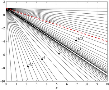
M11 noticed that for finite amplitude sub-critical slopes, (2.3) has a non-RDF, solution when forced by a vertically uniform horizontal flow

(5.7)\begin{align} \psi_{wedge}(cx,z) &=\ln\left( \frac{cx-z+1}{cx+z-1}\right)\nonumber\\ &=\ln(cx-z+1) -\ln(cx+z-1),\quad 0\leq z\leq 1,\ x>0, \end{align}

in the present notation, vanishing on $z=1$ as required and also conserving volume flux in the externally imposed oscillating flow $U.$ $\psi _{wedge}$ must be a constant, along a slope, such that

(5.8)\begin{equation} \frac{cx-z+1}{cx+z-1}=\beta, \end{equation}

where $\beta$ is a constant or

(5.9)\begin{equation} z=\gamma cx+1,\quad \gamma=\left( \frac{1-\beta}{1+\beta}\right)\langle c,x \rangle 0, \end{equation}

with a zero-depth corner at $x=0,\ z=1$ (figure 5) where the equations fail.

Figure 5.

Value of $\psi _{wedge}$ from (5.7) and a constant slope $\gamma =0.4$ (dashed red line). Contouring near the singularity at $cx=0,z=1$ and along the critical slope $z=cx$ is incomplete. Solution, also shown, would be appropriate below the critical line although not oceanographically interesting there.

This solution is valid for finite amplitude subcritical topography, under an imposed oscillating flow with magnitude increasing monotonically as the zero-depth corner is approached from $x<0.$ No radiating linear waves are generated, albeit if the slope region is finite – as is physically necessary – then the transitions to a flat bottom in both deep water and prior to the corner would have $\partial h_{1}/\partial (cx)$ discontinuous. A radiated far field, with Fourier transform again falling as $k^{-2},$ will be generated there. Solutions (5.7) might have some applicability over the large-scale sloping abyssal plains.

A topographic perturbation to a uniform slope can be dealt with in a form analogous to that done for perturbations to a flat bottom (cf. the treatment in M11 via coordinate transformation). Let $h=h_{0} +h_{1},$ where $h_{0}=\gamma cx+1$ and $h_{1}$ is a perturbation. Let $\boldsymbol {u=}( u,w) =\boldsymbol {u}_{0}+\boldsymbol {u}_{1}$, where $\boldsymbol {u}_{0}$ corresponds to the undisturbed streamfunction (5.7). Then to lowest order the boundary condition becomes

(5.10)\begin{equation} \boldsymbol{u}\boldsymbol{\cdot}\boldsymbol{\nabla}{ (h-z)}\vert _{z=\gamma x+1} \boldsymbol{\approx } \boldsymbol{u}_{0}\vert _{z=\gamma x+1}\boldsymbol{\cdot}\boldsymbol{\nabla} h_{1}+ \boldsymbol{u}_{1}\vert _{z=\gamma x+1}\boldsymbol{\cdot}\boldsymbol{\nabla} (h_{0}-z)=0. \end{equation}

Letting $\boldsymbol {u}_{1}=( \partial \psi _{1}/\partial z,-\partial \psi _{1}/\partial x) ,$ $\psi _{1}$ must satisfy the same governing hyperbolic equation as $\psi.$ With $\boldsymbol {\nabla } (h_{0}-z)=( \gamma,-1) ,$ hence with $f_1$ as in (3.2), the boundary condition is

(5.11)\begin{equation} ( 1-\gamma) f_{1}^{\prime}( ( 1-\gamma) cx) {-} ( 1+\gamma) f_{1}^{\prime}( ( 1+\gamma) cx) ={-}\boldsymbol{u}_{0}\vert _{z=\gamma x+1}\boldsymbol{\cdot}\boldsymbol{\nabla} h_{1}=Q^{\prime}(cx). \end{equation}

In the limit $\gamma \rightarrow 0,$ the slope coincides with the upper boundary.

The natural integral transform for wedge geometries is the Mellin transform (Sneddon Reference Sneddon1972) and thus defining

(5.12)\begin{equation} f_{1}^{\prime({Mln})}( s) =\mathcal{M}( f_{1}' )(s) = \int_{0}^{\infty}q^{s-1}f_{1}'( q) \, {\rm d}q,\end{equation}

with inverse transform

(5.13)\begin{equation} f_{1}'(cx) =\frac{1}{2{\rm \pi} i}\int_{\beta-i\infty }^{\beta+ i\infty}f_{1}^{{\prime}({Mln})}( s) (cx)^{{-}s}\, {\rm d}s ,\end{equation}

for some constant $\beta,$ and with corollary

(5.14)\begin{equation} \mathcal{M}( f_{1}')( \alpha x) ) =\alpha^{{-}s}f_{1}^{{\prime}({Mln})}( s) . \end{equation}

Applying $\mathcal {M}(.)$ to (5.11)

(5.15)\begin{equation} \left.\begin{array}{c@{}} \dfrac{1}{( 1-\gamma) ^{s-1}}f_{1}^{{\prime}({Mln})}( s) {-} \dfrac{1}{( 1+\gamma) ^{s-1}}f_{1}^{{\prime}({Mln})}( s) =\mathcal{M}( Q^{\prime}(cx) )\\ f_{1}^{{\prime}(\text{Mln})}( s) =\dfrac{( 1-\gamma) ^{s-1} ( 1+\gamma) ^{s-1}}{( 1+\gamma) ^{s-1}{-}( 1-\gamma) ^{s-1}} \mathcal{M}( Q^{\prime}(cx)) \end{array}\right\}, \end{equation}

for any Mellin transformable $Q^{\prime }(cx).$ The logarithmic singularity implicit here means that there is no equivalent of the Schwartz function solutions. These topographies are not pursued further here. The free propagating modes in this finite slope configuration (Wunsch Reference Wunsch1969) can be added with arbitrary amplitudes.

6. Summary

The determination of subcritical topography without ‘tidal conversion’, discussed by Maas (Reference Maas2011), can be found from a formulation in the linearized case not involving conformal-mapping analogues. As with his solutions, choice of a rapidly decaying streamfunction leads readily to a determination of a corresponding bottom topography, $h_{1}(cx)$ in an inverse problem. All solutions over the topography can be intense, with quantitative implications for ocean mixing, whether the topography is a radiating one or not. Direct solution of a governing functional equation (Manton & Mysak Reference Manton and Mysak1971) permits generation of an infinite number of non-radiating topographies for a tidal disturbance at a fixed frequency. The wider class of Schwartz function topographies are poor radiators of high-wavenumber fields.

Constraints on non-radiating topography are so great, however, that their appearance outside the laboratory or the computer seems very unlikely. One useful interpretation is that a solution at one non-radiating tidal frequency $\omega$ will, if the forcing is changed to another tidal frequency, generally produce radiation. Thus, in moving from the period of the principal lunar tide, $M_2$ at $12.42$ h to that of the principal solar tide, $S_2$ at $12.0$ hours (e.g. Zhao Reference Zhao2017), the $M_2$ null space will vanish.

The inverse problem of determining $h_{1}(cx)$ from far-field measurements will be non-unique up to topographic structures that are non-radiating (or below noise levels); see the Appendix. Primary concern will be less the inability to determine those structures, and more the necessity of observations to estimate mixing confined closely to the topography itself. The class of non-converting topographies appears to be extremely fragile and unlikely to be found in oceanographic practice.

Practical utility aside, numerous interesting theoretical extensions of this problem remain: general finite amplitude topography, super-critical reflective slopes and corners, three dimensions with rotation, non-constant $N( z)$, nonlinear interactions, shear flows, diffusion, dissipation, transient establishment and stochastic forms of topography and values of $U,$ all remain to be explored.