



1. Introduction
The Rayleigh–Taylor instability (RTI) (Rayleigh Reference Rayleigh1900; Taylor Reference Taylor1950) is a fundamental hydrodynamic instability that occurs at the interface between heavy and light fluids when the heavy fluid is supported by the light fluid against gravity. The RTI plays an important role in a number of astrophysical processes, such as supernova explosions (Burrows Reference Burrows2000; Gamezo et al. Reference Gamezo, Khokhlov, Oran, Chtchelkanova and Rosenberg2003), and is considered as a critical risk in inertial confinement fusion (ICF) implosions (Lindl Reference Lindl1998; Atzeni & Meyer-ter-vehn Reference Atzeni and Meyer-ter-vehn2004). In a typical ICF experiment, a cold spherical deuterium and tritium (DT) target coated by an ablator is irradiated either by direct laser light in the direct-drive approach (Craxton et al. Reference Craxton2015), or by X-rays emitted by a high-Z hohlraum (Lindl Reference Lindl1998) in the indirect-drive approach (Lindl Reference Lindl1995; Lindl et al. Reference Lindl, Amendt, Berger, Glendinning, Glenzer, Haan, Kauffman, Landen and Suter2004), as illustrated in figures 1(a) and 1(b), respectively. As the laser or X-ray energy is absorbed by the ablator on the outer surface of the target, the material on the ablator gets rapidly heated up and ablated off the target shell to form a hot plasma. The intense mass ablation off the target shell leads to the shell's inward acceleration and compression due to momentum conservation. As the target is compressed, its internal pressure gradually increases and causes the implosion to enter a deceleration phase; meanwhile, the kinetic energy of the shell is converted into the internal energy of DT fuels, and eventually forms a ‘hot spot’ in the centre of the target where fusion reaction occurs. As the heavy target shell is accelerated by the light ablated plasma, the interface perturbed by initial surface roughness or irradiation non-uniformity is unstable to RTI, which develops into an interchange of heavy and light fluids. The light fluid rises up, forming ‘bubbles’, while the heavy fluid falls down, forming ‘spikes’. The RTI dramatically degrades the implosion performances by compromising the shell integrity and mixing the inside DT fuel with the outside high-Z ablator. As the milestone on ignition has been achieved recently (Abu-Shawareb et al. Reference Abu-Shawareb2022; Zylstra et al. Reference Zylstra2022) at the National Ignition Facility (NIF), further improved implosion performance and higher gain are being pursued in future ICF designs where controlling the hydrodynamic instabilities remains a key factor to be considered.
Schematic of ICF target implosion: (a) direct drive, (b) indirect drive.

According to the classical linear (i.e. without mass ablation) theory (Taylor Reference Taylor1950), the interface between a heavy fluid of constant density  $\rho _h$ and a lighter fluid of constant density
 $\rho _l$ is unstable to RTI when gravity
 $\boldsymbol {g}$ points towards the lighter fluid. An infinitesimal sinusoidal perturbation on the interface would grow exponentially in time
 $\sim {\rm e}^{\gamma _{cl}t}$, at a linear growth rate
 $\gamma _{cl}=\sqrt {A_Tkg}$, where
 $k\equiv 2{\rm \pi} /\lambda$ is the perturbation wavenumber,
 $\lambda$ is the perturbation wavelength, and
 $A_T\equiv (\rho _h-\rho _l)/(\rho _h-\rho _l)$ is the Atwood number. As the amplitude of the perturbation exceeds a critical value
 $\sim 0.1\lambda$ (Ikegawa & Nishihara Reference Ikegawa and Nishihara2002), the amplitude stops growing exponentially, and the bubble of lighter fluid rises at a constant velocity inside the heavy fluid driven by the buoyancy force against the flow drag. The first nonlinear model of single-mode RTI introduced by Layzer (Reference Layzer1955) based on a potential-flow assumption with
 $A_T\approx 1$ describes the RTI growth from the early linear stage to the nonlinear bubble rising at a constant velocity. Goncharov (Reference Goncharov2002) extended Layzer's model to include finite density of the light fluid (
 $A_T \leq 1$), and found an exact solution of the equation describing the fluid motion near the bubble vertex. The asymptotic or terminal bubble velocity
 $U_b^{cl}$ depends on the dimensionality of the initial perturbation. The terminal bubble velocities for two-dimensional (2-D) and three-dimensional (3-D) initial perturbations are
 $U_b^{cl2D}=\sqrt {g(1-r_d)/3k}$ and
 $U_b^{cl3D}=\sqrt {g(1-r_d)/k}$, respectively, where
 $r_d=\rho _l/\rho _h$. In the turbulent stage of the single mode RTI, chaotic development is observed at high Reynolds numbers, where the instability undergoes seemingly random acceleration and deceleration due to complex vertex motions (Wei & Livescu Reference Wei and Livescu2012). Despite this chaotic behaviour, the mean acceleration of the bubble front eventually stabilizes at late times. Bian et al. (Reference Bian, Aluie, Zhao, Zhang and Livescu2020) found that this acceleration progress is influenced by vorticity dynamics.
Flows of plasmas typically involve rich electromagnetic processes, and the magnetic field is well known to be able to affect hydrodynamics through applying the magnetic forces directly on the macroscopic plasma flow (Chandrasekhar Reference Chandrasekhar1961) and/or through applying the anisotropic Lorentz forces microscopically on electrons to alter the electron thermal conduction, which in return influences the macroscopic plasma flow (Braginskii Reference Braginskii1965). The macroscopic magnetic forces include the magnetic pressure and the magnetic tension, both of which are typically proportional to  $B^2$ – the significance of magnetic forces in the system is usually assessed by
 $\beta \equiv {8{\rm \pi} p}/{B^2}$, where
 $p$ is the plasma thermal pressure, and
 $B$ is the magnetic field strength in Gaussian units. In the regime
 ${\beta \gg 1}$, the hydrodynamic forces dominate the plasma flow and the magnetic forces are generally neglected (Manuel et al. Reference Manuel2015; Moody et al. Reference Moody2022a; Sadler et al. Reference Sadler, Walsh, Zhou and Li2022). In the small-
 $\beta$ regime, the magnetic forces are important, and the system is governed by magnetohydrodynamics (MHD). The significance of the anisotropic heat conduction due to magnetic fields are usually assessed by the Hall parameter
 $\chi \equiv \omega _{ce}\tau _{ei}$ (Braginskii Reference Braginskii1965), where
 $\omega _{ce}$ is the electron cyclotron frequency, and
 $\tau _{ei}$ is the characteristic time of electron-ion collisions. A detailed form of the formula calculating
 $\chi$ is described in § A.1. In the regime
 $\chi \ll 1$, collisions prevent electron heat transport anisotropy (Manuel et al. Reference Manuel2015). As
 $\chi$ is of the order of 1 or even larger, electron heat transport across the magnetic field is reduced significantly (Braginskii Reference Braginskii1965; Epperlein & Haines Reference Epperlein and Haines1986). The modifications of the magnetic field on the electron thermal conduction are discussed in more detail in § 2.
The evolution of RTI affected by the magnetic forces has been studied extensively. The classical linear theory by Chandrasekhar (Reference Chandrasekhar1961) showed that a magnetic field tangential to the fluid interface can decrease the linear growth of RTI due to the magnetic tension. A critical wavelength below which RTI is suppressed is placed by the magnetic field. In another regime where the magnetic field is perpendicular to the interface, the linear growth was reported to be also decreased by the magnetic tension; however, there is no critical wavelength (Chandrasekhar Reference Chandrasekhar1961; Jun, Norman & Stone Reference Jun, Norman and Stone1995). For the nonlinear stage of RTI, Stone & Gardiner (Reference Stone and Gardiner2007a,Reference Stone and Gardinerb) performed 3-D simulations and found that strong magnetic fields can reduce mixing between the heavy and light fluids by inhibiting secondary shear instabilities, and increase the rate of growth of bubbles and spikes. Carlyle & Hillier (Reference Carlyle and Hillier2017) found that an intense tangential magnetic field slows down the growth of the rising bubbles but speeds up the falling spikes, introducing an asymmetry to the system in their 3-D simulations. Grea & Briard (Reference Grea and Briard2023) extended the potential model of Goncharov (Reference Goncharov2002) to the regime with uniform magnetic fields at various inclinations. Briard, Gréa & Nguyen (Reference Briard, Gréa and Nguyen2022) proposed a theoretical prediction for the growth of the RTI mixing zone in the presence of a vertical magnetic field based on turbulence quantities, which was verified by direct numerical simulations. Recent simulations by Briard, Gréa & Nguyen (Reference Briard, Gréa and Nguyen2024) found that the perpendicular magnetic field delays the transition to turbulence by inhibiting small-scale shear instabilities, leading to vertical stretching and rapid mixing zone growth, followed by increased turbulent dissipation that ultimately slows down the mixing zone's growth.
Other than the remarkable applications of magnetic fields in astrophysical fluid mechanics, the applications of magnetic fields in ICF have also been attracting intensive research interest as a candidate for improving ICF implosion performance. The ICF fluids are usually in a specific high-energy-density regime where the plasma thermal energy far exceeds the magnetic pressure (i.e.  $\beta \gg 1$), thus the magnetic pressure and tension applied on the fluid motion are generally considered unimportant and usually neglected in ICF-relevant simulations (Manuel et al. Reference Manuel2012b; Gao et al. Reference Gao2013; Davies et al. Reference Davies2018). However, in this regime, the Hall parameter
 $\chi$ can be significant, thus the heat flows can be notably magnetized. An externally applied magnetic field has been proposed as a promising approach to improve ICF implosion performance by reducing the electron thermal conduction and magnetically confining the DT-
 $\alpha$ burning plasma in the hot spot (Wurden et al. Reference Wurden2016; Perkins et al. Reference Perkins, Ho, Logan, Zimmerman, Rhodes, Strozzi, Blackfield and Hawkins2017). Enhanced fusion yield and temperature have been reported in cylindrical magnetized linear inertial fusion implosions (Slutz & Vesey Reference Slutz and Vesey2012; Gomez et al. Reference Gomez2014) and magnetized direct-drive ICF implosions (Chang et al. Reference Chang, Fiksel, Hohenberger, Knauer, Betti, Marshall, Meyerhofer, Séguin and Petrasso2011). Recent experiments at the NIF have also demonstrated performance enhancement from an applied magnetic field in room-temperature (‘warm’) indirect-drive implosions (Moody et al. Reference Moody2022b; Sio et al. Reference Sio2023). The effects of externally applied magnetic fields on RTI in ICF-relevant conditions were also studied via numerical simulations (Walsh et al. Reference Walsh, Chittenden, McGlinchey, Niasse and Appelbe2017; Walsh Reference Walsh2022) and experiments (Matsuo et al. Reference Matsuo, Sano, Nagatomo, Somekawa, Law, Morita, Arikawa and Fujioka2021). Walsh (Reference Walsh2022) investigated the effects of externally applied external magnetic fields in different directions on the growth of the magnetized ablative Rayleigh–Taylor instability (ARTI), considering both the magnetic tension and the magnetized heat flow, via 3-D extended-MHD simulations. The experimental work by Matsuo et al. (Reference Matsuo, Sano, Nagatomo, Somekawa, Law, Morita, Arikawa and Fujioka2021) found that the external magnetic field reduces the electron thermal conduction across the magnetic field lines, and enhances the ARTI growth.
Another type of magnetic field is self-generated by the plasmas and accompanies the evolution of hydrodynamic instabilities. It was first predicted by the theoretical works that magnetic field can be generated in RTI in laser-produced plasmas (Stamper et al. Reference Stamper, Papadopoulos, Sudan, Dean, McLean and Dawson1971; Mima, Tajima & Leboeuf Reference Mima, Tajima and Leboeuf1978; Haines Reference Haines1985; Stamper Reference Stamper1991). The Biermann battery effect was identified as the key source generating a magnetic field in RTI (Mima et al. Reference Mima, Tajima and Leboeuf1978). The misaligned temperature and density gradients generate magnetic fields via the non-zero  $\boldsymbol {\nabla } T_e \times \boldsymbol {\nabla } n_e$, where
 $T_e$ and
 $n_e$ are the electron temperature and electron number density, respectively. The laboratory astrophysical experiments by Gregori et al. (Reference Gregori2012) verified the Biermann battery mechanism at shocks associated with the collapse of protogalactic structures and its relation to protogalactic magnetic field generation. Tzeferacos et al. (Reference Tzeferacos2018) demonstrated experimentally the turbulent dynamo mechanism that turbulence is capable of, rapidly amplifying seed magnetic fields generated via Biermann battery. In experiments, simultaneous Faraday rotation was utilized to diagnose the spontaneous magnetic field in laser-produced plasmas (Stamper & Ripin Reference Stamper and Ripin1975; Raven, Willi & Rumsby Reference Raven, Willi and Rumsby1978; Stamper, McLean & Ripin Reference Stamper, McLean and Ripin1978), but such diagnostic techniques used external optical probing, thus were inadequate to measure inside the heavy plasmas opaque to the probing lights (Wagner et al. Reference Wagner2004). Proton radiography was used widely to diagnose the laser-driven magnetic field structures under more extreme plasma parameters (Li et al. Reference Li2007, Reference Li2009; Gao et al. Reference Gao, Nilson, Igumenschev, Hu, Davies, Stoeckl, Haines, Froula, Betti and Meyerhofer2012, Reference Gao2013, Reference Gao, Nilson, Igumenshchev, Haines, Froula, Betti and Meyerhofer2015; Manuel et al. Reference Manuel2012a, Reference Manuel2015). The proton radiography experiments have shown that megagauss-level magnetic fields can be generated in RTI in laser-produced plasmas (Manuel et al. Reference Manuel2012a, Reference Manuel2015; Gao et al. Reference Gao2013).
Self-generated magnetic fields not only facilitate diagnostics on the deliberate fluid structures of RTI inside hot plasmas for applications in proton radiography, but may also influence hydrodynamic evolution if intense enough. While a megagauss-level magnetic field is not strong enough to directly affect the implosion hydrodynamics in the large- $\beta$ regime, it may be strong enough to magnetize the plasma and alter the electron thermal conduction when the cyclotron frequency of the electron reaches the same order of magnitude as the electron collision frequency. The self-generated magnetic fields due to RTI in ICF is largely determined by the mass ablation feature, which brings rich physics to not only the hydrodynamics but also the generation and transportation of the magnetic fields.
When the intense laser energy is deposited on an ICF target shell, an ablated plasma outflow develops rapidly from the surface of the shell (ablation front) and creates a hot and light fluid relative to the unablated materials, as shown in figure 2. The laser-driven RTI is characterized by this ablation process on the outer surface of the shell during the acceleration phase of the implosion, and the ablative RTI (ARTI) consequently behaves quite differently from the classical RTI (CRTI) due to the mass ablation near the ablation front. It has been well known that mass ablation can mitigate the linear growth and place a linear cutoff wavenumber  $k_{c}$ in the unstable spectrum such that all modes with the perturbation wavenumber
 $k \geq k_{c}$ are linearly stable (Sanz Reference Sanz1994; Betti et al. Reference Betti, Goncharov, McCrory and Verdon1995). The penetration velocity of the ablation front into the heavy shell material – often referred to as the ablation velocity (
 $V_a$) – is a key parameter mitigating the linear growth rate (
 $\gamma _{abl}$) of ARTI, and
 $\gamma _{abl}$ can be well approximated using the Bodner–Takabe formula (Bodner Reference Bodner1974; Takabe et al. Reference Takabe, Mima, Montierth and Morse1985) obtained by fitting numerical results:
 \begin{equation} \gamma_{abl} = \tilde{\alpha} \sqrt{kg}-\tilde{\beta} k V_a, \end{equation}
where the first term on the right-hand side is the classical part, and the second term is due to mass ablation. Different values of  $\tilde {\alpha }$ and
 $\tilde {\beta }$ have to be chosen for different ablator materials, e.g.
 $\tilde {\alpha } \approx 0.94$ and
 $\tilde {\beta } \approx 2.7$ for DT ablators (Betti et al. Reference Betti, Goncharov, McCrory and Verdon1998). The growth rate curve calculated by (1.1) based on the typical initial profiles shown in figure 2(c) is plotted in figure 3 and compared with its classical counterpart, showing the linear cutoff wavelength
 $\lambda _c\approx 5\ \mathrm {\mu } \mathrm {m}$ for this set of parameters. The analytical stability theories for ARTI were then carried out in the limit of subsonic ablation flows by using complicated asymptotic matching techniques (Sanz Reference Sanz1994; Betti et al. Reference Betti, Goncharov, McCrory and Verdon1995, Reference Betti, Goncharov, McCrory, Sorotokin and Verdon1996; Goncharov et al. Reference Goncharov, Betti, McCrory, Sorotokin and Verdon1996a,Reference Goncharov, Betti, McCrory and Verdonb; Piriz, Sanz & Ibañez Reference Piriz, Sanz and Ibañez1997). The subsonic ablation – i.e. the Mach number (
 ${Ma}$) on the ablation front less than 1 – can be characterized by two dimensionless parameters (Betti et al. Reference Betti, Goncharov, McCrory and Verdon1995) that affect the density and temperature profiles near the ablation front: the Froude number
 ${Fr} \equiv V_a^2/(gL_0)$, and the power index for thermal conduction
 $\nu$ (with
 $\kappa \sim T^\nu$), where
 $L_0$ is the characteristic thickness of the ablation front, which is proportional to the minimal density gradient scale length
 $L_m$ as
 $L_0 \equiv L_m \nu ^{\nu }/(\nu +1) ^{\nu +1}$. In ARTI, where the fluid density has non-uniform spacial profiles as plotted in figure 2(c), the Atwood number is typically defined as
 $A_T\equiv (\rho _a-\rho _{bo})/(\rho _a+\rho _{bo})$, where
 $\rho _a$ is the density on the ablation front,
 $\rho _{bo} = \rho _a \mu (kL_0)^{\nu }$ is the density of the blowoff material,
 $\mu =(2/\nu )^{1/\nu }/\varGamma (1+1/\nu )+0.12/\nu ^2$, and
 $\varGamma (x)$ is the gamma function, as presented by the comprehensive theory of Goncharov et al. (Reference Goncharov, Betti, McCrory, Sorotokin and Verdon1996a,Reference Goncharov, Betti, McCrory and Verdonb).
The simulation set-up. (a) A schematic of the acceleration stage of a direct-drive target. The area in the red box near the target surface is the domain of the simulation. (b) The contour of the initial density. (c) The initial profile for  $\rho$ (blue solid line),
 $T$ (red dashed line) and
 $v_z$ (green dash-dotted line) along the
 $z$ axis.


While ablation is stabilizing the linear growth of ARTI, it has been known that ablation destabilizes ARTI in the nonlinear stage through the vortex acceleration mechanism in both 2-D (Betti & Sanz Reference Betti and Sanz2006) and 3-D (Yan et al. Reference Yan, Betti, Sanz, Aluie, Liu and Frank2016) geometry. The vortices generated near spike tips are transported into the bubble and provide centrifugal forces to the bubble vertex, thereby accelerating the nonlinear terminal bubble velocity above the classical values predicted by Goncharov (Reference Goncharov2002). The vortex acceleration mechanism was found to be especially significant for the small-scale 3-D bubbles (Yan et al. Reference Yan, Betti, Sanz, Aluie, Liu and Frank2016) in ARTI. In contrast to CRTI, which transits to a turbulent state later on, it was found in simulations that the spikes are significantly suppressed, and the late-time nonlinear stage ARTI is far from a turbulent state due to mass ablation (Zhang et al. Reference Zhang, Betti, Yan, Zhao, Shvarts and Aluie2018).
The large temperature gradient created by the ablation provides the well-known Nernst effect (Nishiguchi et al. Reference Nishiguchi, Yabe, Haines, Psimopoulos and Takewaki1984) on the magnetic fields. The Nernst effect is known to provide an additional convective velocity against the direction of temperature gradient on the magnetic field, which will significantly affect the transport process of the magnetic field. One-dimensional (1-D) simulations showed that the Nernst effect convects the magnetic field towards the high-density region in laser-driven ablation plasma, and the magnetic field is significantly compressed and amplified (Nishiguchi et al. Reference Nishiguchi, Yabe, Haines, Psimopoulos and Takewaki1984; Nishiguchi, Yabe & Haines Reference Nishiguchi, Yabe and Haines1985).
The pioneering simulations (Srinivasan, Dimonte & Tang Reference Srinivasan, Dimonte and Tang2012; Srinivasan & Tang Reference Srinivasan and Tang2012, Reference Srinivasan and Tang2013) were performed on the magnetic field generation and evolution for 2-D single-mode and multi-mode RTI in a stratified two-fluid plasma using a Hall MHD model. However, neither the mass ablation due to heat conduction nor the Nernst effect was considered in those simulations. Our previous simulations (Zhang et al. Reference Zhang, Li, Xin, Yan, Wan, Zhang and Zheng2022) including the heat conduction and the Nernst effect showed that  $\sim$100 T magnetic fields – a challenging value to be obtained directly in the laboratory using superconductor coils (Shneerson, Dolotenko & Krivosheev Reference Shneerson, Dolotenko and Krivosheev2014) – can be generated via ARTI, and the Nernst effect is a critical factor determining the magnetic fields’ peak amplitude and spacial distribution. As feedback to hydrodynamics, the self-generated magnetic field changes electron thermal conduction by magnetizing the plasma. Analytical study of the effects of self-generated magnetic fields on ARTI in the linear regime (García-Rubio et al. Reference García-Rubio, Betti, Sanz and Aluie2021) showed that the magnetic field affects the ARTI growth by bending the heat flux lines, and it destabilizes ARTI for moderate Froude numbers
 ${Fr}$ and stabilizes ARTI for large
 ${Fr}$, which is consistent with our 2-D simulations (Zhang et al. Reference Zhang, Li, Xin, Yan, Wan, Zhang and Zheng2022). The 2-D simulations also showed that both the linear growth rate and the nonlinear amplitude of ARTI are increased by approximately
 $10\,\%$ due to the magnetic feedback (Cui et al. Reference Cui, Yang, Ma, Zhang, Xu, Chen, Li, Shao and Zhang2024). The simulations on the stagnation phase of an ICF implosion showed that the magnetic field can cool the spikes and weaken the ablative stabilization, which harmfully increases the heat loss of the hot spot (Walsh et al. Reference Walsh, Chittenden, McGlinchey, Niasse and Appelbe2017).
In this work, we present the simulation results for the evolution of the magnetic field generated via 3-D ICF-relevant single-mode ARTI in a quasi-equilibrium frame of the acceleration phase of implosion. Important physics – including ablation, Nernst effect, resistance and magnetized heat conduction – is taken into account to sketch more realistic magnetic fields’ generation, evolution and feedback to ARTI evolution. It is found that  ${\sim } 10^3$ T magnetic fields can be generated via 3-D ARTI, which is an order of magnitude stronger than that found in our previous 2-D work (Zhang et al. Reference Zhang, Li, Xin, Yan, Wan, Zhang and Zheng2022). Such strong magnetic fields are able to profoundly alter local hydrodynamics by modifying the electron thermal conduction, and speed up the growth of the spikes.
The rest of the paper is organized as follows. In § 2, the physical model and the numerical method are outlined. In § 3, the simulation settings are presented. In § 4.1, the simulation results on the magnetic fields’ generation and transportation are presented and analysed. In § 4.2, the feedback of a self-generated magnetic field on 3-D ARTI nonlinear evolution is investigated. Section 5 is a summary. In Appendix A, the magnetized plasma transport coefficients used in this paper are presented.
2. Physics models
The simulations on 3-D ARTI and self-generated magnetic fields are carried out in planar geometry using the hydrodynamic code ART. Specifically designed for modelling ARTI in ICF-relevant scenarios, ART has been used in a number of recent works (Betti & Sanz Reference Betti and Sanz2006; Yan et al. Reference Yan, Betti, Sanz, Aluie, Liu and Frank2016; Zhang et al. Reference Zhang, Betti, Yan, Zhao, Shvarts and Aluie2018, Reference Zhang, Betti, Yan and Aluie2020, Reference Zhang, Li, Xin, Yan, Wan, Zhang and Zheng2022; Xin et al. Reference Xin, Yan, Wan, Sun, Zheng, Zhang, Aluie and Betti2019, Reference Xin, Liu, Jiang, Yan, Li, Wan, Sun and Zheng2023; Li et al. Reference Li, Yan, Zhao, Zheng, Zhang and Lu2022, Reference Li, Yan, Zhao, Zheng, Zhang and Lu2023, Reference Li, Yan, Zhao, Wu, Wang and Zou2024; Fu et al. Reference Fu, Zhang, Cai and Zhu2023b; Liu et al. Reference Liu, Zhang, Xin, Pu, Li, Tao, Sun, Yan and Zheng2023). Code ART solves the single-fluid equations in 2-D/3-D Cartesian coordinates, and this paper focus on the 3-D geometry. The hydrodynamic equations are
 $$\begin{gather} \frac{\partial \rho}{\partial t} +\boldsymbol{\nabla} \boldsymbol{\cdot} (\rho \boldsymbol{v})=0, \end{gather}$$
 $$\begin{gather}\frac{\partial\rho \boldsymbol{v}}{\partial t}+\boldsymbol{\nabla} \boldsymbol{\cdot} (\rho \boldsymbol{vv} )={-}\boldsymbol{\nabla} p +\rho\boldsymbol{g}, \end{gather}$$
 $$\begin{gather}\frac{\partial \epsilon}{\partial t}+\boldsymbol{\nabla}\boldsymbol{\cdot} [(\epsilon+p)\boldsymbol{v}] =\rho\boldsymbol{v}\boldsymbol{\cdot}\boldsymbol{g}-\boldsymbol{\nabla}\boldsymbol{\cdot} \boldsymbol{q}, \end{gather}$$
where  $\rho$ is the mass density,
 $\boldsymbol {v}$ is the macroscopic single-fluid velocity of the plasma,
 $p$ is the plasma thermal pressure, and
 $\boldsymbol {g}$ is the acceleration. The equation of state of an ideal gas is used, the plasma energy is
 $\epsilon =[{p}/{(\gamma -1)}]+[{\rho v^2}/{2}]$, and
 $\gamma ={5}/{3}$ is the specific heat ratio. As discussed in § 1, the magnetic forces have been neglected in (2.2). The low viscosity in high-energy-density plasma flows commonly neglected in the simulations on hydrodynamic instabilities (Betti & Sanz Reference Betti and Sanz2006; Wang et al. Reference Wang, Ye, Sheng, Don, Li and He2010; Zhang et al. Reference Zhang, Betti, Yan, Zhao, Shvarts and Aluie2018; Li et al. Reference Li, Yan, Zhao, Zheng, Zhang and Lu2022) is not considered in this work either. Although ARTI is in a regime with high Reynolds numbers (
 $Re \sim 10^5$ evaluated using the viscosity coefficient in Huba Reference Huba1998), the ablative effect in ARTI flattens the fine structures typically generated in CRTI, and prevents the transition to a turbulent state (Zhang et al. Reference Zhang, Betti, Yan, Zhao, Shvarts and Aluie2018).
The heat flux  $\boldsymbol {q}$ contributes to the energy equation (2.3) via a thermal conduction term
 $-\boldsymbol {\nabla } \boldsymbol {\cdot } \boldsymbol {q}$, which is treated separately in a Strang-splitting way (Strang Reference Strang1968) by solving the heat conduction equation
 \begin{equation} \rho c_v\,\frac{\partial T}{\partial t}={-}\boldsymbol{\nabla}\boldsymbol{\cdot} \boldsymbol{q}, \end{equation}
after solving the pure hydrodynamic equations (2.1)–(2.3) without the  $-\boldsymbol {\nabla } \boldsymbol {\cdot } \boldsymbol {q}$ term. Here,
 $T$ is the kinetic temperature including the Boltzmann constant, and
 $c_v$ is the constant-volume specific heat capacity. An MUSCL-Hancock scheme (van Leer Reference van Leer1984) with an HLLC (Harten, Lax & van Leer Reference Harten, Lax and van Leer1983) approximate Riemann solver is used as the hydrodynamic solver with second-order accuracy in both space and time to solve the hydrodynamics equations. For each computational time step, the pure hydrodynamic equations (2.1)–(2.3) without the
 $-\boldsymbol {\nabla } \boldsymbol {\cdot } \boldsymbol {q}$ term are advanced first, followed by an intermediate update of
 $T$ and
 $p$ with the help of the equation of state. Equation (2.4) is then solved to update
 $T$ once again, using a temporally implicit scheme to avoid the strict time step (
 $\Delta t$) requirement of explicit diffusion equation solvers. Then
 $p$ and
 $\epsilon$ are updated with the newly calculated
 $T$ using the equation of state before entering the next time step. The single-temperature approximation of the plasma is applied so that the electron temperature
 $T_e$ and ion temperature
 $T_i$ are equal (i.e.
 $T_e=T_i=T$), since the relaxation time (
 ${\sim }10^{-4}$ ns evaluated using the formula in Huba Reference Huba1998) for electron–ion temperature equilibration on the ablation front is much shorter than the time scale of the ARTI evolution. For the magnetic-free cases, the classical Spitzer–Harm model (Spitzer & Härm Reference Spitzer and Härm1953) is used to calculate the heat flux
 $\boldsymbol {q}$ in (2.4) as
 \begin{equation} \boldsymbol{q}_{sh} ={-}\kappa_{sh}\,\boldsymbol{\nabla} T, \end{equation}
where  $\kappa _{sh}$ is the Spitzer–Harm conductivity without flux limiter. The heat flux limiters that are often used in high-energy-density fluid simulations in various regimes to cap the unphysically large heat fluxes given by (2.5) and to match experiments are not applied in the simulations in this paper, since the maximum ratio of
 $q$ to the free-stream heat flux in the simulations always reads below 0.06, a commonly used flux-limiting threshold (Bell Reference Bell1985; Craxton et al. Reference Craxton2015). Equation (2.5) also does not include the non-local electron heat transport that is attracting research interest. Our previous simulations (Li et al. Reference Li, Yan, Zhao, Zheng, Zhang and Lu2022, Reference Li, Yan, Zhao, Zheng, Zhang and Lu2023) showed that the non-local electron heat transport can mitigate ARTI growths. Recent work by Campbell et al. (Reference Campbell2022) demonstrated the need to account for suppression of Biermann battery generation due to non-local effects by comparing experimental data and simulations. However, modelling the non-local electron heat transport is computationally costly in 3-D simulations, and beyond the scope of this paper. In the simulations, we set the single fluid to be a DT plasma with the number ratio 1 : 1. The advantage of using a DT plasma in the simulations is that it can avoid complex physics such as radiation transport coming from higher-Z materials.
The equation of magnetic field ( $\boldsymbol {B}$) evolution can be derived readily from Ampère's law, Faraday's law, and the momentum equation of electrons (Nishiguchi et al. Reference Nishiguchi, Yabe, Haines, Psimopoulos and Takewaki1984), and formulated in Gaussian units as
 \begin{equation} \frac{\partial\boldsymbol{B}}{\partial t}= \underbrace{\boldsymbol{\nabla}\times(\boldsymbol{v}\times\boldsymbol{B})}_{{I}} +\underbrace{\frac{c}{e}\,\boldsymbol{\nabla}\times\left(\frac{\boldsymbol{\nabla} p_e}{n_e}\right)}_{{II}} -\underbrace{\frac{c}{4{\rm \pi} e}\,\boldsymbol{\nabla}\times\left[\frac{(\boldsymbol{\nabla}\times\boldsymbol{B})\times\boldsymbol{B}}{n_e}\right]}_{{III}} -\underbrace{\frac{c}{e}\,\boldsymbol{\nabla}\times\frac{\boldsymbol{R}}{n_e}}_{{IV}}, \end{equation}
where  $e$ is the elementary charge carried by an electron,
 $c$ is the speed of light in vacuum,
 $n_e$ is the number density of the electrons, and
 $p_e$ is the isotropic pressure of the electrons. Isotropic electron pressure has been used in (2.6), since the pressure anisotropy that is crucial in collisionless plasmas is not important in collisional plasmas (Egedal, Le & Daughton Reference Egedal, Le and Daughton2013; Tubman et al. Reference Tubman2021) as in this regime. Here,
 $\boldsymbol {R}=\boldsymbol {R}_{{u}}+\boldsymbol {R}_{{T}}$ as the transfer of momentum from ions to electrons caused by collisions consists of two parts: (i) the thermal force
 $\boldsymbol {R}_{{T}}$ due to the gradient of the electron temperatures; and (ii) the friction force
 $\boldsymbol {R}_{{u}}$ due to the relative velocity of electrons and ions. These
 $\boldsymbol {R}_{{T}}$ and
 $\boldsymbol {R}_{{u}}$ are usually formulated in a Braginskii-like form (Braginskii Reference Braginskii1965) as
 $$\begin{gather} \boldsymbol{R}_{{T}}={-}\beta_{{\parallel}}^{uT}\,\nabla_{{\parallel}}T_e -\beta_{{\perp}}^{uT}\,\nabla_{{\perp}}T_e -\beta_{\land}^{uT}\boldsymbol{b}\times\boldsymbol{\nabla} T_e, \end{gather}$$
 $$\begin{gather}\boldsymbol{R}_{{u}}={-}\alpha_{{\parallel}}\boldsymbol{u}_{{\parallel}} -\alpha_{{\perp}}\boldsymbol{u}_{{\perp}} +\alpha_{\land}\boldsymbol{b}\times \boldsymbol{u}, \end{gather}$$
where  $\boldsymbol {b} \equiv \boldsymbol {B}/|\boldsymbol {B}|$ is the unit direction vector parallel to the magnetic field, and
 $\boldsymbol {u} =\boldsymbol {u}_{{e}}-\boldsymbol {u}_{{i}}$ is the relative velocity of electrons and ions that can be associated with the magnetic field via Ampère's law
 $\boldsymbol {u}=-c\,\boldsymbol {\nabla }\times \boldsymbol {B}/(4{\rm \pi} n_ee)$. Also,
 $\nabla _{\parallel }T_e$ and
 $\nabla _{\perp }T_e$ are the components of the temperature gradient parallel and perpendicular to the direction of
 $\boldsymbol {B}$, respectively, and
 $\boldsymbol {u}_{\parallel }$ and
 $\boldsymbol {u}_{\perp }$ are the components of
 $\boldsymbol {u}$ parallel and perpendicular to the direction of
 $\boldsymbol {B}$, respectively. Here,
 $\beta _{\parallel }^{uT}$,
 $\beta _{\perp }^{uT}$,
 $\beta _{\land }^{uT}$,
 $\alpha _{\parallel }$,
 $\alpha _{\perp }$ and
 $\alpha _{\land }$ are the plasma transport coefficients that are detailed in Appendix A. The Braginskii formulation on the transport coefficients is a classical model that has been used widely in collisional astrophysical and high-energy-density plasmas (Velikovich, Giuliani & Zalesak Reference Velikovich, Giuliani and Zalesak2019; Sadler, Walsh & Li Reference Sadler, Walsh and Li2021; Tapinou et al. Reference Tapinou, Wheatley, Bond and Jahn2023; Kopp & Yanovsky Reference Kopp and Yanovsky2024), including ARTI-relevant problems (García-Rubio et al. Reference García-Rubio, Betti, Sanz and Aluie2021; Zhang et al. Reference Zhang, Li, Xin, Yan, Wan, Zhang and Zheng2022). Improved transport coefficients with less physical approximation than Braginskii's were obtained later (Epperlein & Haines Reference Epperlein and Haines1986; Ji & Held Reference Ji and Held2013; Davies et al. Reference Davies, Wen, Ji and Held2021) through fitting numerical solutions of the Fokker–Planck equation with different fitting strategies. It was reported in Davies et al. (Reference Davies, Wen, Ji and Held2021) that the fitted transport coefficients can give physically incorrect results under certain conditions. Davies et al. (Reference Davies, Wen, Ji and Held2021) clarified that the only serious error in Braginskii's coefficients is an overestimation of perpendicular resistivity (
 $\alpha _{\perp }$) at intermediate Hall parameters (
 $\chi >2$ up to
 $\sim$100), while the errors in the Epperlein and Haines coefficients are particularly severe, giving increasing
 $\beta _{\parallel }^{uT}-\beta _{\perp }^{uT}$ and
 $\alpha _{\parallel }-\alpha _{\perp }$ for
 $\chi < 1$ when they should decrease linearly to zero. In this work, we still utilize the classical Braginskii coefficients in most of the simulations, also to be consistent with our previous work on 2-D ARTI (Zhang et al. Reference Zhang, Li, Xin, Yan, Wan, Zhang and Zheng2022) for a fair comparison. Moreover, a few simulation cases (cases xiv–xvi) are performed with the Davies et al. (Reference Davies, Wen, Ji and Held2021) transport coefficients to show the difference introduced by different transport models.
Term I of (2.6) is usually known as the convection term that freezes the magnetic field along with the plasma. Term II is the baroclinic term (also known as the Biermann battery) generating the self-magnetic field through the misaligned density and pressure gradients, since  $c\,\boldsymbol {\nabla }\times (\boldsymbol {\nabla } p_e /n_e)/e=c\,\boldsymbol {\nabla } p_e \times \boldsymbol {\nabla } n_e /{(en_e^2)}$. Term III is often referred to as the Hall term, which is neglected since the ratio of III to II approximately equals
 $1/\beta \ll 1$ in the regimes covered by this work. Term IV brings the effects of collisions, including the magnetic dissipation related to
 $\boldsymbol {R}_{{u}}$ and the Nernst effect related to
 $\boldsymbol {R}_{{T}}$. Bringing in the expressions for
 $\boldsymbol {R}_{{T}}$ and
 $\boldsymbol {R}_{{u}}$, term IV of (2.6) can be written as
 \begin{align} -\frac{c}{e}\,\boldsymbol{\nabla}\times\frac{\boldsymbol{R}}{n_e} &=\frac{c}{e}\,\boldsymbol{\nabla}\times\left(\frac{\beta_{{\parallel}}^{uT}\,\boldsymbol{\nabla} T_e }{n_e}\right) -\frac{c}{e}\,\boldsymbol{\nabla}\times\left[\frac{(\beta_{{\parallel}}^{uT} -\beta_{{\perp}}^{uT})(\boldsymbol{b} \times\boldsymbol{\nabla} T_e)\times\boldsymbol{B}}{B n_e}\right]\nonumber\\ &\quad -\frac{c}{e}\,\boldsymbol{\nabla}\times\left(\frac{\beta_{\land}^{uT}\,\boldsymbol{\nabla} T_e\times \mathbf{B} }{ B n_e}\right)-\frac{c^2}{4{\rm \pi} e^2}\,\boldsymbol{\nabla}\nonumber\\ &\quad \times\left\{\frac{\alpha_{{\parallel}}\,\boldsymbol{\nabla}\times\boldsymbol{B}-\alpha_{\land}\boldsymbol{b} \times(\boldsymbol{\nabla}\times\boldsymbol{B})-(\alpha_{{\perp}}-\alpha_{{\parallel}})\boldsymbol{b} \times[\boldsymbol{b}\times(\boldsymbol{\nabla}\times\boldsymbol{B})]}{n_e^2}\right\}. \end{align}
The first term on the right-hand side of (2.9) has no contribution in a fully ionized plasma (Sadler et al. Reference Sadler, Walsh and Li2021), while the combination of the second and third terms can be rewritten as  $\boldsymbol {\nabla }\times [(\boldsymbol {V}_{{N}}+\boldsymbol {V}_{{CN}})\times \boldsymbol {B}]$, where
 $\boldsymbol {V}_{{N}}$ and
 $\boldsymbol {V}_{{CN}}$ are often referred as the Nernst velocity and the cross-gradient Nernst velocity in the forms
 $$\begin{gather} \boldsymbol{V}_{{N}}={-}\frac{c \beta_{\land}^{uT}}{e B n_{e}}\,\boldsymbol{\nabla} T_e, \end{gather}$$
 $$\begin{gather}\boldsymbol{V}_{{CN}}={-}\frac{c(\beta_{{\parallel}}^{uT}-\beta_{{\perp}}^{uT})( \boldsymbol{b}\times\boldsymbol{\nabla} T_e)}{e B n_e}, \end{gather}$$
respectively. Here,  $\boldsymbol {V}_{{N}}$ is along the direction opposite to
 $\boldsymbol {\nabla } T_e$ so that it convects the magnetic field in the direction of the heat flow;
 $\boldsymbol {V}_{{CN}}$ is in the direction of
 $-\boldsymbol {b}\times \boldsymbol {\nabla } T_e$, which causes the magnetic field to convect along the isothermal line. Also,
 $V_{N}$ is much larger than
 $V_{CN}$ where
 $\chi \sim {T_e^{3/2}B}/{n_e} \ll 1$, thus the contribution of
 $V_{N}$ is dominating with moderate magnetic fields. The last term on the right-hand side of (2.9) reflects the diffusion of the magnetic field in different directions. Both the Nernst effect and the magnetic field diffusion are implemented in our simulations.
The intense magnetic field changes the process of electron heat conduction by magnetizing the plasma. While the magnetic field is not expected to be strong enough to significantly affect the implosion hydrodynamics via the momentum equation in ICF-relevant plasmas, it may be strong enough to magnetize the plasma and make the heat flux  $\boldsymbol {q}$ anisotropic via the Lorentz forces applied on the electrons moving in different directions with respect to the local magnetic field. The magnetic field leads to a flux-limiting effect perpendicular to
 $\boldsymbol {B}$ compared to the classical Spitzer–Harm heat flux
 $\boldsymbol {q}_{sh}$, which was derived in a magnetic-free plasma. In addition, the magnetic field generates a heat flux component known as the Righi–Leduc heat flux perpendicular to both
 $\boldsymbol {B}$ and
 $\boldsymbol {\nabla } T$. The heat flux in a magnetized plasma to feed (2.4) reads as
 \begin{equation} \boldsymbol{q}_{mag} ={-}\kappa_{{\parallel}}\,\nabla_{{\parallel}}T_e -\kappa_{{\perp}}\,\nabla_{{\perp}}T_e -\kappa_{\land}\boldsymbol{b}\times\boldsymbol{\nabla} T_e, \end{equation}
where  $\kappa _{\parallel }$,
 $\kappa _{\perp }$ and
 $\kappa _{\land }$ are the conduction coefficients in magnetized plasma. The detailed forms of
 $\kappa _{\parallel }$,
 $\kappa _{\perp }$ and
 $\kappa _{\land }$ are given in Appendix A. Along the direction parallel to
 $\boldsymbol {B}$, the magnetic field has no modification on the electron conduction, and
 $\kappa _{\parallel }$ is identical to
 $\kappa _{sh}$. Also,
 $\kappa _{\perp }$ is smaller than
 $\kappa _{\parallel }$ where
 $B\neq 0$,
 $\kappa _{\perp }$ retreats to
 $\kappa _{sh}$ where
 $B=0$, and
 $\kappa _{\perp }$ decreases as
 $\chi$ increases, leading to a flux-limiting effect perpendicular to the magnetic fields. The term
 $-\kappa _{\land } \boldsymbol {b}\times \boldsymbol {\nabla } T_e$, known as the Righi–Leduc heat flux, makes a special contribution to the heat conduction in a magnetized plasma. Both (2.6) and (2.12) have been implemented in ART, with the option to turn on and off different terms to be able to investigate a specific physical process. In this paper,
 $\boldsymbol {q}_{mag}$ and
 $\boldsymbol {q}_{sh}$ are switched in the calculation of
 $\boldsymbol {\nabla } \boldsymbol {\cdot } \boldsymbol {q}$ in (2.4) in the simulations to compare the 3-D ARTI evolution with and without the magnetized heat fluxes and investigate the magnetic feedback on ARTI.
3. Simulation settings
In the ART simulations, ARTI is initialized to grow from small perturbations on top of a quasi-equilibrium state abstracted from a typical profile of direct-drive NIF targets as shown in figure 2. In figure 2(a), the red box outlines the region on the target surface where ARTI occurs, which has been selected as the computational domain for the simulations in this paper. A planar approximation is valid as long as the target thickness, mode wavelength and conduction zone region are much smaller than the target radius. This condition is satisfied during most of the acceleration stage. The initial hydrodynamic profiles of a DT ablator used in case i in table 1, shown in figure 2(c), are similar to those of a direct-drive ignition target (McKenty et al. Reference McKenty, Goncharov, Town, Skupsky, Betti and McCrory2001) during the acceleration phase of an implosion driven by the 1.5 MJ, 351 nm wavelength lasers.
Parameters and physical options of the simulation cases in this paper. All simulation cases are conducted with grid resolution 10 grid points per micron. The Mach numbers  $Ma$ are calculated on the bottom boundaries. If the
 $\boldsymbol {q}_{mag}$ option is off, then
 $\boldsymbol {q}_{sh}$ is used in (2.4). If the
 $\boldsymbol {q}_{mag}$ option is on, then
 $\boldsymbol {q}_{mag}$ is used in (2.4) instead.

As shown in figure 2(b), the cold and dense unablated DT shell is placed on top of the ablated DT plasma with a higher temperature but a lower density. The initial ablation front (the interface between the dense and the ablated plasma) is located at  $z_0=70\ \mathrm {\mu } {\rm m}$, with the peak density
 $\rho _a=5.3$ g cm
 $^{-3}$ reached on the ablation front. The quasi-equilibrium state is obtained by integrating the 1-D hydrodynamic equilibrium equations in the frame of reference of the shell from the ablation front towards both sides. Above the ablation front, the shell is performing like a solid piston, so
 $v_z = V_a$ is initially set in the shell. In the ablation area below the ablation front, the 1-D profiles can be found by neglecting the derivatives on
 $t$,
 $x$ and
 $y$ in (2.1)–(2.3). The ablation front is kept approximately fixed in the middle of the computational domain by balancing the ablative pressure with a dynamically adjusted effective gravity
 $\boldsymbol {g}$. This is equivalent to solving the fluid equations in the frame of reference of the accelerated shell. The initial gravity is
 ${g}(0)=100$
 $\mathrm {\mu }$m ns
 $^{-2}$. Since the shell mass decreases due to ablation, the effective acceleration
 $g(t)$ is slowly and automatically adjusted in time during the simulation to keep the ablation front approximately fixed in space, i.e.
 $g(t) = [(p + \rho u^2)_{bot}-(p + \rho u^2)_{top}]/M_{tot}$, where the subscripts ‘bot’ and ‘top’ indicate the integral values at the bottom and top boundaries, respectively, and
 $M_{tot}$ is the total mass of the remaining plasma in the computational domain. The quasi-equilibrium hydrodynamic profiles together with a time-dependent but spatially uniform gravity
 $g(t)$ are used to mimic an already well-established quasi-equilibrium ICF plasma slowly evolving under the isobaric assumption also used in the analytical ARTI theories (Goncharov et al. Reference Goncharov, Betti, McCrory, Sorotokin and Verdon1996a,Reference Goncharov, Betti, McCrory and Verdonb). The ablation velocity is
 $V_a = 3.5$
 $\mathrm {\mu }$m ns
 $^{-1}$, and the ablation pressure (i.e. the pressure at the ablation surface) is
 $p_a = 140$ Mbar. In this quasi-equilibrium state, the unablated plasma flows in from the top boundary approximately at the ablation velocity, and the ablated plasma flows out through the bottom boundary at a very high velocity, as shown in figure 2(c).
Our simulations do not include the underdense region where the lasers are interacting with the plasma, therefore we do not handle laser absorption directly. Instead, the laser energy transported towards the ablation front is simulated by a constant bottom boundary heat flux  $Q_{bottom} = 6.0\ \mathrm {MW}\ \mathrm {\mu } \mathrm {m}^{-2}$, which is calculated self-consistently with the Spitzer–Harm model on the basis of the 1-D hydrodynamic profiles. A characteristic Mach number that is also the maximum in the simulation zone is evaluated on the bottom boundary as
 ${Ma}=0.43$, indicating a subsonic outflow. The Mach number decreases rapidly from the bottom boundary towards the ablation front neighbourhood where ARTI grows (typically
 $Ma < 0.3$). The Atwood number is
 $A_T= 0.66$, and the Froude number is
 ${Fr}=4.61$. In addition to the above parameters associated with the initial hydrodynamic profiles in figure 2(c), we also use different
 $V_a$,
 $P_a$ and
 $g_0$ to explore the ARTI and magnetic evolution in a broader parameter space. The detailed simulation parameters are listed in table 1.
In order to seed 3-D ARTI, the velocity perturbations ( $\boldsymbol {v}_{{p}}$) are initialized around the ablation front in a divergence-free form as
 $$\begin{gather} v_{px}=v_{p0} \sin(k x) \exp({-}k\vert z-z_0 \vert), \end{gather}$$
 $$\begin{gather}v_{py}=v_{p0} \sin(k y)\exp({-}k\vert z-z_0 \vert), \end{gather}$$
 $$\begin{gather}v_{pz}=v_{p0} [\cos(k x)+\cos(k y)]\exp({-}k\vert z-z_0 \vert), \end{gather}$$
where  $v_{p0}$ is the magnitude of the initial velocity perturbation, set as
 $v_{p0} = 0.5$
 $\mathrm {\mu }$m ns
 $^{-1}$. A typical simulation is carried out with a simulation box 140
 $\mathrm {\mu }$m in the
 $z$ direction, while the widths in the
 $x$ and
 $y$ directions are chosen to be
 $\lambda$. A uniform Cartesian grid is used, with resolution 10 grid points per micron, and the grid independence is checked to ensure numerical convergence. Periodic boundary conditions are applied in the
 $x$ and
 $y$ directions for both the hydrodynamic quantities and the magnetic field. The inflow/outflow boundary conditions are used on the top/bottom boundaries in the
 $z$ direction for hydrodynamics to facilitate the ablated plasma flow to leave the simulation zone smoothly. The adiabatic boundary condition is applied for the top boundary, i.e.
 $\partial T/\partial z=0$. And the fixed-flux boundary condition is applied for the bottom boundary, i.e.
 $-\kappa \,\partial T/\partial z=Q_{bottom}$. The top and bottom boundary conditions for the magnetic field are set as
 $\partial (v_z \boldsymbol {B}) /\partial z = 0$.
4. Results and discussions
A series of ART simulations have been performed to study the generation, evolution and feedback of the self-generated magnetic fields accompanying ARTI in 3-D geometry. As outlined in § 2, we have set up an idealized but still experimentally relevant scenario to be able to focus on the pure ARTI evolution and the magnetic generation in the ART simulations. This approach also enables us to conveniently investigate the factors (i.e. geometric dimensions, ablation, the Nernst effects and magnetized heat fluxes) that influence RTI and/or magnetic evolution by switching these modules in the simulations on and off while still allowing the simulations to start from virtually the same quasi-equilibrium hydrodynamic state, for a relatively fair comparison. Our previous 2-D work (Zhang et al. Reference Zhang, Li, Xin, Yan, Wan, Zhang and Zheng2022) demonstrated that the effects involving the self-generated magnetic fields are more profound for short-wavelength modes with  $\lambda$ close to the linear cutoff wavelength
 $\lambda _c \equiv 2{\rm \pi} / k_c$. Therefore, the simulation cases are more focused on the short-wavelength regime in this work.
4.1. Evolution of the self-generated magnetic field
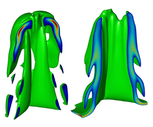
The evolution of ARTI from the linear stage up to the highly nonlinear stage in case i is illustrated in figure 4. It is shown that a clear 3-D bubble is formed in the centre of the simulation box as the perturbation amplitude increases, with the heavy fluid surrounding the bubble penetrating down into the light fluid. The ‘bubble–spike’ topology is significantly different from its 2-D counterpart. A bubble tends to expand to form a round shape, as shown in figure 4(b) at the early nonlinear stage ( $t=1.4$ ns). However, as the bubble grows larger and longer, it expands but gets confined by the four adjacent bubbles due to the geometrical characteristic of the ‘single square mode’ (Dahlburg et al. Reference Dahlburg, Gardner, Doolen and Haan1993) system that is periodic along both
 $x$ and
 $y$ directions. The squeezing between adjacent bubbles leads to square-like bubble shapes in the highly nonlinear stages, as illustrated by figures 4(c,d). Finer grids have been used to make sure that this feature is not caused by grid resolutions. The ratio of the volume of the bubble to the simulation box plotted in figure 4(e) also demonstrates the growth of the bubble.
(a–d) The ARTI bubble structures at different times, from the linear stage ( $t = 0.8$ ns) to the nonlinear stage (
 $t = 1.4$, 2.0 and 2.5 ns), in case i. (e) The ratio of the volume of the bubble to the simulation box
 $\sigma _b$ versus time in case i.

The magnetic field generation is found to be correlated with the growth of ARTI. The magnetic fields at the linear stage in cases i (without Nernst) and ii (with Nernst) are illustrated in figures 5(a) and 5(b), respectively. Note that in cases i and ii, the magnetic feedbacks are both kept off, so the hydrodynamics in these two cases are essentially identical. Figure 5(a) shows that the magnetic fields are mostly generated near the ablation front where the baroclinic source, i.e. term II of (2.6), is concentrated. The generated magnetic field then expands with the ablated material and enters the low-density area by convection. As a result, a magnetic field layer is formed below the ablation front. Case ii with the Nernst effects turned on clearly shows the influence from  $\boldsymbol {V}_{{N}}$ and
 $\boldsymbol {V}_{{CN}}$, which are largely determined by the amplitude of the magnetic field and
 $\boldsymbol {\nabla } T_e$ (see (2.10) and (2.11)). The Nernst velocity
 $\boldsymbol {V}_{{N}}$ tends to convect the magnetic field against the ablation front (figure 5b), where
 $T_e$ transits abruptly from the cold dense shell to the ablated low-density plasma, thus
 $\boldsymbol {V}_{{N}}$ is towards the shell. The cross-gradient Nernst velocity
 $\boldsymbol {V}_{{CN}}$ tends to transport the magnetic field towards the central axis of the bubble, illustrated by the arrows in figure 5(b). Here,
 ${V_{CN}}$ is read in the simulations to be much smaller than
 ${V_{N}}$ at the linear stage, consistent with the small Hall parameter at this moment (
 $\chi _{max} \ll 1$ as plotted in figure 9c). The Nernst effects lead to a stronger magnetic field in a thinner layer below the ablation front, with the peak value of the magnetic field
 $B_{peak}$ amplified by more than three times.
The magnetic field at the linear stage ( $t = 0.8$ ns) of ARTI: (a) magnetic field isosurface at
 ${B = 20}$ T in case i; (b) magnetic field isosurface of
 $B = 105$ T in case ii, with the coloured arrows illustrating the schematic of
 $\boldsymbol {V}_{{N}}$,
 $\boldsymbol {V}_{{CN}}$,
 $\boldsymbol {B}$ and
 $-\boldsymbol {\nabla } T$ near the ablation front.

It is usually considered that ARTI enters the nonlinear stage when the perturbation amplitude grows larger than 0.1 $\lambda$ (Ikegawa & Nishihara Reference Ikegawa and Nishihara2002) and a ‘bubble’ filled by the hot light fluid emerges. In the nonlinear stage, the growth of the ARTI bubble is subject to the vortex dynamics near the ablation front and inside the bubble. The isosurfaces at
 $B=1000$ T in cases i (without Nernst) and ii (with Nernst) are shown in figure 6 to demonstrate the different distribution of the self-generated magnetic field due to the Nernst effect. Figure 6(a) shows a complicated magnetic ring inside the bubble in case i, while a slice passing the bubble axis is plotted in figure 6(c) to illustrate the transportation of the magnetic field. As the large-amplitude bubble is formed, the hot light plasma ablated off the spike tip convects into the bubble but quickly gets cooled down by the cold shell surrounding the bubble though heat conduction. Figure 6(d) demonstrates that inside the bubble,
 $T_e$ is significantly lower near the bubble vertex than at the entrance (
 $z \approx 65$
 $\mathrm {\mu }$m). The low temperature inside the bubble largely reduces ablation on the interface inside the bubble as the heat conduction is sensitive to
 $T_e$ as
 $\kappa \propto T_e^{2.5}$. Intense ablation is mostly concentrated on the ‘spike’ tips where the baroclinic source generating magnetic fields also reaches the maximum, as shown by the yellow areas in figure 6(c). Then the magnetic field is transported into the bubble along with the fluid convection. The arrows demonstrate the fluid velocities relative to the bubble motion, namely how the ablated light fluid carrying the magnetic field moves around inside the bubble. The ablated light fluid first moves upwards towards the bubble vertex, then downwards guided by the bubble wall, forming a fairly complicated magnetic ring. The magnetic field reaches the maximum at the top of the bubble in case i, as shown in figure 6(a).
Comparison of self-generated magnetic fields at the deeply nonlinear stage ( $t = 2.0$ ns) of 3-D ARTI with and without the Nernst effect. (a) Magnetic field isosurface at
 $B = 1000$ T in case i. (b) Magnetic field isosurface
 $B = 1000$ T in case ii. (c) Schematic diagram of the magnetic field transport in case i. Arrows are fluid velocities relative to the bubble vertex. The blue line is the bubble interface, while the green lines are the magnetic field contours at 1000 T. Yellow areas enclosed by red lines are the regions where the baroclinic term exceeds 5000 T ns
 $^{-1}$. (d) Temperature contours inside the bubble in case ii. The green lines are the magnetic field contours at 1000 T. The arrows depict the schematic diagrams of
 $\boldsymbol {V}_{{N}}$ and
 $\boldsymbol {V}_{{CN}}$ inside the bubble. We take both (c) and (d) at the slice
 $y=5$
 $\mathrm {\mu }$m passing through the bubble axis.

Due to the similarity of the equations on the magnetic field evolution (2.6) and on the vortex dynamics, the evolution of the magnetic field without Nernst effect is quite similar to the evolution of vorticity  $\boldsymbol {\omega } \equiv \boldsymbol {\nabla }\times \boldsymbol {v}$. Equation (2.6) retreats to
 $\partial _t\boldsymbol {B}=\boldsymbol {\nabla }\times (\boldsymbol {v}\times \boldsymbol {B}) +({c m_i}/{2e})\,\boldsymbol {\nabla }\times ({\boldsymbol {\nabla } p}/{\rho })$ for a DT plasma if not considering the resistivity or Nernst effect, where
 $m_i$ is the average ion mass, while
 $\partial _t\boldsymbol {\omega }=\boldsymbol {\nabla } \times (\boldsymbol {v}\times \boldsymbol {\omega })-\boldsymbol {\nabla }\times ({\boldsymbol {\nabla } p}/{\rho })$ describes the vorticity evolution in a non-viscous fluid with conservative body force. The self-generated magnetic field can be considered as an approximate signature of the vorticity in a non-Nernst fluid since
 $\boldsymbol {B}\approx -(cm_i/2e)\boldsymbol {\omega }$, which is verified in the simulation of case i. It should be pointed out that strictly speaking, the analogy of
 $\boldsymbol {\omega }$ and
 $\boldsymbol {B}$ also requires their initial profiles to be morphologically similar. It seems that the discrepancy between the small initial vorticity perturbations introduced by the velocity perturbations (3.1), (3.2) and (3.3), and the zero initial magnetic field, has not notably impacted the analogy in case i. Gregori, Reville & Miniati (Reference Gregori, Reville and Miniati2015) also exploited the similarity between the Biermann mechanism and the vorticity generation to estimate the amplitude of the seed field generated by the Biermann mechanism in structure formation shocks in laboratory astrophysical experiments.
The Nernst effects are found to alter the magnetic field distribution in the nonlinear stage of ARTI in case ii, as shown in figures 6(b,d). Compared to its non-Nernst counterpart in case i (figure 6a), the magnetic fields are more concentrated towards the spike tips, and reach much higher magnitudes by approximately two times, as shown in figure 6(b). Figures 6(a) and 6(b) both demonstrate the magnetic field isosurface at  $B=1000$ T. The peak value of the magnetic field
 $B_{peak}$ with the Nernst effect is approximately
 $3.5$ kT, whereas
 $B_{peak}$ without the Nernst effect is approximately
 $1.8$ kT. Figure 6(d) shows the slice passing the bubble axis to illustrate the temperature distribution inside the bubble, which largely determines
 $\boldsymbol {V}_{{N}}$ and
 $\boldsymbol {V}_{{CN}}$. The schematic on the directions of
 $\boldsymbol {V}_{{N}}$ and
 $\boldsymbol {V}_{{CN}}$ is also demonstrated with the arrows. The fluid inside the bubble gets rapidly cooled down on leaving the spike tips, forming an intense temperature gradient and a very large
 $\boldsymbol {V}_{{N}}$ inside the bubble towards the spike tips. So the magnetic field is compressed by the
 $\boldsymbol {V}_{{N}}$ convection to a smaller area close to the spike tips compared to the non-Nernst case i (figure 6a). The cross-gradient Nernst velocity
 $\boldsymbol {V}_{{CN}}$ tends to convect the magnetic field along the isotherm surfaces. However, as
 $V_{CN} \ll V_N$ is found in case ii, the
 $\boldsymbol {V}_{{CN}}$ convection is expected to be less important than the
 $\boldsymbol {V}_{{N}}$ convection, which is further verified by comparing to case iii, where
 $\boldsymbol {V}_{{CN}}$ is neglected. The magnetic distributions in cases ii and iii are very similar.
Moreover, the growth of the magnetic fluxes ( $\phi \equiv \int |B| \,{\rm d}S$ on an area passing the bubble axis and inside the bubble, where the integration in a 3-D simulation is calculated on the slice
 $y=\lambda /2$), which was used to evaluate an average intensity of the magnetic field (Zhang et al. Reference Zhang, Li, Xin, Yan, Wan, Zhang and Zheng2022), with the ARTI bubble amplitude
 $h_b$ throughout a series of 3-D and 2-D simulations (cases i–iv) with/without Nernst effects are plotted in figure 7. Cases i–iv use the same perturbation wavelength
 $\lambda = 10$
 $\mathrm {\mu }$m. It was found that
 $\phi$ inside 2-D ARTI bubbles is monotonically correlated with
 $h_b$ in our previous research, and can be well formulated by a scaling law, no matter if the Nernst effects are included (Zhang et al. Reference Zhang, Li, Xin, Yan, Wan, Zhang and Zheng2022). It was also found that the Nernst velocity affects the convection process but not the generation of magnetic field, and has little impact on
 $\phi$ in the 2-D cases. Although the peak value of the 3-D magnetic field (approximately 3.5 kT) is much larger than that of 2-D (approximately 1.5 kT), and the magnetic fields in 3-D ARTI have more complicated structures as illustrated in figures 6(a,b), the evolution of 3-D
 $\phi$ (cases ii and iii) is qualitatively consistent to 2-D (case iv), as shown in figure 7. Figure 7 also shows that among the 3-D cases,
 $\phi$ with the Nernst effects (cases ii and iii) is just slightly larger than the non-Nernst
 $\phi$ (case i), indicating that the Nernst effects have mild impact on
 $\phi$, which is qualitatively consistent with the findings in two dimensions reported in Zhang et al. (Reference Zhang, Li, Xin, Yan, Wan, Zhang and Zheng2022). The small difference on
 $\phi$ between cases ii and iii is also evidence that the influence of
 $\boldsymbol {V}_{{CN}}$ is insignificant. The spatial distribution and the maximum of the self-generated magnetic field in ARTI differs significantly in 2-D or 3-D, with or without Nernst effects. However, the dependence of
 $\phi$ on
 $h_b$ in various cases is not that different, as a common feature shown by figure 7.
The magnetic fluxes  $\phi$ inside the bubble at different ARTI amplitudes (
 $h_b$), where
 $\phi$ is defined as
 $\phi \equiv \int |B| \,{\rm d}S$ at the slice
 $y = \lambda /2$, and
 $h_b$ is defined as the height from the bubble vertex to the spike tip. The circles indicate case i. The squares indicate case ii. The stars indicate case iii. The solid line indicates case iv.

We then examine if the scaling law for  $\phi$ obtained in the 2-D cases (Zhang et al. Reference Zhang, Li, Xin, Yan, Wan, Zhang and Zheng2022) is applicable in the 3-D cases. The scaling law reads
 \begin{equation} \frac{\phi}{\phi_0}=b \left(\frac{h}{\lambda} \right)^{\xi} \left(\frac{V_a}{V_0}\right)^{\eta} \left(\frac{g}{g_0} \right)^{\theta}, \end{equation}
where  $V_0 \equiv \sqrt {p_a/\rho _a}$,
 $g_0 \equiv p_a/(\rho _a \lambda )$ and
 $\phi _0 \equiv c m_i \lambda \sqrt {p_a/\rho _a}/e$. The coefficients
 $b=41.55$,
 $\xi =1.397$,
 $\eta =0.759$ and
 $\theta =0.267$ were fitted using the 2-D simulation data. The scaling law (4.1) demonstrates positive correlations between
 $\phi$ and
 $V_a$ and
 $g$, and a negative correlation between
 $\phi$ and
 $p_a$. Figures 8(a–c) plot the curves of
 $\phi$ versus
 $h_b$ in cases ii and v–x at different values of
 $V_a$,
 $p_a$ and
 $g$, respectively. It is shown that larger
 $V_a$ or
 $g$ leads to larger
 $\phi$ at the same
 $h_b$ in figures 8(a,c), while figure 8(b) shows that larger
 $p_a$ leads to smaller
 $\phi$. These trends are qualitatively consistent with the prediction of the scaling law (4.1). However, there is a saturation of
 $\phi$ at moderate
 $h_b$ in the 3-D simulations, which is absent in the 2-D simulations, likely caused by more intense nonlinear effects and more complicated magnetic structures inside the bubble in 3-D ARTI.
The magnetic fluxes  $\phi$ of 10
 $\mathrm {\mu }$m simulations (cases ii and v–x). (a) Circles indicate case ii; squares indicate case v; stars indicate case vi. (b) Circles indicate case ii; squares indicate case vii; stars indicate case viii. (c) Circles indicate case ii; squares indicate case ix; stars indicate case x. The solid lines in (a), (b) and (c) represent
 $\phi$ obtained by applying the magnetic flux scaling law (4.1) to the parameters of the cases with the same colour, where
 $V_0 \equiv \sqrt {p_a/\rho _a}$,
 $g_0 \equiv p_a/(\rho _a \lambda )$,
 $\phi _0 \equiv c m_i \lambda \sqrt {p_a/\rho _a}/e$,
 ${b=41.55}$,
 $\xi =1.397$,
 $\eta =0.759$ and
 $\theta =0.267$.

As the magnitude of the magnetic field increases with  $h_b$, the modification on the heat conduction is expected to be more significant. The magnetized heat flux perpendicular to the magnetic field
 $\boldsymbol {q}_{\perp } \equiv -\kappa _{\perp }\,\nabla _{\perp }T_e$ is mitigated, while the Righi–Leduc heat flux
 $\boldsymbol {q}_{{RL}} \equiv -\kappa _{\land }\boldsymbol {b}\times \boldsymbol {\nabla } T_e$ that was absent in a magnetic-free plasma shows up to contribute to heat conduction. The significance of the magnetic modifications on the heat conduction is usually evaluated by the Hall parameter
 $\chi$ (Braginskii Reference Braginskii1965; Epperlein & Haines Reference Epperlein and Haines1986). A brief summary of the calculation of
 $\chi$ is supplied in § A.1. The presence of
 $\chi$ makes
 $\kappa _{\perp }$ deviate from
 $\kappa _{\parallel }$, and makes values of
 $\kappa _{\land }$ non-trivial, both contributing to the anisotropy of the magnetized heat fluxes. Figure 9(a) demonstrates the dependence of the ratios of
 $\kappa _\perp$ and
 $\kappa _\land$ to
 $\kappa _\parallel$ on
 $\chi$ in a DT plasma. It is shown that
 $\kappa _\perp /\kappa _\parallel$ decreases monotonically with the increase of
 $\chi$, while
 $\kappa _\land /\kappa _\parallel$ reaches the maximum at
 $\chi \approx 0.4$, where
 $\kappa _\perp /\kappa _\parallel$ drops by approximately half. It is convenient to define a characteristic
 $\chi _c = 0.4$ such that the feedback of magnetic field to the heat conduction is considered to be significant where
 $\chi$ approaches or even exceeds
 $\chi _c$.
The Hall parameter in ARTI. (a) The ratios of  $\kappa _{\perp }/\kappa _{\parallel }$ and
 $\kappa _{\land }/\kappa _{\parallel }$ at different
 $\chi$ values. (b) The Hall parameter at
 $t=2.0$ ns in case ii. The red surface is the bubble interface, and the green surface is the isosurface of the Hall parameter at
 $\chi =0.4$. (c) The peak value of the Hall parameter
 $\chi _{max}$ versus time in cases ii and v–x, all with the Nernst effects included.

Figure 9(b) illustrates the isosurface (green) where  $\chi = \chi _c$ of case ii in the deeply nonlinear stage at
 $t=2.0$ ns. Here,
 $\chi$ is calculated using the local magnetic field and plasma states. It shows that large
 $\chi$ is mainly concentrated near the spike tip where the mass ablation is the strongest, and the peak value of
 $\chi$ can be larger than 0.8. This indicates that the self-generated magnetic field has a significant modification on the heat conduction near the spike tip. The maxima of
 $\chi$ in cases ii and v–x with different physical parameters (
 $V_a$,
 $g$ and
 $p_a$), and all including the Nernst effects, are plotted in figure 9(c). It is shown that
 $\chi _c$ can be reached in all cases, which indicates that the feedback of the self-generated magnetic field on the thermal conduction and consequently on the hydrodynamics could be significant with ICF-relevant parameters. It was found that the magnetic field boosts the ARTI bubble velocities of the short-wavelength modes while it has minimal effect on the long-wavelength modes in 2-D simulations (Zhang et al. Reference Zhang, Li, Xin, Yan, Wan, Zhang and Zheng2022). The 3-D simulations including the feedback are discussed in § 4.2.
4.2. Effects of magnetized heat flux on the growth of 3-D ARTI
To investigate the feedback of the magnetic field on the hydrodynamic evolution in ARTI, a series of simulations (cases xiv–xvii) using the magnetized heat flux described by (2.12) are performed. The non-feedback cases (ii and xi–xiii), with the same other parameters but using the classical non-magnetized Spitzer–Harm heat flux, are available for comparison. Four wavelengths (6, 10, 20 and 30  $\mathrm {\mu }$m) are selected in order to investigate the magnetic feedback at different wavelengths. The Nernst effects are always turned on in these simulation cases in this subsection to take into account the Nernst enhancement on the magnetic field as well as
 $\chi$.
The magnetized heat fluxes are found to significantly alter the bubble–spike ARTI structures in the nonlinear stage. Figures 10(a,c) and 10(b,d) compare the  $\lambda = 10\ \mathrm {\mu } \mathrm {m}$ ARTI bubble/spike structures without (case ii) and with (case xv) the magnetized heat flux at the same time (
 $t=2.5$ ns), respectively. Unlike in a 3-D CRTI case where long spikes typically develop and fall downwards (Jacobs & Catton Reference Jacobs and Catton1988; Hecht et al. Reference Hecht, Ofer, Alon, Shvarts, Orszag, Shvarts and McCrory1995; He et al. Reference He, Zhang, Chen and Doolen1999), the ‘spike’ morphology in ARTI is largely altered by the mass ablation. The spike looks like the layer surrounding the bubble, and has a flatter bottom interface near the spike vertex, as illustrated by figure 10(c). The density contours on the diagonal slices of figures 10(c,d) are compared side by side in figures 10(e, f). Figures 10(e, f) demonstrate that the magnetic feedback has little impact on the bubble evolution as the position of the bubble vertex with the magnetized heat flux is only slightly higher than in the non-feedback case. However, the magnetized heat flux has a significant enhancement on the growth of the spikes. The spike (figure 10d) with the magnetized heat flux is longer and finer than that (figure 10c) without the magnetized heat flux.
(a–d) The ARTI bubble and spike structures in the deeply nonlinear stage ( $t=2.5$ ns) for the case without (case ii) and with (case xv) magnetic feedback. Images (a) and (c) are the bubble and spike of the case without magnetized heat flux (case ii). Images (c) and (d) are the bubble and spike of the case with magnetized heat flux (case xv). Images (c) and (d) are translational shifts of (a) and (b), respectively, to put the spikes in the centre for better visualization. Images (a–d) are plotted on the same axis scales, which are omitted in (b–d). (e, f) Density contours of case without (case ii) and with (case xv) magnetic feedback in the slice of
 $y=x$, respectively. The horizontal axis in (e, f) is the diagonal
 $L=\sqrt {x^2+y^2}$. (g) The bubble penetration velocity
 $U_{b}$ and (h) the spike penetration velocity
 $U_{s}$ in the different wavelength cases without (solid lines) and with (markers) magnetic feedback. The blue lines/markers indicate 6
 $\mathrm {\mu }$m (cases xi and xiv); the orange lines/markers indicate 10
 $\mathrm {\mu }$m (cases ii and xv); the purple lines/markers indicate 20
 $\mathrm {\mu }$m (cases xii and xvi); and the yellow lines/markers indicate 30
 $\mathrm {\mu }$m (cases xiii and xvii). The bubble velocity
 $U_b$ and the spike velocity
 $U_s$ are defined as the velocities of the vertices of the bubble and the spike relative to the velocity of the dense target plasma averaged in the
 $x$–
 $y$ plane.

Moreover, the bubble velocity  $U_b$ and the spike velocity
 $U_s$ without and with magnetic feedback are plotted in figures 10(e, f) for the simulations with different perturbation wavelengths, to demonstrate the distinguished magnetic effects on the bubble and spike growths in 3-D ARTI. The bubble velocity
 $U_b$ and the spike velocity
 $U_s$ are computed as the velocities of the vertices of the bubble and spike relative to the averaged velocity of the dense target plasma, respectively. For the cases without magnetic feedback, the bubble velocities
 $U_b$ first saturate approaching
 $U_b^{cl3D}$ predicted theoretically by Goncharov (Reference Goncharov2002), then re-accelerate above
 $U_b^{cl3D}$ in the
 $\lambda = 6$ and 10
 $\mathrm {\mu }$m cases, while
 $U_b$ keeps growing without the obvious saturation–re-acceleration pattern in the
 $\lambda = 20$ and 30
 $\mathrm {\mu }$m cases, as shown in figure 10(g). The absence of the saturation–re-acceleration pattern in the
 $\lambda = 20$ and 30
 $\mathrm {\mu }$m cases is attributed to the fact that larger-wavelength ARTI bubbles penetrate through the shell faster, and the shell is almost broken through after 2 ns in these cases. The saturation–re-acceleration pattern was observed in previous simulations (Yan et al. Reference Yan, Betti, Sanz, Aluie, Liu and Frank2016) where thicker shells were used. In the highly nonlinear stages, the spike velocities
 $U_s$ are found to be larger than
 $U_b$ in the cases with
 $\lambda \ge 10\ \mathrm {\mu } {\rm m}$, while
 $U_s$ is smaller than
 $U_b$ in the
 $\lambda = 6\ \mathrm {\mu } {\rm m}$ case, as shown by figures 10(g,h). Faster
 $U_s$ than
 $U_b$ in the larger-wavelength cases of ARTI in the highly nonlinear stages is qualitatively similar to the well-known behaviour of CRTI spikes and bubbles. The anomalous behaviour of
 $U_s < U_b$ in the
 $\lambda = 6\ \mathrm {\mu } {\rm m}$ ARTI case is attributed to the ablation effect that is known to be more significant on the shorter-wavelength modes (Yan et al. Reference Yan, Betti, Sanz, Aluie, Liu and Frank2016; Fu et al. Reference Fu, Zhang, Cai, Yao and Zhu2023a; Xin et al. Reference Xin, Liu, Jiang, Yan, Li, Wan, Sun and Zheng2023), and is consistent with the recent findings by Fu et al. (Reference Fu, Zhang, Cai, Yao and Zhu2023a). It was found by Fu et al. (Reference Fu, Zhang, Cai, Yao and Zhu2023a) that mass ablation significantly suppresses the re-acceleration of the spike in the nonlinear phase, and the nonlinear growth of the mixing width induced is dominated by the bubble growth for small-wavelength ARTI, whereas it is dominated by the spike growth for CRTI and large-wavelength ARTI.
For the cases with magnetic feedback, it is shown in figure 10(g) that the magnetized heat flux has mild modifications on  $U_b$ in the cases with
 $\lambda \geq 10\ \mathrm {\mu } \mathrm {m}$, while it just slightly increases
 $U_b$ in the
 $\lambda = 6\ \mathrm {\mu } \mathrm {m}$ case in the highly nonlinear stage (
 $t>2.0$ ns). However,
 $U_s$ is increased more significantly than
 $U_b$ due to the magnetized heat flux in all the cases with different
 $\lambda$, as shown in figure 10(h). The behaviours of
 $U_b$ in the 3-D cases are substantially different from the results in the 2-D simulations (Zhang et al. Reference Zhang, Li, Xin, Yan, Wan, Zhang and Zheng2022), where the magnetized heat flux significantly increases the short-wavelength (
 $\lambda \le 15 \mathrm {\mu } \mathrm {m}$)
 $U_b$ in two dimensions. The magnetic modifications on
 $U_b$ in both two and three dimensions can be attributed to the ablation weakening near the spike tip.
A schematic of the magnetic fields, the magnetic-perpendicular heat flux  $\boldsymbol {q}_{\perp }$, and the Righi–Leduc heat flux
 $\boldsymbol {q}_{{RL}}$ near a 3-D spike–bubble interface are illustrated on top of the density contour in the highly nonlinear stage of case xv in figure 11(a). Here,
 $\boldsymbol {q}_{\perp } = -\kappa _{\perp }\,\nabla _{\perp }T_e$ and
 $\boldsymbol {q}_{{RL}} =-\kappa _{\land }\boldsymbol {b}\times \boldsymbol {\nabla } T_e$ are both the components of magnetized heat flux
 $\boldsymbol {q}_{mag}$; see (2.12). As
 $\boldsymbol {\nabla } T_e$ is perpendicular to the magnetic field on the plane shown in figure 11(a), the heat flux
 $\boldsymbol {q}_{\perp }$ along
 $-\boldsymbol {\nabla } T_e$ is reduced by the magnetic field, while the presence of
 $\boldsymbol {q}_{{RL}}$ tends to guide the heat flux along the surface of the spike towards the inside of the bubble. Figure 11(b) further plots the heat flux components on the surface of the spike versus the distance
 $s$ on the lower cyan curve to the spike vertex
 $S_1$. The unmagnetized classical Spitzer–Harm heat flux
 $q_{sh}$ is also plotted for comparison. It is shown that the strongest ablation is concentrated on the area near the spike tip, as
 $q_{\perp }$ is large near the spike tip (
 $s<5\ \mathrm {\mu } \mathrm {m}$). On the spike vertex (
 $s=0$), where it is magnetic-free,
 $q_{\perp }$ is equivalent to
 $q_{sh}$. Elsewhere, near the spike tip,
 $q_{\perp }$ is significantly smaller than
 $q_{sh}$, leading to weaker ablation on the spike. The Righi–Leduc heat flux whose peak value is comparable to
 $q_{\perp }$ tends to transport more heat into the bubble away from the spike vertex, which also helps to reduce the ablation near the spike tip. The weakened ablation helps to form the long spike in the magnetized heat flux case xv, as shown in figure 10(d). The components of magnetized heat flux on the surface of the bubble versus the distance
 $s$ on the upper cyan curve to the bubble vertex
 $S_2$, with
 $q_{sh}$ for comparison, are also demonstrated in figure 11(c). It is found that the heat fluxes near the bubble vertex are two orders of magnitude weaker than those near the spikes, indicating that the ablation occurs mostly near the spikes rather than the bubbles. Moreover, figure 11(c) shows that the difference between
 $q_{\perp }$ and
 $q_{sh}$ is minimal, and
 $q_{RL}$ is negligible compared to
 $q_{\perp }$ and
 $q_{sh}$, indicating that heat conduction near the bubble vertex takes insignificant magnetized effects.
(a) Density contour in the diagonal slice of  $y=x$ and the schematic diagram of the magnetic field direction surrounding the spike in the nonlinear stage (
 $t=2.5$ ns) for the 10
 $\mathrm {\mu }$m wavelength case with magnetic feedback (case xv). The blue and pink arrows are the schematic diagram of
 $\boldsymbol {q}_{\perp }$ and
 $\boldsymbol {q}_{RL}$, respectively. The horizontal axis is the diagonal
 $L=\sqrt {x^2+y^2}$. (b) Heat flux at the spike interface (lower cyan curve in (a)) versus
 $s$, which is defined as the distance on the cyan curve to the spike vertex
 $S_1$. (c) Heat flux at the bubble interface (upper cyan curve in (a)) versus
 $s$, which is defined as the distance on the cyan curve to the bubble vertex
 $S_2$. In (b) and (c), the red line is the classical Spitzer–Harm heat flux
 $q_{sh}$, and the blue and green lines are
 $q_{\perp }$ and
 $q_{RL}$, respectively.

One mechanism that weaker ablation helps to form a longer spike is that less material would get ablated off the spike tip thus the spike tip survives longer, which is analogical to the ‘mass flow’ ablative stabilization mechanism (Bodner Reference Bodner1974; Takabe et al. Reference Takabe, Mima, Montierth and Morse1985) on the ARTI linear growth. Another mechanism can be attributed to the lower pressure near the spike tip against the spike growth, which is readily found in our simulations, as shown in figure 12, and is analogical to the ‘overpressure’ ablative stabilization mechanism (Sanz Reference Sanz1994; Piriz et al. Reference Piriz, Sanz and Ibañez1997) on the ARTI linear growth. Figure 12 compares the pressure on the spike vertex  $p_s$ in the case without (case ii) and with (case xv) magnetic feedback evolving with the ARTI amplitude
 $h_b$. It is shown that
 $p_s$ resisting the spike falling down is slightly reduced in the case with magnetic feedback, which is consistent with the longer spike formation in this case.
The pressure on the spike vertex  $p_s$ in the
 $\lambda =10\ \mathrm {\mu }\mathrm {m}$ case without (case ii) and with (case xv) magnetic feedback.

Moreover, a few simulations (cases xiv–xvi) using the Davies et al. (Reference Davies, Wen, Ji and Held2021) transport coefficients for (2.7) and (2.8) have been performed to show the differences between the transport models. A brief summary of the Davies et al. (Reference Davies, Wen, Ji and Held2021) transport coefficients can be found in § A.3. Figure 13(a) shows the ARTI amplitude  $h_b$ versus time in cases xiv–xvi with the Braginskii (Reference Braginskii1965) and Davies et al. (Reference Davies, Wen, Ji and Held2021) models. It is shown that the differences in the hydrodynamic evolution of ARTI with these two transport models are minimal. The evolution of two key quantities (
 $B_{peak}$ and
 $\phi$) for the magnetic field is compared in figures 13(b) and 13(c), respectively. Figure 13(b) shows that the Davies et al. (Reference Davies, Wen, Ji and Held2021) model leads to notably smaller
 $B_{peak}$ in the nonlinear stage for all the wavelengths, while the evolution of
 $\phi$, which represents the averaged magnetic intensity inside the bubble, is quite similar with these two models. The differences of the magnetic field caused by the two transport models are attributed to the Davies et al. (Reference Davies, Wen, Ji and Held2021) correction on the Nernst effect that changes the convection of the magnetic field while has little effects on the magnetic generation. In our cases, the Davies et al. (Reference Davies, Wen, Ji and Held2021) model generally yields smaller
 $\beta _{\land }^{uT}$ than that of Braginskii (Reference Braginskii1965), as calculated by (A9) and (A32). Overall, switching from the Braginskii (Reference Braginskii1965) model to that of Davies et al. (Reference Davies, Wen, Ji and Held2021) causes minimal effects on the ARTI growths, while mostly changing the distribution of the magnetic field and reducing
 $B_{peak}$.
The ARTI amplitudes  $h_b$, the magnetic field peak values
 $B_{peak}$, and the magnetic fluxes
 $\phi$ in cases xiv–xvi using the Braginskii and Davies et al. (Reference Davies, Wen, Ji and Held2021) transport coefficients: (a)
 $h_b$ versus time; (b)
 $B_{peak}$ versus
 $h_b$; (c)
 $\phi$ versus
 $h_b$.

The different efficacy of the magnetic feedback boosting the bubble velocity in two and three dimensions is likely due to the different compressibility of the bubble in two and three dimensions. The width of a 2-D bubble has to be squeezed as the spike gets wider due to the reduction of ablation, and smaller bubble width is known to lead to stronger vorticity inside, which supplies a stronger lifting force to the bubble vertex through the vortex acceleration mechanism (Betti & Sanz Reference Betti and Sanz2006; Zhang et al. Reference Zhang, Li, Xin, Yan, Wan, Zhang and Zheng2022). However, a 3-D bubble is more difficult to squeeze as it always tends to expand itself to form a round bubble. As shown in figures 10(a,b), the sizes of the upper part of the 3-D bubbles in the cases with and without magnetic feedback are not notably different, which indicates that the vortex acceleration on a 3-D bubble is not significantly enhanced by the magnetic feedback.
In the cases presented so far (cases i–xvii), the magnetic field energies have not been modelled to be coupled in (2.3) in the large- $\beta$ regime where the magnetic field energy is negligible compared to the plasma internal energy. However, the locally concentrated intense magnetic fields up to a few thousands of teslas generated in the highly nonlinear ARTI stages bring our attention to the validation of the modelling. We then take the magnetic field energy into account in the energy equation (2.3) by putting the magnetic field energy change due to the Biermann battery source as an energy sink
 $-\partial \epsilon _B/\partial t$ from the plasma energy as
 \begin{equation} \frac{\partial \epsilon}{\partial t}+\boldsymbol{\nabla} \boldsymbol{\cdot} [(\epsilon+p)\boldsymbol{v}] =\rho\boldsymbol{v}\boldsymbol{\cdot}\boldsymbol{g}-\boldsymbol{\nabla}\boldsymbol{\cdot} \boldsymbol{q}-\frac{\partial \epsilon_B}{\partial t}, \end{equation}
where  $\epsilon _B\equiv B^2/(8{\rm \pi} )$ is the magnetic field energy. The simulation with the magnetic field energy modification is also performed, which has the same other simulation configurations as case ii. The results of the simulation with the magnetic field energy sink and case ii are plotted in figure 14. It is shown that magnetic field energy sink has a very small influence on
 $B_{peak}$,
 $\phi$ and
 $U_s$ in the highly nonlinear stage, indicating that the magnetic field energy sink is unimportant in this regime.
Plots of (a)  $B_{peak}$, (b)
 $\phi$ and (c)
 $U_s$, without (circles) and with (crosses) the magnetic field energy sink.

5. Summary
The self-generated magnetic field in 3-D single-mode ARTI is investigated numerically with the parameters relevant to direct-drive ICF. This study finds that 3-D ARTI can produce much stronger magnetic fields, reaching magnitudes up to a few thousand teslas, compared to its 2-D counterpart. Similar to the 2-D cases, the inclusion of the Nernst effect significantly alters magnetic field convection and amplifies magnetic fields from the linear to the nonlinear stage of ARTI. The magnetic field is compressed towards the spike tip by the Nernst effect, reaching approximately twice the peak magnitude in the non-Nernst case. Moreover, it is found that the influence coming from  $\boldsymbol {V}_{{CN}}$ on the magnetic field convection is less significant than that from
 $\boldsymbol {V}_{{N}}$. The Davies et al. (Reference Davies, Wen, Ji and Held2021) transport model causes minimal changes on the ARTI growths, but mostly alters the magnetic field distribution and reduces
 $B_{peak}$ compared to the Braginskii (Reference Braginskii1965) model.
In many 3-D cases, the Hall parameter can reach a characteristic value  $\chi _c = 0.4$, beyond which the magnetized heat flux deviating significantly from the unmagnetized classical Spitzer–Harm heat flux is able to affect ARTI evolution. Unlike the magnetic field significantly accelerating the bubble growth in the short-wavelength 2-D modes, the magnetic field mostly accelerates the spike growth but has little influence on the bubble growth in 3-D ARTI. The spike acceleration due to magnetic feedback is attributed to the ablation reduction and the pressure reduction near the spike tip. The accelerated growth of spikes in ARTI due to the self-generated magnetic field is expected to enhance mixing of the materials near the ablation front, threatening the shell integrity. Moreover, the kinetic energy carried by the spikes and bubbles does not contribute well to the implosion and is harmful to the shell compression and implosion performance in ICF.
This work is focused on NIF direct-drive ICF-relevant parameters. The ICF fluids are influenced by sophisticated physics, and other laser configurations and/or target designs generally yield different hydrodynamic profiles. However, common key features exist in most direct-drive ICF fluids near the ablation front: high energy density, strong ablation, large  $\beta$, etc. The findings of this work are expected to be representative in capturing the physical picture of the self-generated magnetic field in ARTI in the plasmas with these common features. By scanning
 $V_a$,
 $p_a$ and
 $g$, we have also explored a broader parameter space in which the trends of the magnetic field evolution obtained are expected to provide referential information to other ICF designs. The simulations also cover a range of key hydrodynamic parameters (
 $A_T$,
 $Fr$ and
 $Ma$) that are relevant to other hydrodynamic or astrophysical scenarios. The self-generated magnetic fields in hydrodynamic instabilities in various regimes are important topics to be explored in the future.
Acknowledgements
This research was supported by the National Natural Science Foundation of China (NSFC) under grant nos. 12175229 and 12388101, by the Strategic Priority Research Program of Chinese Academy of Sciences under grant nos. XDA25050400, XDA25010200 and XDA25010100, by the Science Challenge Project, and by the Fundamental Research Funds for the Central Universities. The numerical calculations in this paper have been done on the supercomputing system in the Supercomputing Center of the University of Science and Technology of China.
Declaration of interests
The authors report no conflict of interest.
Appendix A. Transport coefficients in magnetized plasmas
A.1. The Hall parameter
Transport coefficients in magnetized plasmas are determined by the Hall parameter  $\chi \equiv \omega _{ce}\tau _{ei}$ and the effective ion charge
 $Z$. The electron cyclotron frequency
 $\omega _{ce}$ and the characteristic time of electron collisions
 $\tau _{ei}$ are given by
 $$\begin{gather} \omega_{ce}=\frac{eB}{m_ec}, \end{gather}$$
 $$\begin{gather}\tau_{ei}=\frac{3\sqrt{m_e}\,T^{3/2}}{4\sqrt{2{\rm \pi}}\ln\varLambda\,e^4Z^2n_i}, \end{gather}$$
where  $n_i$ is the ion number density, and
 $n_i = Z n_e$ given the quasi-neutral approximation. The Coulomb logarithms
 $\ln \varLambda$ used in this paper at different
 $n_e$ and
 $T$ are
 \begin{equation} \ln \varLambda=\begin{cases} 23.4-1.15\log_{10} n_e ({\rm cm}^{{-}3})+3.45\log_{10} T ({\rm eV}),\quad T\le 50\ {\rm eV},\\ 25.3-1.15\log_{10} n_e ({\rm cm}^{{-}3})+2.30\log_{10} T ({\rm eV}),\quad T>50\ {\rm eV}. \end{cases} \end{equation}
A.2. Braginskii transport coefficients
The electrical resistivity coefficients, thermoelectric coefficients and thermal conductivity coefficients given by Braginskii (Reference Braginskii1965) are formulated as
 $$\begin{gather} \alpha_{{\parallel}}=\frac{m_en_e}{\tau_{ei}}\,\alpha_0, \end{gather}$$
 $$\begin{gather}\alpha_{{\perp}}=\frac{m_en_e}{\tau_{ei}}\left(1- \frac{\alpha_1'\chi^2+\alpha_0'}{\varDelta} \right), \end{gather}$$
 $$\begin{gather}\alpha_{\land}=\frac{m_en_e}{\tau_{ei}}\,\frac{\chi(\alpha_1''\chi^2+\alpha_0'')}{\varDelta}, \end{gather}$$
 $$\begin{gather} \beta_{{\parallel}}^{uT}=n_e\beta_0, \end{gather}$$
 $$\begin{gather}\beta_{{\perp}}^{uT}=n_e\,\frac{\beta_1'\chi^2+\beta_0'}{\varDelta}, \end{gather}$$
 $$\begin{gather}\beta_{\land}^{uT}=n_e\, \frac{\chi(\beta_1''\chi^2+\beta_0'')}{\varDelta}, \end{gather}$$
 $$\begin{gather} \kappa_{{\parallel}}=\frac{n_eT\tau_{ei}}{m_e}\,\gamma_0, \end{gather}$$
 $$\begin{gather}\kappa_{{\perp}} =\frac{n_eT\tau_{ei}}{m_e}\,\frac{(\gamma_1'\chi^2+\gamma_0')}{\varDelta}, \end{gather}$$
 $$\begin{gather}\kappa_{\land}=\frac{n_eT\tau_{ei}}{m_e}\,\frac{\chi(\gamma_1''\chi^2+\gamma_0'')}{\varDelta}, \end{gather}$$
where
 \begin{equation} \varDelta=\chi^4+\delta_1\chi^2+\delta_0. \end{equation}
The above numerical coefficients  $\alpha _0,\alpha _1,\alpha _1',\ldots$, for various values of
 $Z$, are listed in table 2.
The coefficients  $\alpha$,
 $\beta$,
 $\gamma$ and
 $\delta$ for various values of
 $Z$ for the Braginskii transport model. This table is a copy of table 2 of Braginskii (Reference Braginskii1965).

A.3. The Davies et al. (Reference Davies, Wen, Ji and Held2021) transport coefficients
Davies et al. (Reference Davies, Wen, Ji and Held2021) gave the formulas of electrical resistivity coefficients and thermoelectric coefficients for any effective atomic number  $Z$. The electrical resistivity coefficients
 $\alpha _{\parallel }$,
 $\alpha _{\perp }$ and
 $\alpha _{\land }$ are formulated as
 $$\begin{gather} \alpha_{{\parallel}}=\frac{m_en_e}{\tau_{ei}}\,\eta_{{\parallel}}, \end{gather}$$
 $$\begin{gather}\alpha_{{\perp}}=\frac{m_en_e}{\tau_{ei}}\,\eta_{{\perp}}, \end{gather}$$
 $$\begin{gather}\alpha_{\land}=\frac{m_en_e}{\tau_{ei}}\,\eta_{\land}, \end{gather}$$
where  $\eta _{\parallel }$,
 $\eta _{\perp }$ and
 $\eta _{\land }$ are dimensionless electrical resistivity coefficients given by
 $$\begin{gather} \eta_{{\parallel}}=1-\frac{Z}{1.42Z-0.065Z^{2/3}+0.352Z^{1/3}+0.32}, \end{gather}$$
 $$\begin{gather}\eta_{{\perp}}=1-\frac{1.46Z^{5/3}\chi+a_0(1-\eta_{{\parallel}})}{Z^{5/3}\chi^{5/3}+a_2\chi^{4/3}+a_1\chi+a_0}, \end{gather}$$
where
 $$\begin{gather} a_0=0.331Z^{5/3}-1.24Z^{4/3}+2.54Z+0.40, \end{gather}$$
 $$\begin{gather}a_1=\frac{1.46Z^{5/3}}{1-\eta_{{\parallel}}}, \end{gather}$$
 $$\begin{gather}a_2=Z^{4/3}({-}0.114Z^{1/3}+0.013), \end{gather}$$
and
 \begin{equation} \eta_{\land}= \frac{Z^{5/3}(2.53\chi^2+a_0/a_5\chi)}{Z^{8/3}\chi^{8/3}+a_4\chi^{7/3}+a_3\chi^2+a_2\chi^{5/3}+a_1\chi+a_0}, \end{equation}
where
 $$\begin{gather} a_0=0.0759Z^{8/3}+0.897Z^2+2.06Z+1.06, \end{gather}$$
 $$\begin{gather}a_1=Z(2.18Z^{5/3}+5.31Z+3.73), \end{gather}$$
 $$\begin{gather}a_2=Z^{5/3}(7.41Z+1.11Z^{2/3}-1.17), \end{gather}$$
 $$\begin{gather}a_3=Z^2(3.89Z^{2/3}-4.51Z^{1/3}+6.76), \end{gather}$$
 $$\begin{gather}a_4=Z^{7/3}(2.26Z^{1/3}+0.281), \end{gather}$$
 $$\begin{gather}a_5=1.18Z^{5/3}-1.03Z^{4/3}+3.6Z+1.32. \end{gather}$$
The thermoelectric coefficients  $\beta _{\parallel }^{uT}$,
 $\beta _{\perp }^{uT}$ and
 $\beta _{\land }^{uT}$ are formulated as
 $$\begin{gather} \beta_{{\parallel}}^{uT}=n_e\beta_{{\parallel}}, \end{gather}$$
 $$\begin{gather}\beta_{{\perp}}^{uT}=n_e\beta_{{\perp}}, \end{gather}$$
 $$\begin{gather}\beta_{\land}^{uT}=n_e\beta_{\land}, \end{gather}$$
where  $\beta _{\parallel }$,
 $\beta _{\perp }$ and
 $\beta _{\land }$ are dimensionless thermoelectric coefficients given by
 $$\begin{gather} \beta_{{\parallel}}=\frac{1.5Z}{Z-0.115Z^{2/3}+0.858Z^{1/3}+0.401}, \end{gather}$$
 $$\begin{gather}\beta_{{\perp}}=\frac{6.33Z^{8/3}\chi+a_0\beta_{{\parallel}}}{Z^{8/3}\chi^{8/3}+a_4\chi^{7/3}+a_3\chi^2+a_2\chi^{5/3}+a_1\chi+a_0}, \end{gather}$$
where
 $$\begin{gather} a_0=0.288Z^{8/3}+1.75Z^2+5.09Z-0.322, \end{gather}$$
 $$\begin{gather}a_1=6.33Z^{8/3}/\beta_{{\parallel}}, \end{gather}$$
 $$\begin{gather}a_2=Z^{5/3}(9.40Z+5.42Z^{2/3}-9.67Z^{1/3}+3.06), \end{gather}$$
 $$\begin{gather}a_3=Z^2(2.62Z^{2/3}+0.704Z^{1/3}-0.264), \end{gather}$$
 $$\begin{gather}a_4=Z^{7/3}(2.58Z^{1/3}+0.262), \end{gather}$$
and
 \begin{equation} \beta_{\land}=\frac{Z^2(1.5Z\chi^2+a_0/a_5\chi)}{Z^3\chi^3+a_4\chi^{7/3}+a_3\chi^2+a_2\chi^{5/3}+a_1\chi+a_0}, \end{equation}
where
 $$\begin{gather} a_0=0.00687Z^3+0.0782Z^2+0.623Z+0.366, \end{gather}$$
 $$\begin{gather}a_1=Z(0.134Z^2+0.997Z+0.17), \end{gather}$$
 $$\begin{gather}a_2=Z^{5/3}(0.689Z^{4/3}-0.377Z^{2/3}+3.94Z^{1/3}+0.644), \end{gather}$$
 $$\begin{gather}a_3=Z^2({-}0.109Z+1.33Z^{2/3}-3.80Z^{1/2}+0.289), \end{gather}$$
 $$\begin{gather}a_4=Z^{7/3}(2.46Z^{2/3}+0.522), \end{gather}$$
 $$\begin{gather}a_5=0.102Z^2+0.746Z+0.072Z^{1/3}+0.211. \end{gather}$$



