1 Introduction
Rotors form an integral part of many modern engineering devices such as propellers, helicopters and wind turbines. The wakes generated by these rotor systems contain complex vortical structures which evolve from near field to far field in a complex physical fashion. It is important to understand the physics of rotor wakes in order to predict the performance of rotor systems, and to better design and optimize rotors for their use in engineering applications. The wake of a typical
 $N$
-bladed rotor consists of a system of single hub vortex or
 $N$
root vortices and
 $N$
helical tip vortices, one generated from each blade. For each blade, the tip vortex is connected to the hub vortex by a thin vortex sheet which is shed by the blade trailing edge as a result of spanwise varying circulation. The strength of these vortices depends on the operating condition of the rotor and the blade design. Rotor wakes may be categorized into near and far wake. In the near wake, the signature of the blades such as tip vortices and trailing edge wake can be observed. These flow structures become unstable and evolve downstream to form the far wake, where the flow field loses the memory of blade geometry and the fluid mass swirls around the hub vortex.
Joukowski (Reference Joukowski1912) was the first to propose a wake model for a two-bladed propeller. It consisted of two rotating helical tip vortices of strength
 $\unicode[STIX]{x1D6E4}$
and an axial root vortex of strength
 $-2\unicode[STIX]{x1D6E4}$
, where
 $\unicode[STIX]{x1D6E4}$
is the circulation on each blade. Since then, there have been numerous theoretical studies conducted to understand the mechanisms of wake instabilities. The earliest work on stability analysis of a single helical vortex filament was performed by Levy & Forsdyke (Reference Levy and Forsdyke1928), which was later extended by Widnall (Reference Widnall1972). Her inviscid linear stability analysis showed that an isolated vortex filament is susceptible to three modes of instabilities, namely short wave, long wave and mutual inductance. Gupta & Loewy (Reference Gupta and Loewy1974) simulated the far wake of a rotor as multiple helices and found it to be inherently unstable. Their simulations were performed assuming a fixed value of pitch and vortex core radius. Okulov (Reference Okulov2004) analytically obtained the solution to this problem as well, and reached the conclusion that Joukowski’s far wake model is unconditionally unstable for all pitch values. Numerous experimental visualizations have shown that helical vortices can be stable even for small pitch (Vermeer, Sørensen & Crespo Reference Vermeer, Sørensen and Crespo2003). Okulov & Sørensen (Reference Okulov and Sørensen2007) extended the analysis of Okulov (Reference Okulov2004) to include the effect of hub/root vortices by assigning a vortex field formed by the circulation of the hub vortex. They concluded that an assigned vorticity field accounting for the blade trailing edge vortex sheets can indeed stabilize the otherwise unconditionally unstable wake, as described by the Joukowski model consisting of
 $N$
tip helical vortices and a slender hub/root vortex.
There are numerous experimental works for marine propellers (Stella et al. Reference Stella, Guj, Di Felice and Elefante1998; Stella, Guj & Di Felice Reference Stella, Guj and Di Felice2000; Di Felice et al. Reference Di Felice, Di Florio, Felli and Romano2004; Lee et al. Reference Lee, Paik, Yoon and Lee2004; Felli et al. Reference Felli, Di Felice, Guj and Camussi2006; Felli, Guj & Camussi Reference Felli, Guj and Camussi2008; Felli, Camussi & Di Felice Reference Felli, Camussi and Di Felice2011), helicopter rotors (Green, Gillies & Brown Reference Green, Gillies and Brown2005; Stack, Caradonna & Savas Reference Stack, Caradonna and Savas2005; Ohanian, McCauley & Savas Reference Ohanian, McCauley and Savas2012) and wind turbines (Iungo et al. Reference Iungo, Viola, Camarri, Porté-Agel and Gallaire2013; Sherry et al. Reference Sherry, Nemes, Lo Jacono, Blackburn and Sheridan2013a ; Sherry, Sheridan & Lo Jacono Reference Sherry, Sheridan and Lo Jacono2013b ; Sarmast et al. Reference Sarmast, Dadfar, Mikkelsen, Schlatter, Ivanell, Sørensen and Henningson2014), that study rotor wakes; however the complex dynamics of such flows are still not well understood. In the present paper, we will study the flow over a marine propeller using LES. However, the general theory and wake description of propellers can be applied to other rotors too.
Felli et al. (Reference Felli, Camussi and Di Felice2011) categorized the behaviour of rotor wakes into: (i) rotor wake transition to instability, (ii) wake evolution in transition and far field, and (iii) tip and hub vortex breakdown. They studied the effect of number of blades and spiral-to-spiral distance on the destabilization of root and tip vortices in transition and far wake. They observed that the tip vortices get destabilized first, causing subsequent destabilization of the hub vortex. Also, the energy transfer mechanism in the wake was found to be dependent on the number of blades. Nemes et al. (Reference Nemes, Lo Jacono, Blackburn and Sheridan2015) performed experiments for a two-bladed rotor and concluded that the mutual-inductance mode drives the transition to an unstable wake as suggested by Felli et al. (Reference Felli, Camussi and Di Felice2011). The experimental study of mechanisms triggering instabilities in the rotor wake is challenging because of the sensitivity of the wake to perturbations in the incoming flow as well as limitations including the tunnel effect and dimensions of test section. In order to avoid any perturbation in inflow caused by potential asymmetry due to multiple blades, Quaranta, Bolnot & Leweke (Reference Quaranta, Bolnot and Leweke2015) conducted experiments with a one-bladed rotor to study the long-wave instability mechanism as predicted by Widnall (Reference Widnall1972) and Gupta & Loewy (Reference Gupta and Loewy1974).
The computational study of this problem is challenging due to resolution requirements and the size of the computational domain in order to accurately capture the tiny vortex cores of tip vortices as well as the entire evolution of the wake from near field to far field. Traditionally, potential methods have been used to design and predict the flow behind a marine propeller (see Kerwin Reference Kerwin1986). Di Felice et al. (Reference Di Felice, Felli, Liefvendahl and Svennberg2009) performed wall-modelled LES of the wake of a seven-bladed propeller (INSEAN E1619). Di Mascio, Muscari & Dubbioso (Reference Di Mascio, Muscari and Dubbioso2014) used detached eddy simulation (DES) to simulate the flow over a four-bladed propeller in pure axial flow and at
 $20^{\circ }$
of drift at two advance ratios and studied the effect of secondary vortices formed in drift. They used the same blade geometry (E779A) as that used by Felli et al. (Reference Felli, Camussi and Di Felice2011). Baek et al. (Reference Baek, Yoon, Jung, Kim and Paik2015) used Reynolds-averaged Navier–Stokes (RANS) simulations to study the effect of advance ratio on the evolution of propeller wake. Based on their results, they suggested empirical models of the radial trajectory and the pitch of the tip vortices. Chase & Carrica (Reference Chase and Carrica2013) performed computations for a marine propeller (INSEAN E1619) using the overset methodology. Balaras, Schroeder & Posa (Reference Balaras, Schroeder and Posa2015) performed LES of the same propeller as that used by Chase & Carrica (Reference Chase and Carrica2013) using the immersed-boundary method and analysed the flow physics.
Mahesh, Constantinescu & Moin (Reference Mahesh, Constantinescu and Moin2004) developed a non-dissipative and robust finite volume method for LES on unstructured grids which has been used to simulate crashback flows (Vyšohlid & Mahesh Reference Vyšohlid and Mahesh2006; Chang et al. Reference Chang, Ebert, Young, Liu, Mahesh, Jang and Shearer2008; Jang & Mahesh Reference Jang and Mahesh2008, Reference Jang and Mahesh2012, Reference Jang and Mahesh2013; Verma, Jang & Mahesh Reference Verma, Jang and Mahesh2012; Kumar & Mahesh Reference Kumar and Mahesh2015, Reference Kumar and Mahesh2016) showing good agreement with experiment. All these simulations were performed for marine propeller DTMB 4381 because of the availability of extensive experimental data. In the present paper, the same numerical algorithm is used to simulate the forward mode of marine propeller DTMB 4381 due to availability of particle image velocimetry (PIV) data.
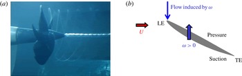
Figure 1(a) shows a picture taken from a water tunnel experiment where the forward mode of operation is visualized. A system of helical tip vortices and an axial hub vortex can be clearly seen. Note that the cross-sections of the tip vortices are very small. A cylindrical cross-section of a propeller blade is an airfoil; a schematic of the flow field around the airfoil is shown in figure 1(b). The flow approaching the airfoil is the vector sum of free stream and the flow induced by propeller rotation. The pressure difference generated between the pressure and suction sides of the blades creates net thrust and torque.
In the present work, we perform well-resolved LES of flow over marine propeller (DTMB 4381) at design advance ratio. The level of resolution and the length of the wake captured in the present work go beyond what has been reported in the literature, to the best of our knowledge. The entire evolution of propeller wake from near field to far field has been captured and explored in detail. The objectives of the present work are to: (i) evaluate the ability of LES to capture the complex evolution of propeller wakes, (ii) study the flow field in blade passage and the origin of loads on propellers, and (iii) understand the complex dynamics of propeller wake and its transition to instability. The paper is organized as follows. Simulation details including the numerical method, computational grid and boundary conditions are described in § 2. The simulations are validated against experimental data in § 3 and results are discussed in § 4. The mechanisms of propeller wake instabilities are discussed in § 5. Finally, the essential flow physics is summarized in § 6.
(a) Flow visualization of the forward mode at
 $J=0.3$
(Jessup et al.
Reference Jessup, Chesnakas, Fry, Donnelly, Black and Park2004) and (b) location of leading edge (LE), trailing edge (TE), and pressure and suction sides on blade section.

2 Simulation details
2.1 Numerical method
In LES, large scales are resolved by the spatially filtered Navier–Stokes equations, whereas the effect of small scales is modelled. Simulations are performed in a frame of reference that rotates with the propeller. The spatially filtered incompressible Navier–Stokes equations in the rotating frame of reference are formulated for the absolute velocity vector in the inertial frame as follows:
 $$\begin{eqnarray}\displaystyle \left.\begin{array}{@{}c@{}}\displaystyle \frac{\unicode[STIX]{x2202}\overline{u}_{i}}{\unicode[STIX]{x2202}t}+\frac{\unicode[STIX]{x2202}}{\unicode[STIX]{x2202}x_{j}}(\overline{u}_{i}\overline{u}_{j}-\overline{u}_{i}\unicode[STIX]{x1D716}_{jkl}\unicode[STIX]{x1D714}_{k}x_{l})=-\frac{\unicode[STIX]{x2202}\overline{p}}{\unicode[STIX]{x2202}x_{i}}-\unicode[STIX]{x1D716}_{ijk}\unicode[STIX]{x1D714}_{j}\overline{u}_{k}+\unicode[STIX]{x1D708}\frac{\unicode[STIX]{x2202}^{2}\overline{u}_{i}}{\unicode[STIX]{x2202}x_{j}\unicode[STIX]{x2202}x_{j}}-\frac{\unicode[STIX]{x2202}\unicode[STIX]{x1D70F}_{ij}}{\unicode[STIX]{x2202}x_{j}}\\ \displaystyle \frac{\unicode[STIX]{x2202}\overline{u}_{i}}{\unicode[STIX]{x2202}x_{i}}=0,\end{array}\right\} & & \displaystyle\end{eqnarray}$$
where
 $u_{i}$
is the inertial velocity in the inertial frame,
 $p$
is the pressure,
 $x_{i}$
are coordinates in the rotating non-inertial reference frame,
 $\unicode[STIX]{x1D714}_{j}$
is the angular velocity of the rotating frame of reference,
 $\unicode[STIX]{x1D708}$
is the kinematic viscosity,
 $\unicode[STIX]{x1D716}_{ijk}$
denotes the permutation tensor and the approximation
 $\overline{u_{i}\unicode[STIX]{x1D716}_{jkl}\unicode[STIX]{x1D714}_{k}x_{l}}\approx \overline{u}_{i}\unicode[STIX]{x1D716}_{jkl}\unicode[STIX]{x1D714}_{k}x_{l}$
is used. The terms containing
 $\unicode[STIX]{x1D714}_{j}$
in (2.1) take into account the effect of a rotating reference frame which is non-inertial.
 $\unicode[STIX]{x2202}/\unicode[STIX]{x2202}x_{j}(-\overline{u}_{i}\unicode[STIX]{x1D716}_{jkl}\unicode[STIX]{x1D714}_{k}x_{l})$
represents Coriolis acceleration whereas
 $-\unicode[STIX]{x1D716}_{ijk}\unicode[STIX]{x1D714}_{j}\overline{u}_{k}$
is representative of centrifugal acceleration. The overbar
 $\overline{(\cdot )}$
denotes the spatial filter and
 $\unicode[STIX]{x1D70F}_{ij}=\overline{u_{i}u_{j}}-\overline{u}_{i}\overline{u}_{j}$
is the subgrid stress. The subgrid stress is modelled by the Dynamic Smagorinsky Model (Germano et al.
Reference Germano, Piomelli, Moin and Cabot1991; Lilly Reference Lilly1992). The Lagrangian time scale is dynamically computed based on surrogate correlation of the Germano-identity error (Park & Mahesh Reference Park and Mahesh2009). This approach extended to unstructured grids has shown good performance for a variety of cases, including flow past a marine propeller in crashback (Verma & Mahesh Reference Verma and Mahesh2012).
Equation (2.1) is solved by a numerical method developed by Mahesh et al. (Reference Mahesh, Constantinescu and Moin2004) for incompressible flows on unstructured grids. The algorithm is derived to be robust without any numerical dissipation. It is a finite volume method where the Cartesian velocities and pressure are stored at the centroids of the cells and the face normal velocities are stored independently at the centroids of the faces. A predictor–corrector approach is used. The predicted velocities at the control volume centroids are first obtained and then interpolated to obtain the face normal velocities. The predicted face normal velocity is projected so that the continuity equation in (2.1) is discretely satisfied. This yields a Poisson equation for pressure which is solved iteratively using a multigrid approach. The pressure field is used to update the Cartesian control volume velocities using a least-square formulation. Time advancement is performed using an implicit Crank–Nicholson scheme. The algorithm has been validated for a variety of problems over a range of Reynolds numbers (see Mahesh et al. Reference Mahesh, Constantinescu and Moin2004).
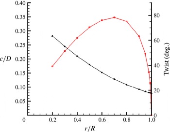
Chord (–▫–) and twist angle (–▵–) distribution for P4381 blades.

2.2 Propeller geometry, computational grid and boundary conditions
Simulations are performed for marine propeller DTMB 4381, which is a five-bladed, right-handed propeller with variable pitch, no skew and no rake. The geometric details of the propeller are reported in Bridges (Reference Bridges2004). The spanwise distribution of chord length and blade twist for this propeller is shown in figure 2.
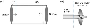
The domain size affects the propeller wake width and the pitch (e.g. Segalini & Inghels Reference Segalini and Inghels2014). Therefore, our computational domain (figure 3
a) is kept large enough to avoid any confinement effect. The computational domain used in the simulations is a cylinder of diameter
 $7.0D$
and length
 $10.0D$
, where
 $D$
is the diameter of the propeller disk. The blockage (
 $\unicode[STIX]{x1D716}=A_{d}/C$
, where
 $A_{d}$
is the disk area of propeller and
 $C$
is the area of test-section cross-section) is 0.082 in our simulations. As a rule of thumb, it is often assumed that if
 $\unicode[STIX]{x1D716}<0.1$
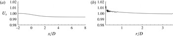
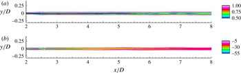
, the rotor wake is practically unconfined, and physical phenomena like wake instability are negligibly affected (Wilson Reference Wilson and Spera1994). The streamwise variation of the axial velocity is negligible (
 ${<}1\,\%$
) at
 $r/D=3.2$
as shown in figure 4(a).
The reference coordinate system is chosen such that the blades of the propeller are located at the origin and the flow is in the direction of positive
 $x$
. The domain extends
 $2D$
upstream and
 $8D$
downstream of the propeller. Preliminary simulations (not shown here) were performed with a longer domain in the upstream region with the inflow plane located at
 $6D$
upstream of the propeller. The radial variation of the axial velocity at
 $2D$
upstream of the propeller for this domain is negligible (
 ${<}1\,\%$
), as shown in figure 4(b). It was concluded that position of inflow at
 $2D$
upstream of the propeller will have negligible effect on propeller wake evolution. Hence, the present simulations can be considered devoid of any confinement effects.
(a) Computational domain and boundary conditions on domain boundaries, (b) boundary conditions on solid walls.

The variation of axial velocity (
 $U_{x}$
) in: (a) streamwise direction at
 $r/D=3.2$
and (b) radial direction at
 $x/D=-2$
. The variation of axial velocity from free stream is less than 1 %.

Free-stream velocity boundary conditions are specified at the inlet and the lateral far field boundaries. Convective boundary conditions are prescribed at the outflow. Since the velocities in the governing equations (2.1) are written in the inertial frame, boundary conditions on solid walls are also prescribed in the inertial frame. Thus, boundary conditions on the rotor part, blades and hub are specified as
 $\boldsymbol{u}=\unicode[STIX]{x1D74E}\times \boldsymbol{r}$
, while those on the shaft are prescribed as no-slip boundary conditions. A schematic of the computational domain and boundary conditions is shown in figure 3.
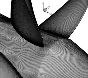
In the present work, simulations are performed using a computational grid which has 181 million control volumes consisting of only hexahedral cells. The unstructured grid for the propeller is shown in figure 5. The grid is designed carefully to capture all the essential features of the flow field. Any transverse cross-section on the shaft has 600 cells in the azimuthal direction. The radial cross-section of each blade has 324 cells along its circumference for the most part, except near the tip. There are at least 170 cells in the radial direction extending from root to tip on each blade. The grid is clustered close to all solid surfaces. Ten layers of hexahedral cells are extruded from the surface with a minimum wall-normal spacing of
 $0.0017D$
on blades and
 $0.00017D$
on hub and shaft surfaces to resolve near-wall flow features. A growth ratio of 1.02 is applied at all solid surfaces to transition from fine to coarser resolution away from the surface. The grid is refined in the wake region of the propeller to capture small scales. The entire grid is partitioned over 2048 processors and the simulations are performed with a time step of 0.001 unit, which corresponds to 10 668 computational time steps per rotation.
Close-up of surface mesh.

3 Validation
LES is performed at design advance ratio,
 $J=0.889$
at a Reynolds number
 $Re=894\,000$
. The value of
 $Re$
is chosen to match with the experimental conditions (Jessup et al.
Reference Jessup, Chesnakas, Fry, Donnelly, Black and Park2004; Jessup, Fry & Donnelly Reference Jessup, Fry and Donnelly2006). The advance ratio
 $J$
and Reynolds number
 $Re$
are defined as
 $$\begin{eqnarray}\displaystyle J=\frac{U}{nD},\quad Re=\frac{UD}{\unicode[STIX]{x1D708}}, & & \displaystyle\end{eqnarray}$$
where
 $U$
is the free-stream velocity,
 $n$
is the propeller rotational speed, and
 $D$
is the diameter of the propeller disk. Using the velocity magnitude experienced by the airfoil section of the blade and chord length, we also report a Reynolds number
 $$\begin{eqnarray}\displaystyle Re_{C}=\frac{U_{0.7}c_{0.7}}{\unicode[STIX]{x1D708}}, & & \displaystyle\end{eqnarray}$$
where
 $U_{0.7}$
and
 $c_{0.7}$
are the velocity magnitude and chord length at a radial location of
 $r/R=0.7$
. Here,
 $$\begin{eqnarray}\displaystyle U_{0.7}=\sqrt{U^{2}+(2\unicode[STIX]{x03C0}0.7Rn)^{2}}. & & \displaystyle\end{eqnarray}$$
The flow parameters of the simulations and experiments are listed in table 1. Here, OW and WT refers to the open water tow tank and water tunnel experiments, respectively (Jessup et al. Reference Jessup, Chesnakas, Fry, Donnelly, Black and Park2004, Reference Jessup, Fry and Donnelly2006).
The notation used throughout the paper is as follows. Thrust
 $T$
is the axial component of force and torque
 $Q$
is the axial component of the moment of force. Non-dimensional thrust coefficient
 $K_{T}$
and torque coefficient
 $K_{Q}$
are given by
 $$\begin{eqnarray}\displaystyle K_{T}=\frac{T}{\unicode[STIX]{x1D70C}n^{2}D^{4}}\quad \text{and}\quad K_{Q}=\frac{Q}{\unicode[STIX]{x1D70C}n^{2}D^{5}}, & & \displaystyle\end{eqnarray}$$
where
 $\unicode[STIX]{x1D70C}$
is the density of the fluid.
The computed mean
 $K_{T}$
and
 $K_{Q}$
are compared to the experimental results of Hecker & Remmers (Reference Hecker and Remmers1971) and Jessup et al. (Reference Jessup, Chesnakas, Fry, Donnelly, Black and Park2004, Reference Jessup, Fry and Donnelly2006), as shown in table 1. Jessup et al. (Reference Jessup, Chesnakas, Fry, Donnelly, Black and Park2004, Reference Jessup, Fry and Donnelly2006) report experiments conducted in a 36 in. water tunnel (WT) and open water towing-tank (OW), whereas Hecker & Remmers (Reference Hecker and Remmers1971) report experiments conducted in an open water towing-tank. LES results for
 $J=0.889$
(table 1) show good agreement with experiments for the mean value of thrust and torque coefficients. The measured values of loads is slightly smaller in the water tunnel, possibly due to tunnel effects. Our computed values of mean thrust and torque coefficients show good agreement with tow-tank data.
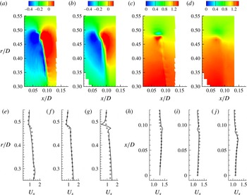
Phase-averaged blade wake: comparison between LES (a,c) and PIV (b,d); radial (a,b) and axial (c,d) velocities are compared. Axial velocity profiles are extracted and compared to PIV at streamwise (e–g) locations
 $x/D=0.06$
(e), 0.08 (f) and 0.1 (g); and radial (h–j) locations
 $r/D=0.35$
(h), 0.4 (i) and 0.45 (j). ——, LES; ▫, experiment (PIV). The values are normalized with
 $U$
.

 $J=0.889$
: flow parameters and mean values of thrust and torque coefficient.

The phase-averaged flow field in the blade wake is compared to PIV measurements (Chang, P. & Marquardt, M. 2016, private communication) in figure 6. The contours of computed radial and axial velocity fields are compared to the experimental data in figure 6(a–d). The thin vortex sheet in the blade trailing edge wake is nicely captured in the simulations which can be seen in both axial and radial velocity fields. The jump in radial velocity is sharper in results obtained from LES as compared to those of PIV, showing the level of resolution of the computational grid. The axial velocity contours also show better resolution of the tip vortex and blade wake in LES compared to that of the experiments having coarser spatial resolution. For more detailed comparison, profiles of axial velocity are shown at three streamwise locations (
 $x/D=0.06$
, 0.08 and 0.1) in figure 6(e–g) and also at three radial locations (
 $r/D=0.35$
, 0.4 and 0.45) in figure 6(h–j). Overall, the LES results show good agreement with the experiments.
Phase-averaged contours of eddy viscosity normalized with the molecular viscosity.

The phase-averaged eddy viscosity normalized with the molecular viscosity is shown in figure 7. The magnitude of eddy viscosity is small in the near field of the propeller wake, suggesting that the grid is resolving the flow field adequately. Hence, we expect that the behaviour of the flow fields described in the present work would remain unchanged if even finer grid resolution were employed.
 $J=0.889$
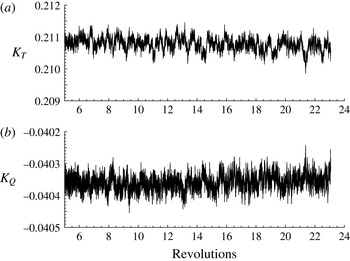
. Time history of unsteady loads on propeller: (a)
 $K_{T}$
and (b)
 $K_{Q}$
.

 $J=0.889$
. (a) Pressure and viscous contribution to thrust generated by the propeller and (b) PSD of unsteady loads,
 $K_{T}$
and
 $K_{Q}$
.

Pressure coefficient (
 $C_{p}$
) on propeller blade with streamlines at
 $J=0.889$
. (a) Pressure side and (b) suction side.

4 Results
4.1 Propeller loads
The time history of the thrust (
 $K_{T}$
) and torque (
 $K_{Q}$
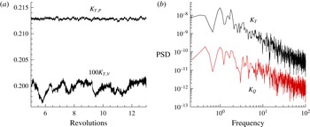
) coefficients are shown in figure 8. Unlike in off-design conditions like crashback (Jang & Mahesh Reference Jang and Mahesh2013), the deviation of loads from the mean is small at design conditions. The contribution of pressure and viscous forces to the thrust generated by the propeller is shown in figure 9(a). Note that the viscous force is negative. The magnitude of viscous contribution to thrust is compared to that of pressure. The pressure force is two orders of magnitude higher than that of the viscous force generated by the propeller.
The frequency spectra of the loads are computed by dividing the time history into a finite number of segments with 50 % overlap, applying a Hann window and rescaling to maintain the input signal energy. Each such segment is then transformed into the frequency domain by taking a fast Fourier transform (FFT). The power spectral density (PSD) is then averaged over all the segments. Figure 9(b) shows the PSD of the magnitude of
 $K_{T}$
and
 $K_{Q}$
as a function of non-dimensionalized frequency (
 $\text{rev}^{-1}$
). The unsteady loads on the propeller are broadband at design loading, as evident from the PSD of both
 $K_{T}$
and
 $K_{Q}$
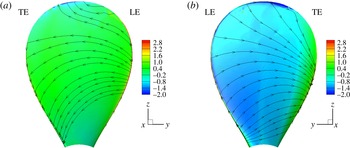
. Figures 10(a) and 10(b) shows the pressure coefficient (
 $C_{p}$
) with streamlines on the pressure and suction sides of propeller blades, respectively.
 $C_{p}$
is defined as
 $(p-p_{0})/0.5\unicode[STIX]{x1D70C}U^{2}$
, where
 $p$
is the pressure on the blade and
 $p_{0}$
is the free-stream pressure. The flow accelerates on the suction side of the blade for the most part, as evident from the lower pressure in that region. For both pressure and suction sides, the trailing edge region near the tip of the blade has the lowest pressure.
(a) Radial distribution of thrust coefficient: pressure side, –▵–; suction side, –▫– and (b) average circulation at
 $x=0.23R$
at design load.

In order to understand the contribution of different parts of blades to
 $K_{T}$
, the entire blade is split into 10 equal parts in the radial direction and the contribution to
 $K_{T}$
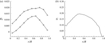
from each part is shown in figure 11(a) for both pressure and suction sides. Note that most of the thrust is generated from the region around the midspan of the blades. This is because the blade has the highest chord length in the midspan, and hence larger surface area for lift generation. The average spanwise loading on each blade can be computed from the circumferentially averaged azimuthal velocity similar to Jessup et al. (Reference Jessup, Chesnakas, Fry, Donnelly, Black and Park2004) as follows:
 $$\begin{eqnarray}G(r)=r\overline{U_{\unicode[STIX]{x1D703}}}(r)/Z,\end{eqnarray}$$
where
 $Z$
is the number of blades. The radial distribution of average spanwise loading is computed at
 $0.23R$
downstream of the propeller using (4.1), as shown in figure 11(b). The blade is gently loaded at the tip. This has an effect on the strength of the tip vortices generated by the propeller. A higher loading near the tip would generate a stronger and larger tip vortex. The strength of the vortices shed by the blade trailing edge is directly related to the radial gradient of circulation near that section of the blade. The average circulation for the propeller blades reaches a maximum at approximately
 $0.5R$
, followed by a decrease to zero at the tip. Thus, this propeller at design loading is expected to have stronger blade trailing edge wake as compared to propellers with heavy tip loading. This has major consequences in the dynamics of wake evolution, as discussed in the following sections.
Isocontour of
 $\unicode[STIX]{x1D706}_{2}$
coloured with axial velocity showing hub and tip vortices.

4.2 Axial evolution of propeller wake
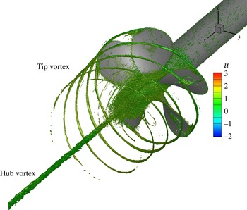
The propeller wake consists of five helical tip vortices (one originating from each blade) and an axial hub vortex. The coherent vortical structures in the propeller wake are visualized using the
 $\unicode[STIX]{x1D706}_{2}$
criterion (Jeong & Hussain Reference Jeong and Hussain1995).
 $\unicode[STIX]{x1D706}_{2}$
is the median of the three eigenvalues of
 $\unicode[STIX]{x1D64E}^{2}+\unicode[STIX]{x1D734}^{2}$
; here
 $\unicode[STIX]{x1D64E}$
and
 $\unicode[STIX]{x1D734}$
are respectively the symmetric and antisymmetric parts of the velocity gradient tensor
 $\unicode[STIX]{x1D735}\unicode[STIX]{x1D66A}$
. The isocontour of
 $\unicode[STIX]{x1D706}_{2}$
coloured with axial velocity is shown in figure 12. The structures at the inner radial location very near to the propeller are formed by the shedding of vorticity in the wake of individual blades. Figure 13 shows the instantaneous flow field in the
 $xy$
plane. The near field is dominated by coherent tip vortices and the blade trailing edge wake. These vortical structures become unstable and eventually break up to form the far wake. The vortex cores are seen clearly in contours of pressure field as a region of low pressure. The region inside the hub vortex has the lowest pressure, and hence is more susceptible to cavitation. The hub vortex region remains coherent with minor oscillations in the far field.
Instantaneous flow field in
 $xy$
plane: (a) axial velocity and (b) pressure. The axial velocity is normalized with
 $U$
, whereas the pressure field is normalized with
 $\unicode[STIX]{x1D70C}U^{2}$
.

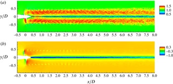
The flow field is phase-averaged over more than 15 rotations of the propeller after the transients die out, and analysed in the radial and axial planes from near to far field. Figure 14 shows the phase-averaged axial velocity and vorticity magnitude for the entire wake. Note the acceleration of the flow through the propeller, the contraction of the slipstream, and straining of the axial velocity in the near field. The axial velocity plot shows that the propeller wake has higher axial velocity than that of the free stream everywhere except in the hub vortex region, which is straight and confined to a thin region near axis. The vorticity field shows that the thin trailing edge wakes generated by the rotating blades break apart in the near field, generating a wake composed of hub and tip vortices along with smaller vortices which are generated by the breakup of blade trailing edge wakes. In the far field, the vortical structures present near the edge of the propeller wake weaken progressively until they are indistinguishable beyond
 $5D$
, as observed in figure 14(b).
Phase-averaged flow field in the
 $xy$
plane: (a) axial velocity and (b) vorticity magnitude. The axial velocity is normalized with
 $U$
. The vorticity magnitude is normalized using
 $U$
and
 $R$
.

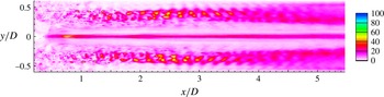
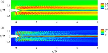
The pressure fluctuations and turbulent kinetic energy (TKE) are shown in the axial plane in figure 15. In the near field, the signature of the blade can be observed in both the pressure fluctuations and the TKE. The values of pressure fluctuation and TKE are negligible in the region of the stable tip vortex. In fact, there is a streamwise decay in TKE in the near field up to one diameter. This is due to decay of the shear layer of the blade wake, which is the source of TKE production in the near field. As soon as the tip vortex becomes unstable, both pressure fluctuations and TKE start increasing again. After roughly three diameters downstream of the propeller, the tip vortex breaks down completely, producing TKE. Subsequently, the radial extent of both pressure fluctuations and TKE spreads as we move further downstream. In the hub vortex, the TKE first decreases and then increases as we move downstream. The higher value of TKE in the hub vortex near the propeller is due to unsteadiness generated by flow separation on the hub. As we move axially downstream in the hub vortex, there is a sharp decrease in TKE, followed by an increase in TKE after the tip vortices destabilize. The tip vortex destabilization causes oscillations in the hub vortex, leading to the production of turbulence. This streamwise growth of TKE increases rapidly in the hub vortex once the tip vortices break down completely. This behaviour supports the hypothesis of Felli et al. (Reference Felli, Camussi and Di Felice2011) that there is a cause–effect relationship between the tip and hub vortex instability in propeller wakes.
Phase-averaged flow field in
 $xy$
plane: (a) pressure fluctuations and (b) turbulent kinetic energy. The flow field quantities are normalized appropriately using
 $\unicode[STIX]{x1D70C}$
and
 $U$
.

A series of transverse planes are extracted at nine streamwise locations, one upstream (
 $x/D=-0.2$
) and eight downstream (
 $x/D=0.2$
, 0.4, 0.6, 1, 1.5, 3, 5 and 7) of the propeller. The phase-averaged axial velocity, vorticity magnitude and turbulent kinetic energy are discussed below.
4.2.1 Flow upstream of propeller
The flow field of the propeller is shown at
 $x/D=-0.2$
(i.e.
 $0.2D$
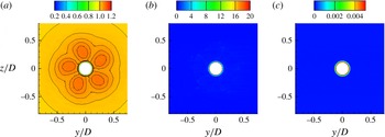
upstream of the propeller) in figure 16. The suction effect of the propeller can be seen in the axial velocity (figure 16
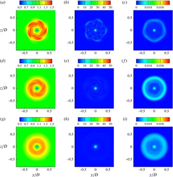
a). The vorticity and turbulent kinetic energy show that the propeller-induced perturbations do not produce significant turbulence in the upstream region. This shows that the propeller has negligible effect on its own inflow (i.e. the upstream region). All the vorticity and turbulence lie in the hub boundary layer, as seen in figures 16(b) and 16(c) respectively.
Upstream: phase-averaged axial velocity (a), vorticity magnitude (b) and TKE (c) at
 $x/D=-0.2$
. Isolines of axial velocity are also shown from 1 to 1.2 to illustrate the suction effect of the propeller. The flow field quantities are normalized appropriately using
 $\unicode[STIX]{x1D70C}$
,
 $R$
and
 $U$
.

4.2.2 Near wake
The evolution of propeller wake in the near field is shown in figure 17 at
 $x/D=0.2$
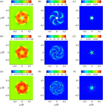
, 0.4 and 0.6. The vortex system comprising tip and hub vortices along with the thin vortex sheet shed by trailing edge of the blades are clearly seen. The visual inspection of instantaneous axial velocity and vorticity contours do not show any out-of-phase unsteadiness, suggesting that the trailing edge vortex sheet undergoes viscous dissipation and it is not an effect of phase-averaging. The progressive increase in the radial variation of pitch as we move downstream causes large deformation in vortical structures present in the wake, leading to the breakup of the tip vortices from their respective blade wakes. The bending in blade wake also brings the tip vortex close to the trailing edge wake of the next blade, thereby assisting in further distortion and destabilization. This behaviour was seen in the experiments of Felli et al. (Reference Felli, Guj and Camussi2008) as well. In their experiments, they varied the number of blades in the propeller from two to four and reported that this effect was more pronounced as the number of blades increased. The generation of turbulence is directly correlated with the destabilization of the vortices in the wake, as evident from the contours of the turbulent kinetic energy.
Near wake: phase-averaged axial velocity (a,d,g), vorticity magnitude (b,e,h) and TKE (c,f,i) at
 $x/D=0.2$
(a–c), 0.4 (d–f) and 0.6 (g–i). The flow field quantities are normalized appropriately using
 $\unicode[STIX]{x1D70C}$
,
 $R$
and
 $U$
.

A closer look at the axial velocity and vorticity shows breakup of the blade trailing edge vortex sheet. The stability and behaviour of vortex sheets have been explored by many authors in the past (Moore Reference Moore1974; Krasny Reference Krasny1986; Shelley Reference Shelley1992). Moore (Reference Moore1974) studied the evolution of an initially plane vortex sheet, which is similar to the wake generated by a fixed wing aircraft, and suggested that a finite vortex sheet with a tip vortex at its end undergoes a spiral roll-up. This in turn entrains some vorticity in the tip vortex, causing an instantaneous change in the velocity field at the locations of other vortices. These perturbations lead to the Kelvin–Helmholtz instability in the region between the tip vortex and the unstretched part of the vortex sheet. The breakup of blade trailing edge wake in the near field seems to follow a similar mechanism. However, in the present case we have an additional counter-rotating hub vortex at the other end of the blade trailing edge wake vortex sheet.
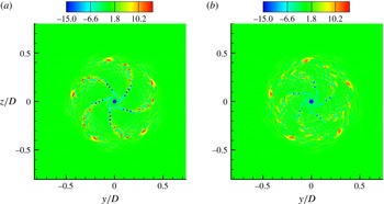
Figure 18 shows the axial component of vorticity fields at
 $0.4D$
and
 $0.6D$
downstream of the propeller. The spiral roll-up of the blade wake vortex sheet can be clearly seen. As seen in figure 18(b), the blade wake has undergone complete spiral roll-up, forming smaller vortical structures. These smaller vortex structures from the radially outward part of the blade interact with the tip vortices, which, among other things, dictate the evolution of the propeller wake in the intermediate field.
Roll-up in blade trailing edge wake. Axial component of vorticity at
 $x/D=0.4$
(a) and
 $0.6$
(b). The values are normalized appropriately using
 $U$
and
 $R$
.

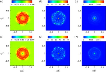
Intermediate wake: phase-averaged axial velocity (a,d), vorticity magnitude (b,e) and TKE (c,f) at
 $x/D=1$
(a–c) and 1.5 (d–f). The values are normalized appropriately using
 $U$
and
 $R$
.

It can be seen that, although the tip vortices have broken apart from their respective blade wake, still they are stable, which is supported by the lack of turbulence in the region of tip vortices. In conclusion, the near field of the propeller wake is characterized by the progressive distortion, viscous dissipation and eventual breakup of thin blade trailing edge wakes, leading to separation of tip vortices from their respective blade wakes.
4.2.3 Intermediate wake
The intermediate wake is characterized by the growth of the instabilities in tip vortices. The wake becomes increasingly unstable as we go downstream, as evident from the plots of turbulent kinetic energy (figure 19) from
 $x/D=1{-}1.5$
. The flow field at
 $x/D=1.5$
shows the weakening of tip vortex signatures as compared to
 $x/D=1$
. The vorticity plot at
 $x/D=1.5$
(figure 19
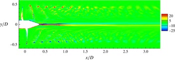
e) shows additional vortical structures along with the tip vortices. The possible mechanism of their formation is described as follows. As described in the previous section (§ 4.2.2), the blade trailing edge wake, which is a thin vortex sheet, breaks up into smaller fragments (figure 17). Figure 20 shows the
 $z$
-component (out of plane) of vorticity. It can be seen that the tip vortices and hub vortex are of opposite sign, whereas the tip vortex and trailing edge wake of the preceding blade are of same sign, hence they attract each other. The tip vortex, being stronger, pulls the weak blade wake vortices closer to its own axial plane as the wake evolves from the near field to the intermediate field. These vortical structures are responsible for the onset of turbulence and pressure fluctuation generation near the edge of the wake seen earlier in figure 15.
It should be noted that the mechanism of the mutual-inductance mode of instability explained here is fundamentally different than what was observed and described by earlier authors. Di Felice et al. (Reference Di Felice, Di Florio, Felli and Romano2004) and Felli et al. (Reference Felli, Di Felice, Guj and Camussi2006) explained that the interaction between the tip vortex and the trailing wake of the adjacent blade in the same transverse plane cause the tip vortex to break apart from its trailing edge blade wake. Felli et al. (Reference Felli, Camussi and Di Felice2011) performed detailed experiments with propellers and noted that the transition to instability may be correlated more to spiral-to-spiral interaction than to the complete development of trailing wake roll-up. They explained that the mutual inductance between the adjacent tip vortices causes the adjacent tip vortex spirals to roll-up around each other, causing leap-frogging, particularly for a four-bladed propeller due to proximity of tip vortex spirals. However, in the present case, we see the mutual inductance between the tip vortex and the adjacent blade wake in the axial plane. The possible reason for the difference in the mechanism of mutual inductance between the present case and those reported earlier in the literature is the blade geometry itself. The blade geometry of the propeller used in the experiments of Di Felice et al. (Reference Di Felice, Di Florio, Felli and Romano2004), Felli et al. (Reference Felli, Di Felice, Guj and Camussi2006) and Felli et al. (Reference Felli, Camussi and Di Felice2011) is such that it is highly loaded at the tip, thus shedding strong tip vortices. The blades also have a forward rake and slight skew. On the other hand, the propeller used in the present work is without any skew and rake, and is nominally loaded (see figure 11 b) at the tip, thus shedding a relatively weaker tip vortex and a stronger blade trailing edge wake at design conditions.
Hence, although the mutual-inductance mode of instability is dominant in wake destabilization, the actual mechanism is dependent on the geometry as well as the operating condition. Propellers which are highly loaded at the tip will produce stronger tip vortices, causing spiral-to-spiral interaction of tip vortices to be the dominant mechanism of wake instability, as opposed to the propellers with nominally loaded tip, where the interaction between the blade wake and adjacent tip vortices in both axial and transverse planes is the dominant mechanism for the propeller wake instabilities.
Close-up view of the
 $z$
-component of vorticity in the
 $xy$
plane. The values are normalized appropriately using
 $U$
and
 $R$
.

Far wake: phase-averaged axial velocity (a,d,g), vorticity magnitude (b,e,h) and TKE (c,f,i) at
 $x/D=3$
(a–c), 5 (d–f) and 7 (g–i). The values are normalized appropriately using
 $U$
and
 $R$
.

4.2.4 Far wake
The evolution of propeller wake in far field is shown in figure 21. The contours of phase-averaged axial velocity, vorticity and turbulent kinetic energy contours are plotted at
 $x/D=3$
, 5 and 7 downstream of the propeller. Once the tip vortices destabilize completely in the intermediate wake, the wake evolves as a shear layer in both the axial and azimuthal directions. These shear layers are susceptible to shear layer instabilities. There are minor signs of the Kelvin–Helmholtz instabilities in both axial (figure 14
a) and azimuthal (figure 21
a) shear layers around
 $x=3D$
. The turbulent kinetic energy plots suggest generation of turbulence in the outer edge of the wake as well as the hub vortex core. The region between the outer edge of wake and the edge of hub vortex is comparatively less turbulent. This region seems to possess some flow structures which look like a mild signature of propeller blades mainly in the axial velocity field. This could be related to the centrifugal instability of the propeller wake, which acts as a swirling jet of fluid around an axial hub vortex. The vorticity plots suggest that all the tip vorticity is dissipated and most of the vorticity lies in the hub vortex (figure 21
e).
4.3 Flow in blade passage
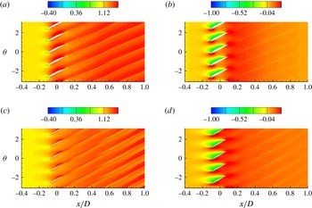
The phase-averaged axial velocity and pressure field in the vicinity of the propeller are plotted in figure 22 for two cylindrical cut planes at
 $r/R=0.4$
and 0.7, showing flow field details at root and midspan sections of propeller blades, respectively. The flow is attached at both these radial locations. Acceleration of flow can be seen in the blade passage, which creates a pressure difference across the blade sides, generating net force and torque. The wake of blades has trailing edge vortices which give the appearance of streaks in the plots. The spreading of wake of airfoil sections of blades can also been seen here. The blade wakes have larger spreading near the midspan section as compared to the blade root. The spreading in the phase-averaged velocity field is the result of unsteadiness in the flow field which increases as we move downstream.
Phase-averaged axial velocity (a,c) and pressure (b,d) in the
 $x\unicode[STIX]{x1D703}$
plane at:
 $r/R=0.4$
(a,b) and
 $r/R=0.7$
(c,d). The axial velocity and pressure are normalized with
 $U$
and
 $\unicode[STIX]{x1D70C}U^{2}$
respectively.

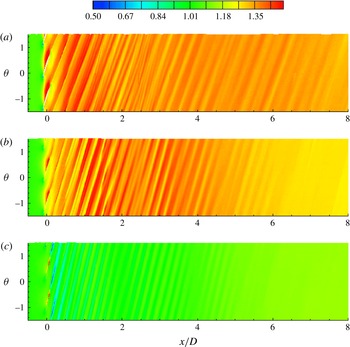
Phase-averaged axial velocity in the
 $x\unicode[STIX]{x1D703}$
plane at
 $r=0.4R$
(a),
 $0.7R$
(b) and
 $0.95R$
(c). The values are normalized with
 $U$
.

Phase-averaged vorticity magnitude in the
 $x\unicode[STIX]{x1D703}$
plane at
 $r=0.4R$
(a),
 $0.7R$
(b) and
 $0.95R$
(c). The values are normalized appropriately using
 $U$
and
 $R$
.

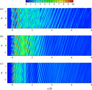
Phase-averaged turbulent kinetic energy in the
 $x\unicode[STIX]{x1D703}$
plane at
 $r=0.4R$
(a),
 $0.7R$
(b) and
 $0.95R$
(c). The values are normalized appropriately using
 $U$
.

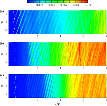
The phase-averaged axial velocity (figure 23), vorticity magnitude (figure 24) and turbulent kinetic energy (figure 25) are plotted in the
 $x\unicode[STIX]{x1D703}$
plane at three radial distances of 40 %, 70 % and 95 % radius from the axis for the entire wake. Stripes of low and high velocity are distinct in the near field. The wakes from the adjacent blades interact with each other as they evolve downstream. Such interactions are particularly stronger for a five-bladed propeller, as the blade wakes are closer to each other as compared to say, two-bladed propellers. The spatial oscillations in the blade wakes causes meandering and smearing, as observed in the plots of phase-averaged flow field quantities. Such effects are very prominent between
 $1<x/D<3$
. Note that there is lack of distinct low- and high-velocity regions at
 $0.95R$
radially outward from axis. This is because of low loading and chord length at this radial location. Nevertheless, there is shedding of tip vortices, whose effect is seen in the near field, but then the wake undergoes streamtube contraction. Also, the slope of the stripes depends on blade twist and loading conditions. As blade twist (figure 2) and approach velocity vary with varying radial location, the slope of the stripes varies radially. This slope is smallest near the root, and increases radially outward from axis. Blade wakes contain vorticity, which form stripes in vorticity plots as well (figure 24). These striped patterns are clear even at
 $0.95R$
, which is due to high velocity gradients in this region. Wake contraction effects are visible here as well. There appear to be stripes of vorticity at
 $r/R=0.7$
around
 $x/D=2$
. This is formed by the process of entrainment of the small vortical structures formed by the breakup of blade trailing edge wakes by the tip vortices, which happens in the intermediate wake, as discussed in section § 4.2.3. The transition of blade wakes to instability can be visualized by turbulent kinetic energy (figure 25). The turbulence is produced near the root first. This is because of viscous diffusion of the thin blade wake. This onset of turbulence production moves downstream as we move radially outwards. Most of turbulence is situated in the far wake, where all the structures are already broken up.
4.4 Azimuthal-averaged propeller wake
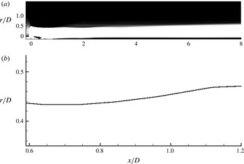
In order to analyse the propeller wake, the phase-averaged flow field is further averaged in the azimuthal direction to obtain azimuthal-averaged flow features. The inception of tip vortex instabilities creates oscillations in the envelope of the wake. Felli et al. (Reference Felli, Camussi and Di Felice2011) plotted the standard deviation image calculated over 1000 snapshots in time, which they used to identify the location of instabilities in hub and tip vortices. Figure 26(a) shows the azimuthal-averaged wake envelope of the propeller, where dark shade shows the region where the axial velocity is higher than the free-stream velocity. The line tracing the wake envelope is extracted, as shown in figure 26(b), where it is plotted in the region of the near field. The method used by Felli et al. (Reference Felli, Camussi and Di Felice2011) is applied to obtain the axial location where the tip vortex destabilizes, which is at
 $x/D=0.8$
.
(a) The envelope of the propeller wake and (b) the line tracing the envelope of the propeller wake in the near field.

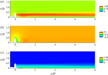
Azimuthal-averaged velocity components are shown in figure 27. In the near field, a low-axial-momentum region is seen, which is created by flow separation on the hub. The radial velocity
 $U_{r}$
is very small everywhere in the domain, except in the vicinity of blade, where it is negative. This is because the propeller entrains fluid from its surrounding and pushes it downstream. The major difference between streamwise velocity and azimuthal velocity fields is that the maximum of azimuthal velocity at any streamwise location lies in hub vortex, whereas that of streamwise velocity lies around the midspan of the propeller. The higher axial velocity around the midspan of the propeller leads to faster advection of blade wake compared to the tip vortices. This brings the tip vortex of a blade very close to the trailing edge wake of the previous blade (see figure 14). The radial decrease in azimuthal velocity outside the hub vortex makes the blade trailing edge wake rotate faster than the tip vortices which are located at the edge of propeller wake. This leads to an increase in bending of the blade wakes (see figure 17). All of these phenomena assist in the mutual-inductance mode of instabilities which will be discussed in § 5.
Azimuthal-averaged velocity components in the
 $xr$
plane: (a) axial, (b) radial and (c) azimuthal. The values are normalized with
 $U$
.

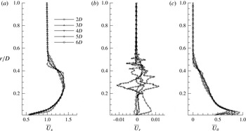
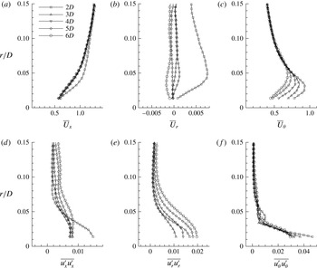
Profiles of velocity components are extracted at five locations from
 $2D$
to
 $6D$
downstream of the propeller, as shown in figure 28. Wake contraction in the near field leads to a smaller wake width as compared to the propeller radius at
 $2D$
. It is interesting to see that all the profiles overlap up to
 $r=0.2R$
except the profile at
 $x=2D$
in the axial velocity. This means the streamwise variation of axial velocity is negligible for
 $x>3D$
, i.e. in the far field in the inner part of the propeller wake. It can also be seen that as the wake evolves downstream, the profile becomes smoother mainly near the edge of the wake, which signifies diffusion and expansion of the wake as one moves from
 $2D$
to
 $6D$
.
Azimuthal-averaged profile of velocity components: (a) axial, (b) radial and (c) azimuthal. The values are normalized appropriately with
 $U$
.

It is interesting to see that the mean axial velocity in the propeller wake is higher than the free stream everywhere except in the hub vortex. The azimuthal velocity is zero outside the propeller wake. The fluid column has an angular momentum which decays as we move radially outwards. Thus, the propeller wake can be thought of as a superimposition of swirling velocity along with a high axial momentum surrounding the wake of hub which has an axial momentum deficit.
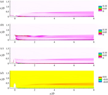
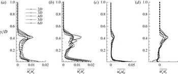
Figure 29 shows azimuthal-averaged mean square velocity fluctuation components. The profiles are also extracted at five locations from
 $2D$
to
 $6D$
downstream of the propeller (figure 30). The streamwise and azimuthal components grow after the tip vortices become unstable, whereas the radial fluctuations are very high in the region of stable tip vortex. A possible reason can be mutual interaction between adjacent spirals of helical tip vortices which are strongest in the near field. The radial extent of velocity fluctuations grow for all components as we move downstream after the tip vortices become unstable. This is observed clearly in the plots of the radial profile of mean square velocity components (figure 30). The axial velocity fluctuations are high in the region of the tip vortices (edge of wake) and hub vortex (near axis). The axial velocity fluctuations are nearly constant in the entire wake except in hub and tip vortices. The axial velocity fluctuations remain fairly constant in the hub vortex beyond
 $x=3D$
. The radial velocity fluctuations show a remarkably different behaviour. The radial velocity fluctuations in the hub vortex decay from
 $2D$
to
 $3D$
, followed by a subsequent growth. This can be explained as follows. The flow separation on the hub creates a region of high turbulence near the end of the hub. These high fluctuations in all velocity components undergo viscous dissipation up to
 $3D$
. Until
 $x=3D$
, the tip vortices break down completely, which disturbs the equilibrium of the system containing hub and tip vortices. This causes the hub vortex to oscillate in the radial direction, thus increasing fluctuations in the radial component of the velocity field. Outside the hub vortex, two peaks are observed in the radial velocity fluctuation profile. These peaks flatten out in the far wake. There is negligible fluctuation in the azimuthal velocity component except in the region of hub and tip vortices. The Reynolds stress component
 $\overline{u_{x}^{\prime }u_{r}^{\prime }}$
shows a higher value in the vicinity of the hub and the wake edge after destabilization of the tip vortices. The roll-up of blade trailing edge wake in the near wake also increases the value of
 $\overline{u_{x}^{\prime }u_{r}^{\prime }}$
, as can be seen in the near field. The profiles of
 $\overline{u_{x}^{\prime }u_{r}^{\prime }}$
show that its value is negative in the hub vortex region, where it is positive everywhere else in the wake.
Azimuthal-averaged mean square velocity fluctuations in the
 $xr$
plane: (a) axial (
 $\overline{u_{x}^{\prime }u_{x}^{\prime }}$
), (b) radial (
 $\overline{u_{r}^{\prime }u_{r}^{\prime }}$
), (c) azimuthal (
 $\overline{u_{\unicode[STIX]{x1D703}}^{\prime }u_{\unicode[STIX]{x1D703}}^{\prime }}$
) and (d) Reynolds stress (
 $\overline{u_{x}^{\prime }u_{r}^{\prime }}$
). The values are normalized with
 $U^{2}$
.

Azimuthal-averaged profile of mean square velocity fluctuations: (a) axial (
 $\overline{u_{x}^{\prime }u_{x}^{\prime }}$
), (b) radial (
 $\overline{u_{r}^{\prime }u_{r}^{\prime }}$
), (c) azimuthal (
 $\overline{u_{\unicode[STIX]{x1D703}}^{\prime }u_{\unicode[STIX]{x1D703}}^{\prime }}$
) and (d) Reynolds stress (
 $\overline{u_{x}^{\prime }u_{r}^{\prime }}$
). The values are normalized with
 $U^{2}$
.

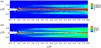
Azimuthal-averaged pressure (a), mean square pressure fluctuation (b) and turbulent kinetic energy (c) in the
 $xr$
plane. The values are normalized appropriately using
 $\unicode[STIX]{x1D70C}U^{2}$
.

The azimuthal-averaged Reynolds stress is shown in figure 29(d). As evident from the plot, Reynolds stress is maximum near the edge of the wake from
 $x/D=1.5$
to 3.5, after which it grows rapidly in the radial as well as the streamwise direction. Thus, this is the region of intense turbulent production which can be seen in figure 15(b). The radial profiles at five streamwise locations downstream of the propeller are also plotted in figure 30(d). The radial expansion of the region of high Reynolds stress is clearly evident. Also, the peak of the Reynolds stress profile decreases in the far wake, as seen in the profiles from 4
 $D$
to 6
 $D$
.
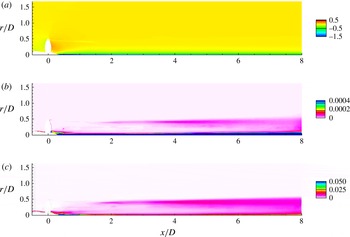
The azimuthal-averaged pressure and mean square pressure fluctuations are shown in figures 31(a) and 31(b) respectively. The low pressure cores of tip vortices appear as a streak here because of averaging in the azimuthal direction. The hub vortex is the region of low pressure and is therefore most susceptible to cavitation. There is negligible streamwise gradient in pressure field beyond
 $x=3D$
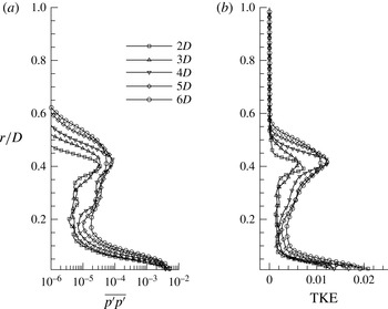
i.e. in the far wake. The pressure fluctuation shows a trend similar to the axial and azimuthal velocity fluctuations as discussed earlier. The region inside the hub vortex contains large pressure fluctuations. This is also evident from the profiles of pressure fluctuations as shown in figure 32(a). The radial extent of high-pressure fluctuations near the edge of the wake increases as the wake expands in the far field. A small region of high-pressure fluctuation is seen in the near field at
 $(x/D,r/D)=(0.5,0.2)$
. This seems to be the effect of oscillations in the blade trailing edge wake near the root of blades in the near field. Overall, the pressure field suggests that the propeller wake away from the blade evolves from the near field to the far field in a nominal zero pressure gradient environment in the axial direction and, hence, the far wake in particular can be treated as a column of fluid swirling around an axial hub vortex such that the net axial linear momentum and azimuthal angular momentum are conserved. Hence, the possibility of existence of a self-similar solution in the far wake exists.
Azimuthal-averaged profile of mean square pressure fluctuation (a) and turbulent kinetic energy (b). The values are normalized using
 $\unicode[STIX]{x1D70C}U^{2}$
.

Figure 31(c) shows azimuthal-averaged turbulent kinetic energy. The turbulent kinetic energy is high near the end of the hub because of fluctuations caused by flow separation on the hub. The magnitude of turbulent kinetic energy decreases rapidly as we move downstream in the near-axis region in the near wake. There is negligible turbulence near the edge of the wake in the near field due to stable tip vortices, as already discussed earlier. The turbulent kinetic energy grows both near the axis and near the edge of the propeller wake beyond
 $x/D=1.5$
following the onset of instabilities in the tip vortices. The turbulent kinetic energy grows both in magnitude and radial extent moving further downstream. In general, the turbulent kinetic energy increases in the far wake, as seen in radial profile of TKE (figure 32
b).
Hub vortex: phase-averaged axial velocity (a) and axial vorticity (b) in the
 $xy$
plane. The values are normalized appropriately using
 $U$
and
 $R$
.

4.5 The hub vortex
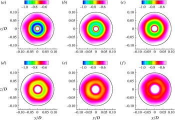
The hub vortex is an important component of propeller wake which dominates the flow field. The phase-averaged axial velocity and axial vorticity in the hub vortex region are shown in figure 33. Figure 34 shows the phase-averaged azimuthal (swirl) velocity at multiple axial locations from 2 to 7 diameters downstream of the propeller. A circle of radius
 $0.1D$
centred on the axis of propeller is also shown for reference. Both these figures confirm that the hub vortex remains coherent throughout the simulated domain. However, minor oscillations about the propeller axis can be observed, mainly beyond
 $x/D=4$
(figure 34
c–f). Note that the hub vortex is non-axisymmetric. This deviation from axisymmetry increases in the far wake. The large values of velocity and pressure fluctuations observed earlier in the hub vortex are the result of azimuthal-averaging of this non-axisymmetric hub vortex.
Hub vortex: phase-averaged azimuthal (swirl) velocity at
 $x/D=2$
(a), 3 (b), 4 (c), 5 (d), 6 (e) and 7 (f) downstream of the propeller. The black solid line is a circle of radius
 $0.1D$
centred on the axis of the propeller.

The radial profiles of azimuthal-averaged velocity and mean square velocity fluctuations discussed earlier (§ 4.4) are reproduced in figure 35 with the
 $y$
axis zoomed-in to focus in the region of the hub vortex.
The flow field in the hub vortex region shows large axial and azimuthal (swirl) velocities, whereas the radial velocity is negligible. Note that the variation in axial velocity is negligible in the far field, whereas the swirl velocity keeps decreasing with increasing streamwise distance from the propeller. The large swirl velocity is important to the stability of the propeller wake, as concluded by Okulov & Sørensen (Reference Okulov and Sørensen2007), who modelled the hub vortex field by assigning a vorticity distribution. They showed that the inclusion of a simple Rankine vortex (to model the hub vortex field) to the Joukowski model could predict the rotor wake rather accurately. Thus, the swirl velocity induced by the hub vortex field stabilizes the otherwise unconditionally unstable Joukowski model. Although the hub vortex field described in the present work is too complicated to be modelled as a simple Rankine vortex, the observed trend in the present work is consistent with the analysis of Okulov & Sørensen (Reference Okulov and Sørensen2007). The minor oscillations in the hub vortex as discussed earlier cause an increase in the azimuthal-averaged fluctuations, as evident in figure 35(d–f). These profiles also show a rapid decrease in fluctuations away from the axis in the hub vortex region.
Azimuthal-averaged profile of components of velocity (a–c) and mean square velocity fluctuations (d–f) at locations
 $x/D=2$
, 3, 4, 5 and 6. The values are normalized appropriately using
 $U$
.

5 Mechanisms of propeller wake instabilities
The mutual-inductance mode of instability has been suggested to drive the transition to unstable wake in rotors. Experimental investigation of propeller wake by Felli et al. (Reference Felli, Camussi and Di Felice2011) for a variety of operating conditions and number of blades indicates that the mutual-inductance mode of instability dominates the wake evolution. Nevertheless, short-wave and long-wave mode of instabilities first predicted by Widnall (Reference Widnall1972) were also observed in their experiments. A number of recent works on wind turbine wakes have also established the dominance of the mutual-inductance mode as the prime mechanism for driving the rotor wake instabilities (Sherry et al. Reference Sherry, Nemes, Lo Jacono, Blackburn and Sheridan2013a ,Reference Sherry, Sheridan and Lo Jacono b ; Sarmast et al. Reference Sarmast, Dadfar, Mikkelsen, Schlatter, Ivanell, Sørensen and Henningson2014). Although the general characteristics of propeller and wind turbine wakes are same, i.e. similar hub (and/or root) and tip vortices, there are some important fundamental differences.
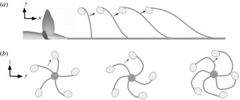
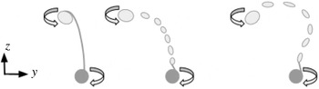
Schematic diagram showing mutual interaction between the tip vortex and the adjacent blade wake in the
 $xy$
(a) and
 $yz$
(b) planes. The flow is from left to right in the
 $xy$
plane (a). The axial evolution is shown in the
 $yz$
plane (b) from left to right. The sense of rotation is clockwise in this view.

Wind turbine rotors are designed to extract energy from the flow and, hence, the wind turbine wake has lesser momentum in comparison to free stream, unlike propeller wake, which pushes flow downstream increasing momentum. Therefore, the wind turbine wake has maximum axial velocity near the edge of the wake. This makes the tip vortex move faster than the weak and thin blade trailing edge wakes. These blade wakes dissipate rapidly in the near field, whereas the tip vortices come close to each other, making them susceptible to the mutual-inductance mode of instability through a so-called leap-frogging mechanism (Lignarolo et al. Reference Lignarolo, Ragni, Krishnaswami, Chen, Ferreira and Van Bussel2014, Reference Lignarolo, Ragni, Scarano, Ferreira and van Bussel2015). This leap-frogging mechanism was also observed by Felli et al. (Reference Felli, Camussi and Di Felice2011), mainly for higher loading conditions for four-bladed propeller. As expected, this mechanism is commonly observed for those rotor wakes which have small spiral-to-spiral distance. Thus, increasing the number of blades or decreasing the advance ratio facilitates the leap-frogging mechanism.
In marine propellers, however, there are other possible mechanisms of the mutual-inductance mode of instabilities. The interaction between the tip vortex and the adjacent blade wake is highly likely, mainly for marine propellers which have higher number of blades. This mechanism is particularly preferred when the spiral-to-spiral distance is large (large advance ratio), i.e. the propeller is not highly loaded. Figure 36 illustrates this mechanism of mutual inductance in both the axial (
 $xy$
) and transverse (
 $yz$
) planes.
Another important physical phenomenon which is active in the propeller wake is spiral roll-up of the blade trailing edge vortex sheet, as mentioned in § 4.2.2. This phenomenon is responsible for detaching the tip vortices from the blade trailing edge wake after complete roll-up and formation of smaller fragments of the trailing edge wake, which eventually dissipate to form the far wake, as described by Joukowski (Reference Joukowski1912), consisting of only tip and hub vortices. However, as observed by Felli et al. (Reference Felli, Camussi and Di Felice2011), mutual interference between consecutive spirals of the tip vortices were much more important than complete development of the trailing edge wake roll-up. The present case seems different from what has been observed in earlier experiments. As already pointed out earlier, the propeller used in the present simulations is designed to have weaker tip vortices as compared to the propeller used by Felli et al. (Reference Felli, Camussi and Di Felice2011) and others. As the mutual inductance between tip vortices is not strong, the trailing edge wake takes time to undergo roll-up in both the axial
 $xy$
and transverse
 $yz$
planes. The schematic of roll-up in the
 $yz$
plane is shown in figure 37.
Schematic diagram showing blade trailing edge vortex sheet roll-up in the
 $yz$
plane. The arrows show the sense of rotation of the vortices. The axial evolution is shown in the figure as we go from left to right.

Schematic diagram showing blade trailing edge vortex sheet roll-up coupled with mutual interaction between the tip vortex and the adjacent blade wake in the transverse
 $xy$
plane. Flow is from left to right. The arrows show the mutual interactions.

The analysis of Okulov & Sørensen (Reference Okulov and Sørensen2007) suggested that the occurrence of concentrated tip vortices is the consequence of complete roll-up of the blade trailing edge wake, which subsequently triggers instabilities. This implies that the downstream location where the propeller wake becomes unstable should be independent of the number of blades as long as the tip vortex intensity is identical. However, Felli et al. (Reference Felli, Camussi and Di Felice2011) observed that the downstream distance where the propeller wake becomes unstable depends on the number of blades despite having identical tip vortex intensity. They argued that the formation of concentrated tip vortices is more affected by the trailing edge wake of the blade and the tip vortex of the previous blade.
The propeller wake simulated in the present work shows all of the above-mentioned phenomenon in some form or other, but the mutual inductance between the rolled-up trailing edge wake and the tip vortices dominates the evolution of the propeller wake from the near field to the far field. Figure 38 illustrates this mechanism. The rolling-up of trailing edge wake begins very close to the propeller in the near field. The progressive bending in the
 $yz$
plane (figure 37) and slanting in the
 $xy$
plane facilitates the mutual interaction between smaller vortical structures generated by blade wake roll-up and the tip vortices in the intermediate wake. This mechanism, where the roll-up of blade trailing edge wake generates concentrated vortices which subsequently interact with the tip vortices causing wake instability, is different from that observed in experiments (Di Felice et al.
Reference Di Felice, Di Florio, Felli and Romano2004; Felli et al.
Reference Felli, Camussi and Di Felice2011) and is not reported in the literature to the best of our knowledge. This mechanism is expected to be dominant for propellers which generate weaker tip vortices but have a higher number of blades.
6 Summary
The complex dynamics of rotor wakes have been of interest for many decades because of their use in several engineering applications. LES is becoming increasingly popular in recent years to capture complex flow physics which is otherwise impossible to capture (Mahesh et al. Reference Mahesh, Kumar, Gnanaskandan and Nitzkorski2015). In this paper, we use well-resolved LES to understand the details of the complex dynamics of the wake of a five-bladed marine propeller at design advance ratio. Care has been taken to resolve important small scales as well as the entire evolution of the propeller wake from the near field to the far field without any confinement effects, which is known to affect the propeller wake in general and tip vortex dynamics in particular.
Phase-averaged and azimuthal-averaged flow fields are used to characterize the evolution of the propeller wake from the near field to the far field. In the near field, the thin blade trailing edge wakes, which are generated because of spanwise variation of loading on the propeller blades, undergo dissipation and Kelvin–Helmholtz destabilization, leading to roll-up in both the axial and transverse planes. This leads to the formation of small vortical structures. Although the tip vortices break apart from the blade trailing edge wakes, they still remain stable in the near field. Eventually, these tip vortices destabilize due to strong mutual induction between them and small vortical structures formed as a result of roll-up, causing them to oscillate. The nature of mutual inductance is such that the interaction between the blade trailing edge wake and the tip vortex of the adjacent blade is stronger than the spiral-to-spiral (Felli et al. Reference Felli, Camussi and Di Felice2011) and tip vortex-adjacent blade wake interactions (Di Felice et al. Reference Di Felice, Di Florio, Felli and Romano2004) observed in earlier experiments.
It is argued that the preferred mechanism of the mutual-inductance mode of instabilities in rotor wakes depends on the blade geometry and operating conditions. A propeller designed to have a strong tip vortex will have stronger mutual interactions between adjacent tip vortices. This mechanism is further aided by a lower advance ratio and a higher number of blades because of the decreased spiral-to-spiral distance. On the other hand, a propeller with relatively weaker tip loading will have weaker mutual interactions between the tip vortices. A lower advance ratio further delays this mechanism due to a higher spiral-to-spiral distance. Hence, the blade trailing edge wake completes its spiral roll-up, forming discrete vortical structures. These vortices, being of smaller magnitude than tip vortices, get pulled towards the edge of wake by the tip vortices as the wake evolves in the intermediate field. After becoming unstable, the oscillating vortical structures produce turbulence in the wake. In the far field, the wake can be thought of as a region of high axial and swirl velocity around an oscillating hub vortex. The wake becomes increasingly axisymmetric as it evolves in the far field, where it appears as a fluid mass swirling around an axial hub vortex. At design advance ratio, the hub vortex remains coherent up to the length of wake captured in our simulations (
 $8D$
). It undergoes some minor oscillations after destabilization of the tip vortices, as evident in the increase in radial velocity fluctuations. Almost all of the pressure fluctuations lie in the hub vortex. The further evolution of the far wake may follow a self-similar behaviour. The axial and azimuthal shear layers in the far wake are susceptible to Kelvin–Helmholtz instabilities.
Acknowledgements
This work was supported by the United States Office of Naval Research (ONR) under ONR grant N000141410289, with Dr K.-H. Kim as technical monitor. The computations were made possible through the computing resources provided by the US Army Engineer Research and Development Center (ERDC) in Vicksburg, Mississippi on the Cray XE6, Copper and Garnet of the High Performance Computing Modernization Program (HPCMP). The authors also acknowledge the Minnesota Supercomputing Institute (MSI) at the University of Minnesota for providing resources that contributed to the research reported in this paper. We are grateful to Dr P. Chang and Dr M. Marquardt at Naval Surface Warfare Center Carderock Division (NSWCCD) for providing us with experimental PIV data used for validation purposes.