2.1 Devon Island records

In 1972 and 1973 two bore holes were drilled 27 m apart on the Devon Island ice cap (Table I). Both holes are about 900 m from the summit ridge and 7.5 km west of the highest surface elevation of the ice cap. Seasonal δ(¹⁸O) oscillations die out after only 14 cycles due to diffusion in the firn.

Table I

Drill Sites

The δ(¹⁸O) samples were cut initially according to a theoretical time scale. The final time scale used to convert depths to ages is based on measurements of annual layer thickness and vertical velocity, and is substantiated by cross-comparison with the Camp Century core. This time scale, which has been discussed in Fisher (Reference Fisherunpublished, Reference Fisher1979), Reference KoernerKoerner (1977), and Reference PatersonPaterson and others (1977) is accurate to better than ±10% in the interval between 5300 BP and the present.

2.2 GISP records

During the Greenland Ice Sheet Program (GISP) groups of closely-spaced shallow firn and ice cores, i.e. cores with depths of up to a few hundreds of metres, were recovered at six sites on the Greenland ice sheet (Table I). The records were dated absolutely using several methods (Reference Dansgaard, Johnsen, Clausen and GundestrupDansgaard and others 1973, Reference HammerHammer 1977, Reference Hammer, Clausen, Dansgaard, Gundestrup, Johnsen and ReehHammer and others 1978). The absolute dating is accurate within 1 or 2 a. Relative dating errors between adjacent records, which would seriously affect the study of the noise, are considered very unlikely.

4.1 Noise due to unequal snow deposition

The basic idea behind the noise model for annual layer thickness records is illustrated in Figure 1 which shows a vertical section from a nearly flat accumulation surface downwards into the snow pack. The undulating lines represent former snow surfaces. Along any vertical through a point P on the present surface, the distance 1_i between any two consecutive surfaces represents the amount of snow deposited at P in a single storm i of which there are k each year. Obviously the value of 1_i would be different, if measured along a vertical through another point Q on the surface (Fig.1). Denoting the real average of 1_i by AVA{1_i}, we may therefore write

Fig. 1

Vertical section from present snow surface downwards into the snowpack (schematic). For definition of symbols see text; s and w indicate summer and winter layers respectively.

where e_i, which is the deviation of 1_i from its areal average, represents noise. By definition, we have AVA{e_i} = 0. Annual accumulation at P is

We assume that the temporal noise variance of e_i denoted for a given site or core is equal to the areal variance of e_i for a given storm i from a set of neighbouring sites, i.e. we assume that . Also we assume that the noise variance, temporal and areal, is constant with time. However, changing climatic conditions may introduce long-term oscillations of the surface roughness just as seasonal variations are likely to occur.

The noise contribution e_i in a given storm layer 1_i is the difference of the residuals ϵ_i from the mean upper and lower surface of the layer

Thus, in order to define the exact statistical nature of e_i, one needs a detailed knowledge of surface sastrugi ϵ_i. Since measurements of ϵ_i are not available for the various sites, we chose a simple form for ϵ. We assume ϵ_i at a given site has a stationary Gaussian distribution with expected value E{ϵ_i} = 0.

Furthermore we require

The theoretical variance and autocorrelation function of the annual average noise time series become finally (Reference Reeh and FisherReeh and Fisher 1983)

and

where t represents the time lag in years. The corresponding spectral density function may be written

where f = 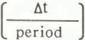(Δt being the sample interval, which in this case is one year) and denotes dimensionless frequency.

Figure 2(a) shows a plot of the spectrum of the noise model (thick curve). It appears that most of the spectral density or power is in the high frequency end of the spectrum. By analogy to light, such a spectrum could be termed “blue”. Similarly we shall regard the noise in annual layer thickness records as blue noise by analogy with the well-known concepts of white noise characterized by a uniform spectral density function and red noise characterized by concentration of the power in the low frequency end of the spectrum. Also shown in Figure 2(a) are estimated λ noise spectra (thin curves) from Dye 3 and Crête, Greenland. All estimated spectra show typically blue appearances.

Fig. 2

(a). Power spectra of noise model for annual layer thickness series: relative power as a function of dimensionless frequency f=Δt/period (Δt=1 a) Thick curve; theoretical spectrum. Thin curves: “observed” λ noise spectra for Crête and Dye 3. (b). Power spectra of noise model for annual δ values. Relative power as a function of dimensionless frequency f=Δt/period (Δt=1 a). Thick curves: theoretical spectra. Thin curves: “observed” δ noise spectra for Crête and Dye 3.

Examination of Table II shows that the actual estimates of the first (lag-one) autocorrelation r₁(λ) are not significantly different from that predicted except for Dye 2 and North Central. A characteristic of both locations is that the δ seasonals are not very distinct, though for different reasons. At Dye 2 the 5 seasonals are disturbed due to refreezing in the firn of large amounts of percolating meltwater. In the case of North Central the δ seasonals are gradually obliterated due to rapid diffusion in the firn and have in practice disappeared 20 m below the snow surface corresponding to an age of about 50 a. Both are poor sites for extracting good λ series from δ(¹⁸O) cycles.

The difficulty in interpreting the δ seasonals, and the consequent reduction of the accuracy in separating the individual years, will introduce an additional λ noise term which is less blue than the noise term discussed in this section and which consequently will tend to whiten the noise.

For stations such as Crête, which has virtually no melt and well-defined δ years, there is a good agreement between the model and “measured” values of the autocorrelation function for all lags.

Of some interest is the question of how the noise variance of the mean value of the accumulation of several years changes when the number of years increases. In the case of white noise in annual series with variance σ² it is well-known that the noise variance of the M a means will decrease as σ²/M. In the case of blue noise the variance will decrease even more rapidly with increasing M, the noise variance of the M a means being σ²/M², (Reference Reeh and FisherReeh and Fisher 1983). This result is not surprising in terms of accumulation rates on ice caps. If a given spot receives more than the average annual snow accumulation one year, then it is likely to receive less during the next year. One of the few things known for certain about the accumulation areas of large ice caps is that the surface looks the same from year to year.

4.2 Noise due to errors of separation between consecutive layers

In the δ(¹⁸O) dating technique the points of separation between annual layers are in most cases defined at the pronounced δ minima of the record, which reflect the culmination of the winter cold.

One source of error is related to the sampling frequency used when cutting the core for δ(¹⁸O) measurements. The sampling frequency for the cores used in this study ranges from 8 to 16 samples per calculated year and, thus, the position of the δ minimum is defined within one sample length only.

Another source of error is due to the mass exchange by diffusion, which occurs mainly in the porous snow and firn of the upper layers (Reference JohnsenJohnsen 1977). This process shifts the original position of the δ minima. Minima with small (large) separations approach (retreat from) one another.

A characteristic of both kinds of separation error is that if the thickness of one layer is underestimated , then the thickness of the succeeding layer will most likely be overestimated . Thus, the noise due to separation errors resembles that of the blue accumulation noise. If, however, the δ seasonals show large deviations from the ideal regular sine curve shape, e.g. very pronounced in the case of the δ records from Dye 2 and North Central, only separation points between, say, every third or fifth year may be well-defined. In such cases the intervening points of separation are chosen more or less by chance and a white noise component is introduced.

5.1 Theoretical noise model

The mean δ value of the snow at a particular time of year is taken as a constant over area and is only dependent on the time of year. It is denoted by D_i and

where for one year δ* is the true temporal mean value unweighted by accumulation, A is the amplitude of the δ cycle and Δ_i is the normalized deviation of D_i from δ* (see Fig.1). Since D_i is associated with the thickness of the snow layer 1_i, we have the areal average annual δ as the accumulation weighted mean

Similarly, the annual δ value measured from a single site or core is

The development of the δ noise theory follows much the same line as for the accumulation series. However, unlike accumulation stratigraphy, δ(¹⁸O) profiles, signal and noise are subject to vigorous smoothing by diffusion. Reference JohnsenJohnsen (1977) has provided a theory of diffusion of δ(¹⁸O) in the firn. He shows that diffusion is by vertical mixing of water vapour in the porous upper 15 to 20 m of firn, or, more strictly, in the layer down to the depth at which firn density reaches a value of 0.55 g cm⁻³ and air spaces between crystals lose contact with each other, preventing further mixing. The ratio R between the final (after diffusion) amplitude A₁ and the initial amplitude A of a δ cycle of wavelength λ is given as

where the diffusion length L_f for water vapour (and species transferred with it) is 7 to 8 cm of ice.

Equation (5.2) shows that diffusion reduces the amplitude, and thereby the variance, of any given δ cycle, and, furthermore, that the reduction is greater for the higher frequencies. Hence the overall effect of diffusion is to reduce the total variance and to transform the δ series spectrum towards redness by reducing the high frequency power.

The theoretical spectral distribution, autocovariance and autocorrelation functions for annually-averaged δ noise series are developed in Reference Reeh and FisherReeh and Fisher (1983). The noise model is entirely determined by its autocovariance function or equivalently by its variance σ_N ²(δ) = c_o(δ) and autocorrelation function

The autocovariance function is

t = 1, 2 ……a

where

and

It appears from Equation (5.3) that the autocovariance function depends on several parameters, viz, k, L_f/λ, and ρ₁(d), of which σ_d ² and ρ₁(d) in turn depend on A, σ_e/λ, k,

and Δ_i Δ_i-1(see Equations (5.4) and (5.5)).

5.2 Parameters influencing the δ-noise model

The parameters influencing the δ-noise model are of a different nature, some being related to snow deposition , some to the annual δ cycle (A, ΣΔ² _i, ΣΔ_iΔ_i-1) and some to the physical properties of the firn (L_f).

(i) Parameters related to snow deposition

According to C U Hammer (personal communication) the number of distinguishable layers k in an annual accumulation, as determined by electric conductivity measurements of Dye 3 and Crête ice cores, is of the order of magnitude of 20 to 25. The temporal mean value of the annual layer thickness λ has been determined with great accuracy for the various locations (Table II). The relative areal variabilityσ_e/λ was found to have a constant value of 0.13 for all the ice-cap sites considered.

(ii) Parameters related to the annual cycle

The amplitude A of the annual δ cycle can be estimated from measured δ profiles. However, due to the rapid diffusive smoothing of high frequency oscillations in the upper firn, only cycles of age less than 1 or 2 years relative to the surface can be trusted to yield A.

Figure 3 shows A from various Greenland sites and for the Devon Island ice cap plotted against latitude (upper line). The A value for a given latitude is obtained by averaging A for the uppermost year for sites within half a degree of the latitude. Since 43 different δ profiles taken at different times have been used to obtain the data points represented, some of the errors inherent in using only the uppermost years have been reduced. The least squares linear fit to the data gives

Fig. 3

Seasonal δ amplitude A for the uppermost layer of snow on ice-cap sites versus latitude, and A for coastal stations, lower points. Ice-cap stations within 1/2 degree of latitude are averaged together. The lines are least squares linear fits. GR: Grønnedal, TH; Thule, SC: Scoresbysund, NO: Nord, UM: Umanak.

where the slope determined has a standard error of ±0.06.

As a check on this slope the measured A values for precipitation at five coastal Greenland stations over six years have also been plotted in Figure 3. (IAEA 1969, 1970, 1971, 1973, 1975, 1979, Reference DansgaardDansgaard 1964). The slope of the A latitude relationship for coastal stations is almost the same as for the ice-cap sites, namely 0.25±0.03. That the coastal amplitudes are systematically lower is not surprising considering the moderating effect of the ocean.

It should be mentioned that the latitude amplitude relationship given by Equation (5.6) breaks down for latitudes greater than 80°N. Two high-latitude profiles examined Agassiz Ice Cap (80°40ˈN) on Ellesmere Island and Hans Tausen Ice Cap (81°30ˈN) in north Greenland) have A about half that expected from Equation (5.6). This could be a “real” effect in the δ seasonal variations or could be due to the special characteristics of these two ice caps.

If the annual δ cycle is assumed to be shaped as a sine curve, the terms

are functions of k only. Since both terms are controlled by the variance of the sine function for k→∞, they have a common limiting value of 0.5. Both terms are rather close to their limiting values of k ≥ 12. Other shape functions than the sine curve will provide different values of the two terms. For example, sawtooth and box-shape profiles give limiting values of 0.33 and 1.0 respectively. The 0.5 value is used for these terms in the following calculations.

(iii) Parameters related to the physical properties of the firn

As already mentioned, the diffusion length L_f has been taken to be 80 mm of ice after Reference JohnsenJohnsen (1977).

5.3 Comparison of observed δ noise with the theoretical noise model

For a sinusoidal Δ_i, the first autocorrelation coefficient ρ₁(δ) of annual noise and the dimensioniess δ noise variance depend on λ and k only. For ρ_i(δ), the dependence on k can even be neglected, since variations of k in the interval 12<k<32 will change the value of ρ₁(δ) by a few percent only. The curve in Figure 4(a) is based on a sine-shaped annual δ cycle and a value of k equal to 20. The shape of the curve points to diffusion as the process that largely determines the “colour” of the δ-noise. The smaller the λ value, the larger the ρ₁ value, i.e. the redder the noise.

Fig. 4

Comparison of observed δ noise characteristics with theoretical values (smooth curves). Error bars of observed values indicate 68% confidence limits (corresponding to one standard deviation in the case of a normal distribution).

(a) First serial correlation coefficient r₁(δ).

(b) Dimensionless 5 noise variance (σ_N(δ)·λ)²(σ_N(λ)A)² as functions of annual layer thickness. DE: Devon Island, CC: Camp Century, NC: North Central, CR: Crête, MC: Milcent, D2: Dye 2, and D3: Dye 3. For definition of other symbols see text.

The size of the dimensioniess noise variance is much more dependent on k than is ρ₁(δ), as illustrated in Figure 4(b). Also plotted in Figure 4(b) are the “measured” estimates of ρ₁, and i.e. r₁ and . In general, the “observed” values of r₁(δ) are in accordance with the theoretical, and the smaller the λ values are the larger are the r₁ values. However, for some locations (Dye 2 and Devon Island), the deviations of the “observed” values from the theoretical curve are significant at the 5% level. In the case of Dye 2, the low observed value is probably due to a reduced diffusion caused by the frequent occurrence of ice layers in the firn formed in connection with the percolation-refreezing process. The ability of ice layers to stop diffusion in the firn effectively has been demonstrated by the observation of extraordinarily large δ(¹⁸O) gradients associated with firn samples sandwiched between ice layers.

The high r₁ value for the Devon Island ice cap indicates that the L_f value used in the calculations is too small. This also seems to be the case for Camp Century. An increase of the diffusion length from 8 to 10 cm will bring the theoretical curve (thin curve in Figure 4(a)) into closer agreement with most of the observed values. The large uncertainty in the “observed” dimensionless variances (δ) (Fig,4(b)) precludes firm conclusions. However, the agreement between theory and observations is satisfactory. All (δ) values are close to 0.4. Using this value and the constant value of 0.017 found in section 3 for the relative λ noise variance, i.e. =0.017, gives

This expression points to the amplitude of the annual δ cycle as the main factor in determining the level of the δ noise. This is confirmed by the plot in Figure 5 showing the observed σ_N(δ) as a function of latitude.

Fig. 5

“Observed” δ noise standard deviations versus latitude of corresponding site of core recovery. Error bars indicate 68% confidence limits (corresponding to one standard deviation in the case of a normal distribution). Thick curve is the regression line. Thin curve is obtained from the noise model described in the text. DE: Devon Island, CC: Camp Century, NC: North Central, CR: Crête, MC: Milcent, D2: Dye 2, and D3: Dye 3.

σ_N(δ) shows a steady increase from south to north in accordance with the increase of the amplitude of the annual δ cycle (see Fig.5). The least squares linear fit to he data gives

where the slope determined has a standard error of 0.003. This regression line (thick line in Figure 5) does not deviate significantly from the line obtained by combining Equations (5.6) and (5.7) (thin line in Figure 5).

The theoretical power spectra for annually-averaged local δ noise is (Reference Reeh and FisherReeh and Fisher 1983)

In this equation PMA(f) is given by the expression

Figure 2(b) shows plots of theoretical (thick curves) and observed (thin curves) δ noise spectra for Crête and Dye 3. The agreement is satisfactory. The power is concentrated at the low frequencies and all the spectra can be termed red.

6.1 Comments on the noise models

The theoretical noise models presented should be considered first approximations only. Tacitly it has been assumed that the snow layers deposited by the individual storms are not mixed. In nature some mixing will always occur, the snow surface left by one storm being eroded by its successor. A comparison of the typical wave height of the winter snow-surface undulations of 0.26λ deduced in section 3 to the average thickness of the snow layer deposited by a single storm (0.05λ if k=20) clearly shows that mixing will occur, An approximate way of taking into account the mixing would be to apply a nominal k less than the actual one. However, the wide confidence limits of the “observed” model parameters do not allow any firm conclusions as to the magnitude of such a reduction. It is also worth remembering that in our model seasonal variations in roughness and shape changes from year to year have been neglected. Also in our development the ϵ_i terms, introduced in Equation (4.2), are assumed (for want of data) to be Gaussian, In fact, the ϵ_i terms with other stationary distributions would give similar theoretical noise models. The agreement we obtain between theoretical predictions and measurements suggests that either by chance the sastrugi are Gaussian or that the noise model is not very sensitive to the exact form of the ϵ_i distribution.

6.2 The signal-to-noise variance ratio

The signal-to-noise variance ratios F_λ and F_δ of the λ and δ series given in Table II show significantly higher values (2 to 3) for the southern and northern sites than for central sites (1 to 1.5). This is illustrated in Figures 6(a) and (b), where the thick line is a second degree curve fitted by least squares to the data. The second degree curve turns out to be the lowest degree polynomial, for which the sum of the squares of the deviations about the curve is not significantly larger than the expected value calculated by means of the standard deviations of the individual points.

Fig. 6

Signal-to-noise variance ratios F_λ and F_δ versus latitude of the site. Error bars indicate 68% confidence limits (corresponding to one standard deviation in the case of a normal distribution). Thick curves: second degree curve fitted to the data points by least squares. DE: Devon Island, CC: Camp Century, NC: North Central, CR: Crête, MC: Milcent, D2: Dye 2, and D3: Dye 3.

In the case of the λ series, the trend of the F_λ curve is due to a similar trend of the relative signal variances, the relative noise variance being independent of latitude (see Table II, column 3). This points to relatively stable precipitation conditions on a year-to-year basis in central Greenland, compared to more pronounced variations in north-west and south Greenland. In south Greenland variations are probably related to the proximity of strong westerlies and consequent variable weather conditions.

For δ series, the explanation of the trend of the F_δ curve is more complicated. In this case, records from southern and central sites have equal signal variances, whereas the signal variances of northern records show increased values. Combining this pattern with the steady south to north increase of the δ noise variance (Fig.5), leads to the appearance of Figure 6(b).

6.3 Delta records and diffusive smoothing

The large influence of the diffusive smoothing on the “colour” of the observed δ noise has already been pointed out. Obviously diffusion affects the signal part of a δ record in a similar manner. The redness of δ series spectra is partly a diffusion effect which is in turn sensitive to accumulation λ. Thus, before conclusions about the “colour” of climate-related variables are drawn from δ series, allowance should be made for diffusion and possible variations in diffusion related to changes in λ. It is important for interpreting spectral peaks of ice-core-derived time series to know the noise background spectrum and, for diffusing species, to realize that much of the reddening in the δ spectra could be due to diffusion effects.