

Introduction
The sustained interest in and fascination with carbon has been driven by the combination of its diversity, often extreme properties, and ultimately its current and future applications. Carbon’s four valence electrons ([He]2s 22p 2) can “blend,” or hybridize, giving it the ability to appear in many forms—the allotropes of carbon. From diamond, graphite, glassy, and hard carbons, to graphene, nanotubes, carbyne, and various forms of coal and soot, all are familiar faces of the ubiquitous carbon. Some carbon allotropes (diamond and graphite) have been known and used for centuries.
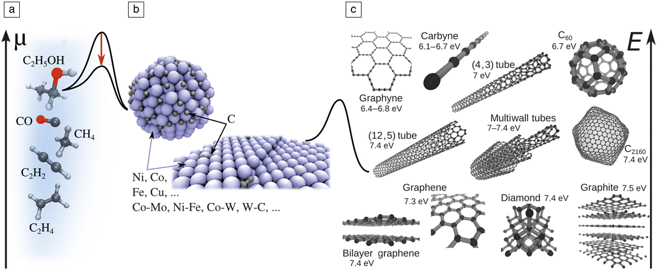
Yet, what nature offers (quality, quantity, and effective dimensionality) does not always allow for achieving the desired properties, leading to the need for carbon engineering. The first step involves the intentional, targeted synthesis of the desired material form—a rich and ever-expanding area of carbon research. Among the variety of synthetic methods, those that meet expectations for control and scalability are based on catalytic processing, where a carbon source (typically a hydrocarbon feedstock gas) is decomposed and the carbon atoms assemble in the new, desired pure-carbon form. The energy profile of such a process is quite complex, and understanding or predicting it is a long-standing challenge for theory ( Figure 1 ). The process involves a sequence of activated steps with high barriers, calling for the use of catalysts.
From common C sources to stunning nanoforms: (a) ethanol, carbon monoxide, methane, acetylene, and ethylene (C: black; H: white; O: red). Hydrocarbon decomposition quasi-equilibrium, C
x
H2y
↔ xC + yH2, would result in chemical potential
 $x\mu = \mu _{{C_x}{H_{2y}}}^0 - y\mu _{{{\rm H}_2}}^0 + {k_{\rm B}}T\,\ln \left( {{{{p_{{C_x}{H_{2y}}}}} / {p_{{H_2}}^y}}} \right)$
, with k
B, the Boltzmann constant; T, the temperature; “0,” indicating standard-state chemical potentials; and p
i
, the partial pressures. (b) Midsection shows a particle or substrate of the catalyst, and how it reduces the barriers (red downward arrow), at either stage of (left) feedstock cracking or (right) C insertion onto produced nanocarbon. (c) Representative family of carbon nanoforms and their cohesive energies E per C atom.
Except for very few cases, such as templated growth of CNTs, or multiwalled CNT growth in arc discharge, a catalyst is necessary for CNT growth. Experimentally, Fe, Co, Ni, or their alloys (e.g., Co-Mo, Reference Bachilo, Balzano, Herrera, Pompeo, Resasco and Weisman1 Ni-Fe Reference Chiang and Sankaran2 in chemical vapor deposition [CVD], Ni-Y in arc discharge) have been established as the best catalysts for CNTs. Although they have been widely used for more than a decade, there is still no generally accepted explanation for their efficiency. Recent observations further suggest that the alloy composition has an effect on chirality distribution. Reference Chiang and Sankaran2,Reference Chiang, Sakr, Gao and Sankaran3
The catalyst plays several important roles in the growth of nanocarbons: Reference Dupuis4,Reference Jourdain and Bichara5 (1) to decompose precursor molecules to release free carbon atoms or small clusters; (2) to serve as a solvent/carrier for these free carbon atoms; (3) to initiate CNT nucleation, when the C concentration on the catalyst is sufficiently high, via the sequence small carbon islands → graphitic caps → short CNTs → long CNTs; and (4) in steady-state growth, the catalyst successively decomposes the feedstock and transfers the released C by diffusion to the open tube edge.
The first two roles are common for the synthesis of nanocarbons. Crucially, for a broad class of other reactions of C x H y and CO on various metal surfaces, it is found through first-principles calculations Reference Bligaard, Nørskov, Dahl, Matthiesen, Christensen and Sehested6,Reference Abild-Pedersen, Greeley, Studt, Rossmeisl, Munter, Moses, Skúlason, Bligaard and Nørskov7 that transition-state energies to adsorption (E ‡) and the dissociative chemisorption energies (∆E) follow a Brønsted–Evans–Polanyi type linear relation, Reference Bligaard, Nørskov, Dahl, Matthiesen, Christensen and Sehested6 E ‡ ∼ ∆E. For the overall reaction rate K in the case of the rate-limiting dissociative adsorption of a C x H y precursor, one has Reference Nørskov, Bligaard, Logadottir, Bahn, Hansen, Bollinger, Bengaard, Hammer, Sljivancanin, Mavrikakis, Xu, Dahl and Jacobsen8,Reference Robertson9 K ∼ ε/(const + ε) Reference Chiang and Sankaran2 , with ε ≡ exp(–∆E/k B T), where k B is the Boltzmann constant and T is the temperature. In both limiting cases of large ε and small ε, K → 0, resulting in the so-called Sabatier volcano-plot Reference Bligaard, Nørskov, Dahl, Matthiesen, Christensen and Sehested6,Reference Robertson9 with a pronounced maximum in an intermediate, optimal range of ∆E. The critical finding that allows for the rational search for and optimization of the catalyst is that ∆E correlates with the position of the d-band center relative to the Fermi energy in transition metals—a “descriptor” of catalytic activity accessible from accurate but feasible electronic structure calculations.
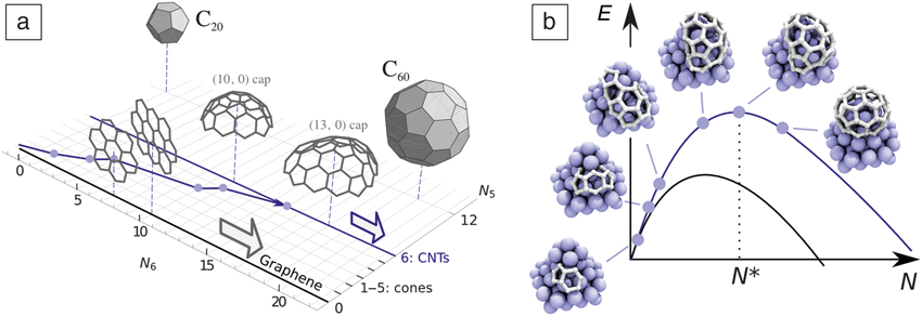
CNTs and graphene differ considerably during the nucleation stage. The honeycomb lattice tessellates the plane. After a stable planar nucleus is formed, graphene can grow by adding only new hexagons. A CNT is a cylinder, which means that an initial carbon nucleus is topologically required to exactly incorporate six pentagons. A map of carbon nanoforms and their transformations using the number of hexagons N 6 and pentagons N 5 as coordinates is quite instructive (see Figure 2a). Reference Penev, Artyukhov and Yakobson10 Graphene islands/flakes of any size are represented by the N 5 = 0 line, with N 6 → ∞ being the ideal infinite honeycomb lattice. One to five pentagons represent the small family of carbon nanocones whose angle at the tip has discrete values, depending on N 5.
(a) Carbon forms projected onto the number of hexagons (N 6) and pentagons (N 5) coordinate plane. Reference Penev, Artyukhov and Yakobson10 The blue line illustrates a gradual formation of a carbon nanotube (CNT) cap, with points indicating incorporation of a new pentagon. (b) Schematic energy (E) profiles as a function of system size N for CNTs (blue curve; N* is the critical nucleus size) and graphene (black curve). Images show a CNT cap nucleus on a Ni cluster as it incorporates the six required pentagons, Reference Luo, Penev, Harutyunyan and Yakobson13 along the blue path shown in (a).
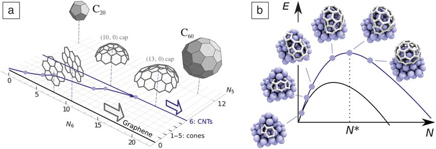
Once the N 5 = 6 line is reached, the corresponding hemispherical cap is suitable to evolve into a cylinder, or liftoff the catalyst surface, Reference Pigos, Penev, Ribas, Sharma, Yakobson and Harutyunyan11 unlike the graphene that always remains grounded. From the point of view of classical nucleation theory Reference Kuznetsov, Usoltseva, Chuvilin, Obraztsova and Bonard12 (Figure 2b), the trajectory in the (N 6, N 5) plane, leading to the N 5 = 6 line, increases in energy to reach the critical nucleus cap of N* carbon atoms. The cylindrical topology of a CNT entails another, crucial, difference from graphene: nanotubes can be helical, or chiral, as they can be obtained by rolling up a graphene strip in many possible ways to form a cylinder. This is specified by the chiral vector C = n a 1 + m a 2, where a 1,2 are the honeycomb lattice vectors, and the pair of non-negative integer components (n, m) are referred to as chiral indices.
Such distinction leads to different goals and challenges in the experimental synthesis of carbon nanoforms. Graphene needs to be grown rapidly and achieve large-area, high-quality monocrystals or bilayers, while long CNTs of controlled type (n, m), are the target. Theoretical models and simulations Reference Elliott, Shibuta, Amara, Bichara and Neyts14,Reference Amara and Bichara15 are indispensable in achieving these goals, and we next briefly discuss the scope of the methodologies used, and then, in more detail, the separate specifics for graphene and CNTs.
Modeling approaches in a nutshell
The importance of a wide range of length- and time scales is generic in the synthesis of complex materials such as nanocarbons. The theoretical description of such systems requires more than a single theoretical tool, entailing more diverse methodological, software, and hardware requirements. Typically, a suitable set of methods and tools can be used to study a broader spectrum of physical/chemical properties and processes related to the catalytic CVD growth of graphene, CNTs, and other carbon nanoforms. Such a methodological toolkit generally includes structure identification through ground-state total energy minimization, or molecular dynamics (MD) Reference Frenkel and Smit16 mimicking the actual thermal motion and time evolution at finite temperatures.
The stochastic nature of crucial processes such as atomic rearrangements during nucleation and growth can be represented by Monte Carlo (MC) methods. Reference Landau and Binder17 The underlying interatomic interactions (energies, forces) are described at different levels of theory, with the particular choice dictated by the system size and time scale of interest—from classical empirical potentials, constructed and parameterized for a specific set of species, and the tight-binding approximation Reference Goringe, Bowler and Hernández18 based on predesigned wave functions and their overlaps, to the first-principles density functional theory (DFT). Reference Dreizler and Gross19 The last (and eventually DFT-based tight-binding) level of description has the advantage of accuracy in energy or reaction-barrier evaluations, but may become computationally expensive for MD simulations (accessible time scale in DFT-based MD simulations is generally a few ps for a system of approximately 100 atoms, and ∼10 ps in tight-binding based MD simulations of similar size systems).
An attempt to circumvent the time scale problem in CNT modeling, for example, is based upon a hybrid approach in which an intermittent classical MD growth trajectory is initiated, interrupted regularly by MC relaxation cycles, producing single-wall CNT with “definable,” Reference Neyts, Shibuta, van Duin and Bogaerts20 yet occasionally changing chirality, but offers no rigorous connection with physical time. This would be, in principle, possible through kinetic MC schemes that can tackle the CVD Reference Battaile and Srolovitz21 growth process and were used to address some aspects of graphene Reference Zangwill and Vvedensky22 and CNTs Reference Grujicic, Cao and Gersten23 synthesis.
In the efforts toward more realistic modeling, especially of the initial stages of CNT growth, the chemical state (e.g., pure metal, oxide, surface, or bulk carbide) of the catalyst is of particular importance. Grand-canonical MC simulations have provided a more detailed picture of the C-precursor adsorption thermodynamics, defects healing, as well as the correlation between the CNT diameter and size of the catalyst particle. Reference Amara, Bichara and Ducastelle24–Reference Magnin, Zappelli, Amara, Ducastelle and Bichara26
Theory and simulation of graphene CVD catalytic growth
On a spatially expansive planar catalyst, carbon atoms typically assemble into a single layer, graphene, in a way similar to the addition of an adlayer in normal 3D crystal growth. One can distinguish three stages in growing a full graphene layer on a catalyst surface as (1) the nucleation of graphene; (2) the lateral expansion growth of the graphene islands; and (3) the coalescence of numerous graphene islands into a complete graphene sheet, either with the formation of grain boundaries or—often desirably—without seams. As a heteroepitaxial process, graphene growth on a catalyst surface is also very different from the formation of an adlayer during 3D crystal growth. Graphene is highly flexible and interacts only weakly with most substrates, and therefore, its growth behavior is also different from the well-explored heteroepitaxial growth of thin films.
In stage (1), the barrier to graphene nucleation, concentration, and diffusivity of the carbon precursor (e.g., atomic C, dimer C2, or radicals CH and CH2) on the substrate are the critical factors that determine the rate of nucleation and the density of the nuclei. Since all three key factors depend on the catalyst surface, the nucleation of graphene must also be substrate dependent. Theoretical studies have revealed that due to the large formation energy of the graphene edge bent toward the catalyst surface, the nucleation barrier of graphene on a metal surface can be as high as 8.0 eV, and the rate of nucleation can be as low as 10–6 cm–2s–1. Reference Gao, Yip, Zhao, Yakobson and Ding27 This means that graphene nucleation can be suppressed or avoided by planting seeds on a catalyst surface, and it is possible to achieve a low nucleation density by using a low feedstock concentration. Painstakingly in experiments, lowering the density of the nuclei down to ∼0.1 to 1 per mm2 has been achieved, Reference Hao, Bharathi, Wang, Liu, Chen, Nie, Wang, Chou, Tan, Fallahazad, Ramanarayan, Magnuson, Tutuc, Yakobson, McCarty, Zhang, Kim, Hone, Colombo and Ruoff28–Reference Chen, Zhao, Xiang, Kim, Cha, Chiashi and Maruyama31 and an ultralow density of 10–3 to 10–4 per mm2 was achieved by the local precursor feeding technique, for the growth of a wafer-size single crystal. Reference Wu, Zhang, Yuan, Xue, Lu, Liu, Wang, Wang, Ding, Yu, Xie and Jiang32
As in any heteroepitaxial process, graphene nucleation sensitivity to the catalyst surface is quite significant. On Ru(0001) and Ir(111) surfaces, all the precursors form stable carbon clusters (combination of hexagons and pentagons), C21 or C24. Reference Wang, Ma, Caffio, Schaub and Li33,Reference Yuan, Gao, Shu, Zhao, Chen and Ding34 These clusters are exceptionally stable and are considered as intermediate structures, a “stopping point” between a carbon precursor and the graphene island. Therefore, the nucleation density is normally very high due to the low diffusivity of these highly stable intermediates. Reference Yuan, Gao, Shu, Zhao, Chen and Ding34
The lateral graphene growth, stage 2, at the atomic level is a consequence of net carbon accretion to the graphene edge. Considering the reverse action, the growth rate at a graphene edge can be written as R ∼ R att – R det, where R att = c R 0 exp(–E*/k B T), with R 0 ≡ k B T/h and h being Planck’s constant, is proportional to the flux of carbon atoms attachment from the catalyst surface, where c is the concentration of C atoms on the surface and E* is the barrier of C-attachment; R det = R 0 exp[–(E*+E R)/k B T], where E R is the reaction energy of the carbon attachment. The rate of graphene growth is R = R 0 exp(–E*/k B T) [c – exp(–E R/k B T)], and thermal equilibrium can be reached at concentration c eq ∼ exp(–E R/k B T). Since E R is the formation energy of the carbon precursor on the catalyst surface, its concentration during graphene growth strongly depends on the activity of the metal.
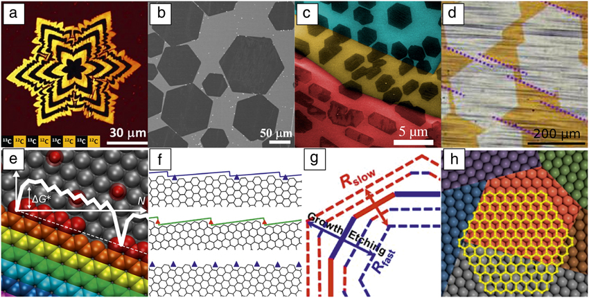
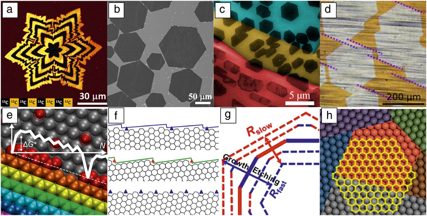
From previous studies, one can classify the catalysts into two categories: Reference Wang, Yuan, Li and Ding35 a relatively inert catalyst surface (e.g., Cu and Au) where the C-precursor has a formation energy >2.0 eV, and the active catalysts (e.g., Pd, Pt, Ni, Ru, Rh, It) with formation energy of the carbon precursors around 1.0 eV or less. For the case of graphene growth on a Cu or Au surface, the low concentration of the precursor (coverage down to 10–8) and the low activity of the catalyst require the long-distance diffusion of carbon precursors to feed the graphene growth. Therefore, the behavior of graphene growth is often diffusion-limited as evidenced by the star- or fractal-like dendritic flakes commonly observed. Reference Hao, Bharathi, Wang, Liu, Chen, Nie, Wang, Chou, Tan, Fallahazad, Ramanarayan, Magnuson, Tutuc, Yakobson, McCarty, Zhang, Kim, Hone, Colombo and Ruoff28,Reference Wang, Yuan, Li and Ding35,Reference Xu, Zhang, Qiu, Zhuang, Zhang, Wang, Liao, Song, Qiao, Gao, Hu, Liao, Liao, Yu, Wang, Ding, Peng and Liu36 Different from Cu and Au, the carbon precursor concentration on active catalyst surfaces is orders of magnitude higher, and the active surface can ensure sufficient precursor flux across the catalyst. This maintains the edge-kinetics-limited (as opposed to diffusion-controlled) growth of graphene. In this regime, graphene islands display regular shapes, determined by the kinetic Wulff construction, as is broadly observed Reference Gao, Ren, Xu, Jin, Wang, Ma, Ma, Zhang, Fu, Peng, Bao and Cheng37 ( Figure 3 ). Reference Hao, Bharathi, Wang, Liu, Chen, Nie, Wang, Chou, Tan, Fallahazad, Ramanarayan, Magnuson, Tutuc, Yakobson, McCarty, Zhang, Kim, Hone, Colombo and Ruoff28,Reference Geng, Wu, Guo, Huang, Xue, Chen, Yu, Jiang, Hu and Liu38–Reference Zhang, Xu, Hui, Xin and Ding43 This concept is an analogue to the equilibrium Wulff shape, but is based on the anisotropic growth rate Reference Sekerka44 (see Figure 3g).
Experimental graphene domains. (a) Raman map of star-like graphene domains marked by using carbon isotopes. Reference Hao, Bharathi, Wang, Liu, Chen, Nie, Wang, Chou, Tan, Fallahazad, Ramanarayan, Magnuson, Tutuc, Yakobson, McCarty, Zhang, Kim, Hone, Colombo and Ruoff28 (b) Scanning electron microscope (SEM) image of hexagonal graphene domains grown on a liquid-copper surface. Reference Geng, Wu, Guo, Huang, Xue, Chen, Yu, Jiang, Hu and Liu38 (c) SEM image of graphene domains on a polycrystalline Cu foil (Cu grains are highlighted in different colors); the shapes are modulated by the interaction between graphene and the substrate. Reference Artyukhov, Hao, Ruoff and Yakobson39 (d) Optical image of coalescence of unidirectionally aligned graphene domains on the Cu(111) surface. Reference Xu, Zhang, Dong, Yi, Niu, Wu, Lin, Yin, Li, Zhou, Wang, Sun, Duan, Gao, Jiang, Wu, Peng, Ruoff, Liu, Yu, Wang, Ding and Liu40 Edges of the domains marked by dotted lines are parallel to each other. (e–h) Modeling of shapes and growth rates of graphene. Reference Artyukhov, Liu and Yakobson41–Reference Zhang, Xu, Hui, Xin and Ding43 (e) The growth of the symmetric edges. Reference Artyukhov, Liu and Yakobson41 Each successive row of carbon atoms is shown in a different color. The graph illustrates the free energy of the system G as a function of size N with the characteristic nucleation barrier ΔG*. The dashed line indicates the overall trend of linear energy decrease, −NΔµ, with increasing system size (N), and slope determined by the chemical potential (µ) of the carbon source. (f) Tilted edges, viewed as (top) armchair or (middle) zigzag edges with series of kinks (triangles). The bottom image shows the edge with 19.1° tilt angle. (g) Applying the kinetic Wulff construction Reference Artyukhov, Liu and Yakobson41,Reference Ma, Ren, Zhang, Liu, Gao, Yin, Ma, Ding and Cheng42 during growth (outward arrow) and etching (inward arrow), red and blue edges representing slower and faster growth/etching, with rates R slow and R fast, respectively. (h) A graphene domain (yellow) crosses a grain boundary of the catalyst surface without changing orientation. Reference Zhang, Xu, Hui, Xin and Ding43
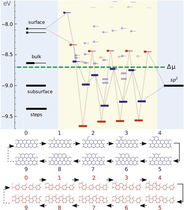
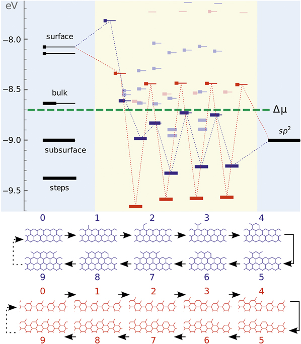
As an elementary step of graphene growth, carbon addition can be described by the previously mentioned equations. But during the overall graphene island growth process, the barriers and the reaction energies of adding a C atom are highly dependent on the local environment, especially the atomistic details of the edge itself. As shown in the nanoreactor diagram in Figure 4 , a carbon atom can be added to many possible sites, and the addition of C to an armchair (AC) site is different from that to a zigzag (ZZ) edge and sensitively depends on the order of addition. Reference Artyukhov, Hao, Ruoff and Yakobson39,Reference Ma, Ren, Zhang, Liu, Gao, Yin, Ma, Ding and Cheng42 Because this is rather heterogeneous, varying from site to site, graphene growth is far more complicated than an elementary chemical reaction.
Nanoreactor diagram for zigzag- (blue) and armchair-type (red) edges grown on a Ni substrate. Carbon atoms migrate from the source (metal substrate, leftmost levels) to the sp Reference Chiang and Sankaran2 product (graphene, rightmost) by sequentially populating intermediate states in the middle. The state occupancies at k B T = 0.1 eV are represented as thicker segments. Lowest-energy atomic configurations (corresponding to the levels connected by dotted lines) upon sequential addition of 0 to 9 carbon atoms (labels above each image) are shown at the bottom. The feedstock gas, Figure 1a, sets the chemical potential μ of carbon atoms (green dashed line). Reference Artyukhov, Liu and Yakobson41
From the point of view of crystal growth, the formation of every row of carbon atoms along a highly symmetric edge (AC or ZZ) has two elementary steps—the nucleation of a 1D seed, which in general just requires forming a single hexagon by inserting 2–3 atoms onto the edge, and then fast propagation of kinks in both directions from such a nucleus, with every repeatable step adding two atoms. Calculations have clearly demonstrated that on most catalyst surfaces, the larger kinks on a ZZ edge have a higher energy of nucleation than on an AC edge, and, therefore, the growth rate of a ZZ edge is lower than that of an AC edge. In comparison with these two highly symmetric edges, all other edges could be seen as high-symmetry ones but with kinks, and therefore, growing faster. Among them, the one with a 19.1° tilt angle (from the ZZ direction) has the maximum number of kinks. In general, the growth rate of graphene edges on a catalyst surface follows the sequence Reference Ma, Ren, Zhang, Liu, Gao, Yin, Ma, Ding and Cheng42,Reference Rao, Liptak, Cherukuri, Yakobson and Maruyama45 of R ZZ < R AC < R tilt < R 19°, where R tilt is the growth rate of an edge with an intermediate tilt angle.
By applying this result to the kinetic Wulff construction, one can easily explain why most observed graphene edges are ZZ type. Even though reduced symmetry of the substrate, including the presence of metal steps or kinks, may modulate the growth rates at graphene edges, the ZZ type is still the most observed. Reference Artyukhov, Liu and Yakobson41 As an example, the shape of a graphene domain at a steady state of either growth (ZZ hexagon) or etching (19°-edged dodecagon) could be well explained by applying kinetic Wulff-construction analysis. Reference Ma, Ren, Zhang, Liu, Gao, Yin, Ma, Ding and Cheng42
For high-quality graphene, the growth of large single crystalline domains is essential. Theoretically, there are two possible routes: (1) gradual development of a single seed over the area of the catalyst substrate; and (2) the seamless coalescence of multiple, but unidirectionally aligned, islands into a single crystal. Route 1 requires the CVD growth to not be strictly epitaxial, to allow single-crystal graphene to pass over the grain boundaries of the substrate without altering its single-crystal nature, while route 2 requires the unidirectional alignment of all the fusing domains. Calculations of the interaction between graphene and the catalyst surface show that the binding between the graphene and metal surface is weak and only slightly depends on the relative orientation angle between graphene and the substrate, Reference Zhang, Xu, Hui, Xin and Ding43 which supports the feasibility of route 1. Further calculations prove that a ZZ edge tends to be along [110] or equivalent direction on the catalyst surface Reference Nguyen, Shin, Duong, Kim, Perello, Lim, Yuan, Ding, Jeong, Shin, Lee, Chae, Vu, Lee and Lee46–Reference Yuan, Song, Sun and Ding48 due to better lattice matching, and therefore the perfect alignment of multiple domains on a single crystal catalyst can be maintained. Recently, the synthesis of inch-sized single-crystal graphene was achieved by route 1 Reference Wu, Zhang, Yuan, Xue, Lu, Liu, Wang, Wang, Ding, Yu, Xie and Jiang32 and the growth of meter-sized single crystal graphene has been realized using route 2. Reference Xu, Zhang, Dong, Yi, Niu, Wu, Lin, Yin, Li, Zhou, Wang, Sun, Duan, Gao, Jiang, Wu, Peng, Ruoff, Liu, Yu, Wang, Ding and Liu40
Another important factor in graphene growth is its rate, which is controlled by the carbon addition to an edge. A lower barrier to attachment leads to faster growth. Cu is a perfect catalyst because the large exothermicity of the precursor transfer from copper to graphene should result in a rather small barrier to this attachment event. Since Cu itself is not an active catalyst for most feedstock decompositions, a cocatalyst, such as a Ni-Cu alloy, or a continuous oxygen supply, is required to promote the growth of graphene on Cu as shown recently. Reference Hao, Bharathi, Wang, Liu, Chen, Nie, Wang, Chou, Tan, Fallahazad, Ramanarayan, Magnuson, Tutuc, Yakobson, McCarty, Zhang, Kim, Hone, Colombo and Ruoff28,Reference Wu, Zhang, Yuan, Xue, Lu, Liu, Wang, Wang, Ding, Yu, Xie and Jiang32,Reference Xu, Zhang, Qiu, Zhuang, Zhang, Wang, Liao, Song, Qiao, Gao, Hu, Liao, Liao, Yu, Wang, Ding, Peng and Liu36
Once two graphene islands meet, they should coalesce. The process of coalescence is critical for understanding the final stage of graphene growth—stitching numerous domains into a continuous film covering the entire catalyst surface. Depending on the type of edges and the angle of misalignment, there are two modes of stitching two domains together, either to form a grain boundary composed of a series of pentagon–heptagon 5|7-pairs, or to form a weakly bonded overlapping interface of the two domains. Theoretical analysis shows that the former could likely occur if graphene edges are metal-surface passivated, while the latter is preferred if both edges are hydrogen passivated. Reference Dong, Wang, Peng, Liu, Zhang and Ding49 A special case of full coalescence of graphene islands is their seamless stitching, requiring both domains to be unidirectionally aligned and covalent C–C bonds to form readily between the domains, which is far from trivial.
Carbon nanotubes
CNTs are now routinely grown using catalytic CVD. Comprehensive surveys of recent experimental and theoretical studies (ca. 2005–present) are available. Reference MacKenzie, Dunens and Harris50 The precursor gases (Figure 1) are as diverse as CO (high- or ambient pressure), methane (CH4), acetylene (C2H2, diluted or undiluted), or alcohols (methanol and ethanol). Cobalt dominates the catalyst elements (alloyed with Mo, W, or in pure form), but Fe is also well represented (pure or alloyed with Ni, Cu, or Ru). Both silica- and magnesia-supported catalysts are used, and in the case of Fe, unsupported floating-catalyst aerosol growth has been demonstrated. Finally, growth temperatures vary from ∼1000°C to as low as ∼500°C, with the lower temperatures initially showing perhaps the best selectivity, but recently, almost monochiral samples were achieved at the high-temperature end. Reference Yang, Wang, Zhang, Yang, Luo, Xu, Wei, Wang, Xu, Peng, Li, Li, Li, Li, Bai, Ding and Li51,Reference Zhang, Kang, Wang, Tong, Yang, Wang, Qi, Deng, Li, Bai, Ding and Zhang52
In spite of numerous experimental studies of the CNT growth mechanism, it has been hard to obtain the details beyond the phenomenological vapor–liquid–solid or vapor–solid–solid models through experiments only, because growth is sensitive to conditions (e.g., carrier gas, carbon feedstock, catalyst, temperature T, and substrate used) and in situ observations are difficult. In contrast, in theoretical model simulations, the growth parameters and position of each atom are well defined, which makes it possible to clearly discriminate between the critical factors. Early atomistic models, dating back to the mid- and late-1990s, focused on the growth process represented as C-atom addition to the open end of a freestanding CNT, without or with one or few catalyst atoms. Reference Maiti, Brabec, Roland and Bernholc53–Reference Buongiorno Nardelli, Brabec, Maiti, Roland and Bernholc55 While providing important insights, most of those simulations yielded fast end closure, and thereby growth termination, even with a few catalyst atoms. These studies revealed the importance of catalyst size.
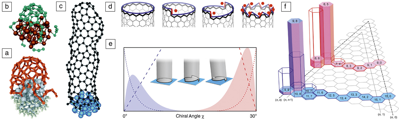
Although structure quality of the CNT suggests relatively organized assembly of C atoms on a catalyst, actual MD simulations have rarely produced nondefective structures or even a well-defined diameter and recognizable chirality. This is the case regardless of the level of interatomic potentials, from classical Reference Shibuta and Maruyama56–Reference Ribas, Ding, Balbuena and Yakobson59 to tight-binding Reference Zheng, Irle and Morokuma60,Reference Irle, Ohta, Okamoto, Page, Wang and Morokuma61 and DFT, Reference Raty, Gygi and Galli62 and is mainly caused by the MD time scale, inevitably limited to short intervals in which the atoms are forced to rapidly assemble without sufficient relaxation, due to sheer computational limitations. Yet, MD simulations have been instrumental in providing a demonstration of the liftoff process ( Figure 5a–c). Reference Raty, Gygi and Galli62–Reference Xu, Yan and Ding64
The early stages of carbon nanotube (CNT) growth—nucleation via liftoff captured at various levels of theory. (a) Density functional theory (DFT), Reference Raty, Gygi and Galli62 (b) DFT-based tight-binding, Reference Ohta, Okamoto, Page, Irle and Morokuma63 and (c) empirical force fields; metal atoms are shown in gray, brown, or blue spheres, respectively, and carbon as red, green, or black spheres, respectively. Reference Xu, Yan and Ding64 (d) The edge of a CNT viewed as a set of “cozy corners” (•) for C attachment, from (left) none for zigzag, to (middle) some intermediate values, to (right) a maximum for armchair. Reference Ding, Harutyunyan and Yakobson67 Black line highlights the CNT edge; blue and red lines represent the edge as a continuum of “smooth” ZZ segments and kinks, respectively. (e–f) The (e) abundance distributions A(χ) ∼ χ e –χ computed as the product of nucleation (dotted) and growth rate (dashed) terms, resulting in sharply peaked behavior near zigzag (blue), or near armchair chiralities (red); (f) two particular realizations for different CNT diameters are shown for solid (opaque bars), and liquid catalyst (empty bars); (n, m) are the chiral indices. The inset in (e) illustrates (left) achiral, (middle) multiple-kink chiral, and (right) single-kink chiral CNTs on a flat substrate. Reference Artyukhov, Penev and Yakobson75
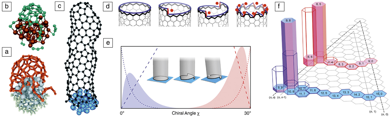
The time scale limitations in atomistic simulations have been circumvented in an analytical theory derived from crystal growth fundamentals. As early as the seminal paper by Iijima, Reference Iijima65 the connection between the structure of chiral CNTs and screw dislocations in crystals has been recognized. Screw dislocations are key for crystal growth under low supersaturations. Reference Burton, Cabrera and Frank66 This connection between the chirality of nanotubes and their growth was quantitatively established in 2009, relating the nanotube growth rate R with the chiral angle χ explicitly, Reference Ding, Harutyunyan and Yakobson67 R(χ) ∼ sin χ ≈ χ (Figure 5d). This equation predicts that AC nanotubes are the fastest growing, and the growth velocity decreases linearly from AC to ZZ nanotubes, for which the growth velocity becomes negligible due to the large energy barrier for the nucleation of each sequential ring of C atoms. The dislocation theory of nanotube growth was supported by the correlation between CNT abundance and χ in a number of independent experiments, Reference Ding, Harutyunyan and Yakobson67 further supported by in situ single-molecule experiments using field-emission projection imaging, Reference Marchand, Journet, Guillot, Benoit, Yakobson and Purcell68 and confirmed by Raman spectroscopy growth monitoring. Reference Rao, Liptak, Cherukuri, Yakobson and Maruyama45 Additional experimental backing comes from measurements on chirality-selected “cloned” CNTs. Reference Liu, Wang, Tu, Liu, Chen, Zheng and Zhou69 Recent MD simulations also show a greater growth velocity for large-χ (AC and near AC) nanotubes. Reference Li, Page, Irle and Morokuma70 The original derivation R(χ) ∼ sin(χ) ∼ χ relied on the observation (through DFT computations) of the absence of a nucleation barrier on AC edges; Reference Ding, Harutyunyan and Yakobson67 the underlying assumption being that the metal is compliant and rearranges to always follow the profile of the nanotube edge.
It may appear surprising and even counterintuitive that the dislocation theory prediction ∼ sin χ correlated well with the observed abundance of nanotubes in growth experiments, where multiple chiralities were detected simultaneously. Reference Ding, Harutyunyan and Yakobson67 The ∼ sin χ equation does not contain a nucleation term, whereas the measured abundance must be due to both the growth rate and nucleation probability. The observed good correlation then implies that the nucleation probability in the experiments analyzed in Reference Reference Ding, Harutyunyan and Yakobson67 is flat (i.e., independent of χ).
Over the last decade, multiple experiments have revealed a predominance of (n, n–1) types Reference Bachilo, Balzano, Herrera, Pompeo, Resasco and Weisman1,Reference He, Jiang, Liu, Fedotov, Chernov, Obraztsova, Cavalca, Wagner, Hansen, Anoshkin, Obraztsova, Belkin, Sairanen, Nasibulin, Lehtonen and Kauppinen71,Reference Wang, Wei, Ren, Wang, Pfefferle, Haller and Chen72 and several studies in 2013 reported such CNT types. This perceived mystery Reference He, Jiang, Liu, Fedotov, Chernov, Obraztsova, Cavalca, Wagner, Hansen, Anoshkin, Obraztsova, Belkin, Sairanen, Nasibulin, Lehtonen and Kauppinen71 of the essentially complete absence of pure-AC nanotubes and of the profound nonlinearity of the abundance A(χ) points to the need for a unified approach to CNT chirality that reconciles the thermodynamics Reference Liu, Dobrinsky and Yakobson73 and kinetics arguments previously mentioned. Reference Marchand, Journet, Guillot, Benoit, Yakobson and Purcell68 Minimally chiral tubes (i.e., closest to the achiral AC and ZZ types, (n, n–1) or (n, 1), respectively) can be understood as a result of two opposing trends at the nanotube–catalyst interface—an energetics preference for achiral tubes (lack of kinks and tight contact) versus faster growth rate for chiral tubes (more loose contact, with kinks). This concept is quite generic and such behavior can be shown to emerge even for a continuum representation of the interface between a CNT and a solid catalyst (Figure 5e), or within jellium model. Reference Artyukhov, Liu, Penev and Yakobson74
A crucial aspect in this approach Reference Artyukhov, Penev and Yakobson75 is the explicit representation of the CNT-type abundance as a product of a nucleation probability N(χ) and a growth-rate term R(χ): A(χ) = N(χ) • R(χ). Atomistic simulations show that on a solid particle, the interplay between interface energetics (N ∼ e –χ) and kinetics (R ∼ χ) leads to a sharply peaked distribution (Figure 5e–f). On the other hand, nucleation is only weakly χ-sensitive on fully compliant liquid catalysts, leading to a broader A(χ) distribution, generally increasing toward AC types. Such “kinetic route” of chiral selectivity, governed by R(χ), may preferentially produce (2m, m) tubes, corresponding to χ = 19.1° where the number of kinks reaches a maximum equal to m, and these tubes are the fastest growing. Interestingly, the recent high purity (12, 6)-tubes, obtained using Co7W6 Reference Yang, Wang, Zhang, Yang, Luo, Xu, Wei, Wang, Xu, Peng, Li, Li, Li, Li, Bai, Ding and Li51 or Mo2C catalysts, Reference Zhang, Kang, Wang, Tong, Yang, Wang, Qi, Deng, Li, Bai, Ding and Zhang52 and (8, 4)-tubes, using a WC catalyst, Reference Zhang, Kang, Wang, Tong, Yang, Wang, Qi, Deng, Li, Bai, Ding and Zhang52 both belong to the same (2m, m) type. Although these studies emphasize the “epitaxial” matching (implying low-energy interfaces) between the tubes and specific crystal planes of the solid catalysts, the jury is still out on the true origin of such exceptional preference.
A distinctly different approach toward chirality specific CNT synthesis is to entirely circumvent the inherently stochastic nucleation stage. In a recent experiment, Reference Sanchez-Valencia, Dienel, Gröning, Shorubalko, Mueller, Jansen, Amsharov, Ruffieux and Fasel76 truly single-chirality, AC (6, 6) CNTs were produced using growth from rationally designed molecule seeds. Reference Scott, Jackson, Zhang, Steinberg, Bancu and Li77 The CNT material yield, however, was low and calls for a better understanding of the growth kinetics of achiral tubes in general. From a modeling perspective, this work also provokes the question of designed precursors that would allow for chiral seeds, and hence, single-type chiral CNTs.
Summary
Catalytic CVD has been one of the most promising routes toward the scalable and controllable synthesis of a plethora of carbon nanoforms. At the same time, it poses a daunting challenge associated with exploring and finding optimal domain(s) in the inherent vast parameter space (sources, choice of catalysts, and growth conditions). Theoretical models and a broad spectrum of simulation techniques have turned into an indispensable toolkit complementing experimental efforts and often providing unique guidelines and predictions. In conjunction with automated or even autonomous experimentation, Reference Nikolaev, Hooper, Perea-López, Terrones and Maruyama78 such models are crucial in advancing multiple new carbon nanomaterials to the “slope of enlightenment.” Reference Davenport79 Systematic efforts in catalyst engineering Reference Xu, Kaneko, Shibuta and Kato80 ensure the sustained progress toward desired practical applications.
Acknowledgments
E.S.P. and B.I.Y. acknowledge support from the National Science Foundation (CBET 1605848), the Air Force Office of Scientific Research (FA9550-14–1-0107), and the Office of Naval Research (N00014-15-1-2251). F.D. acknowledges support from the Institute of Basic Science, South Korea.
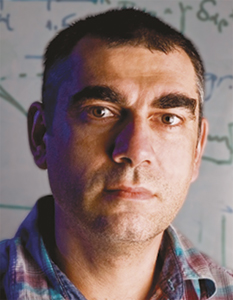
Evgeni S. Penev is an assistant research professor at Rice University. He studied physics at the St. Clement of Ohrid University of Sofia, Bulgaria, and received his MS degree in solid-state physics. He received his PhD degree from the Fritz Haber Institute of the Max Planck Society, Germany, and was awarded the Otto Hahn Medal for outstanding scientific achievement. Penev can be reached by phone at 713-348-5979 or by email at epenev@rice.edu.
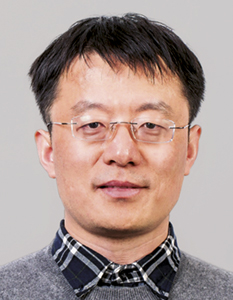
Feng Ding is a distinguished professor at the Ulsan National Institute of Science and Technology and a group leader in the Center for Multidimensional Carbon Materials, Institute for Basic Science, South Korea. He received his PhD degree from Nanjing University, China, in 2002. He worked at the University of Gothenburg, Sweden, Rice University, and The Hong Kong Polytechnic University as a research scientist and a faculty member until 2017. Ding can be reached by email at f.ding@unist.ac.kr.

Boris I. Yakobson is the Karl F. Hasselmann Chair in Engineering, professor of materials science and nanoengineering, and professor of chemistry at Rice University. He received his PhD degree in 1982 from the Russian Academy of Sciences. Prior to joining Rice in 1999, Yakobson was on the physics faculty at North Carolina State University and a visiting scholar in the Department of Chemistry at Columbia University, in 1990. Yakobson can be reached by phone at 713-348-3572 or by email at biy@rice.edu.