2.1. A switching problem in connection with mean-reverting exchange rates

Assume that the exchange rate between domestic currency and foreign currency is given by $U(t)=\textrm{e}^{X(t)}$ , so that the cost of buying one unit of foreign currency at time t is U(t). Here, X is a mean-reverting Ornstein–Uhlenbeck process satisfying

\begin{equation*}\textrm{d} X(t)=-\beta X(t)\,\textrm{d} t +\sigma \textrm{d} W(t)\end{equation*}

for some constants $\beta>0$ and $\sigma>0$ and a standard Brownian motion W. Moreover, assume that a multiplicative transaction cost (slippage cost) ${\varepsilon} \in (0,1)$ is paid each time foreign currency is bought, whereas domestic currency can be bought free of charge.

Remark 1. The assumption that the level of mean reversion of X is 0 is made without loss of generality. Indeed, if instead $U(t)=\textrm{e}^{X(t)}$ with

\begin{equation*}\textrm{d} X(t)=(\alpha-\beta X(t))\,\textrm{d} t +\sigma \textrm{d} W(t),\end{equation*}

then the cost $\tilde U(t)\,:\!=\textrm{e}^{-\alpha/\beta}U(t)$ of buying $\textrm{e}^{-\alpha/\beta}$ units of foreign currency is of the form specified above. Consequently, this more general setup is included in the analysis after a simple scaling argument. Similarly, the assumption of asymmetric slippage costs is imposed only for notational simplicity and can easily be relaxed.

We consider an agent who has an initial wealth 1 in the domestic currency, and who wishes to maximize her profit by trading in the foreign currency. The agent follows a trading strategy given by a sequence $0=\!:\,\gamma_0\leq \tau_1\leq \gamma_1\leq \tau_2\leq\gamma_2\leq\cdots$ of stopping times (with respect to X), with the interpretation that the agent has all her capital invested in domestic currency between $\gamma_{k-1}$ and $\tau_k$ , and all her capital in foreign currency between $\tau_k$ and $\gamma_k$ . Denoting by $n(T)=\max \{k\,{:}\,\gamma_k\leq T\}$ the number of completed cycles before time T, the expected outcome, measured in domestic currency, of this strategy is

\begin{align*} J(\{(\tau_k,\gamma_k)\}_{k=1}^\infty,T) =\ & \textrm{E}\bigg[1_{\{\tau_{n(T)+1}>T\}}(1-{\varepsilon})^{n(T)}\prod_{k=1}^{n(T)} \frac{U(\gamma_k)}{U(\tau_k)} \\ &\ \ +1_{\{ \tau_{n(T)+1}\leq T\}}(1-{\varepsilon})^{n(T)+1}\frac{U(T)}{U(\tau_{n(T)+1})}\prod_{k=1}^{n(T)} \frac{U(\gamma_k)}{U(\tau_k)} \bigg]. \end{align*}

Here, the first term in the expected value corresponds to the situation in which the agent has her capital in domestic currency at T, and the second term corresponds to the case when all capital is in foreign currency.

Using standard methods involving dynamic programming, the problem of finding an optimal strategy can be reduced to the study of a related system of coupled variational inequalities. Since the only time dependence is through the time left to T, one expects switching boundaries that flatten out as the time horizon T increases. Due to the parabolic nature of these variational inequalities, however, there is little hope of finding an explicit solution, and one has to resort to numerical methods to determine these boundaries and their limits (if they exist). Also note that a perpetual version of the above switching problem would have an infinite value. Indeed, for any pair (a, b) with $a<b$ and $b-a>\ln \frac{1}{1-{\varepsilon}}$ , the strategy given recursively by

(1) \begin{align} \gamma_0 & = 0, \nonumber \\ % \begin{equation} \tau^{ab}_k & \,:\!=\inf\{t\geq \gamma^{ab}_{k-1}\,:\,X(t)\leq a\},\\[-20pt]\nonumber\end{align}

(2) \vspace*{-12pt} \begin{align}\hspace*{-6.3pt} \gamma^{ab}_k & \,:\!=\inf\{t\geq \tau^{ab}_{k}\,:\,X(t)\geq b\}, % \end{equation} \end{align}

$k\geq 1$ , gives a multiplicative reward $(1-{\varepsilon})\textrm{e}^{b-a}>1$ over a cycle of the process X from a to b and back to a, and since the number of such cycles is infinite, the value of the perpetual problem would be infinite.

As a remedy to the problem with an infinite value function, we instead suggest looking for a strategy that maximizes the growth rate of the expected value. Utilizing the time-homogeneous nature of the problem, it suffices to optimize over time-homogeneous strategies of the form $\{(\tau^{ab}_k,\gamma^{ab}_k)\}_{k=1}^\infty$ , where $\tau^{ab}_k$ and $\gamma^{ab}_k$ are defined as in (1) and (2). For such a strategy, define the corresponding value $V^{ab}(T)$ of the switching problem with horizon T by

\begin{align*} V^{ab}(T) &\,:\!= \textrm{E}\bigg[\mathbf{1}_{\{\tau^{ab}_{n^{ab}(T)+1}>T\}}(1-{\varepsilon})^{n^{ab}(T)}\prod_{k=1}^{n^{ab}(T)} \frac{U(\gamma^{ab}_k)}{U(\tau^{ab}_k)} \bigg] \\ & \,\qquad +\textrm{E}\bigg[\mathbf{1}_{\{ \tau^{ab}_{n^{ab}(T)+1}\leq T \}}(1-{\varepsilon})^{n^{ab}(T)+1}\frac{U(T)}{U(\tau^{ab}_{n^{ab}(T)+1})}\prod_{k=1}^{n^{ab}(T)} \frac{U(\gamma^{ab}_k)}{U(\tau^{ab}_k)}\bigg] \\ &= \textrm{E}\Big[\mathbf{1}_{\{\tau^{ab}_{n^{ab}(T)+1}>T\}}((1-{\varepsilon})e^{b-a})^{n^{ab}(T)}\Big]\\ & \qquad + \textrm{E}\Big[\mathbf{1}_{\{\tau^{ab}_{n^{ab}(T)+1}\leq T\}} ((1-{\varepsilon})e^{b-a})^{n^{ab}(T)}(1-{\varepsilon})e^{X(T)-a} \Big], \end{align*}

where $n^{ab}(T)=\max \{k\,:\,\gamma^{ab}_k\leq T\}$ . Due to the multiplicative nature of the problem, it is reasonable to believe that the value $V^{ab}(T)$ grows exponentially in T, and we define $\Lambda^{ab}\,:\!=\lim_{T\to\infty}\frac{\ln V^{ab}(T)}{T}$ to be the asymptotic growth rate (if it exists). The optimal growth rate of the expected value is then defined as $\Lambda\,:\!=\sup_{a<b} \Lambda^{ab},$ and solving the switching problem amounts to finding both $\Lambda$ and a pair (a, b) such that $\Lambda=\Lambda^{ab}$ .

2.2. The expected growth rate

As a related problem, one may also consider the problem of maximizing the expected growth rate. In the exchange rate example, the expected growth rate of a time-homogeneous strategy $\{(\tau^{ab}_k,\gamma^{ab}_k)\}_{k=1}^\infty$ is

(3) \begin{align} \notag \lambda^{ab}(T) & \,:\!= \frac{1}{T}\textrm{E}\bigg[\sum_{k=1}^{n^{ab}(T)} (\ln (1-{\varepsilon})+X(\gamma^{ab}_k)-X(\tau^{ab}_k)) \\ \notag & \quad\qquad + \mathbf{1}_{\{ \tau^{ab}_{n^{ab}(T)+1}\leq T \}}(\ln (1-{\varepsilon})+X(T)-X(\tau^{ab}_{n^{ab}(T)+1}))\bigg] \\ %\notag & = \frac{\ln (1-{\varepsilon})+b-a}{T}\textrm{E}\left[n^{ab}(T) \right] +\frac{1}{T}\textrm{E}\Big[\mathbf{1}_{\{ \tau^{ab}_{n^{ab}(T)+1}\leq T \}} \left(\ln (1-{\varepsilon})+X(T)-a\right)\Big], \end{align}

and we define $\lambda^{ab}\,:\!=\lim_{T\to\infty}\lambda^{ab}(T)$ (again, if it exists). To solve the problem of maximizing the expected growth rate, we need to determine both $\lambda\,:\!= \sup_{a<b} \lambda^{ab}$ and a pair (a, b) such that $\lambda=\lambda^{ab}$ .

In both problems described above, if the difference $b-a$ is large, each cycle of the process X yields a large reward (a multiplicative reward $(1-{\varepsilon})e^{b-a}$ in the first case, and an additive reward $\ln (1-{\varepsilon})+b-a$ in the second case), but, on the other hand, it will take a long time to complete each cycle. Hence, the agent faces a trade-off between size of rewards and time between them when constructing an optimal strategy. In the sections below we give the solution of the above problems using renewal theory.

3.1. The multiplicative version

Assume that $\{(\Delta_k,Y_k)\}_{k=1}^\infty$ forms an independent and identically distributed (i.i.d.) sequence of two-dimensional random variables (we allow for dependence within a pair $(\Delta_k,Y_k)$ ) with $\Delta_k> 0$ and $Y_k>0$ almost surely, $\textrm{E}[\Delta_k]<\infty$ and $1<\textrm{E}[ Y_k ]<\infty$ , and set $T_0=0$ and $T_k\,:\!=\sum_{i=1}^k \Delta_i$ . With the interpretation that $Y_k$ represents a multiplicative reward between $T_{k-1}$ and $T_k$ , the number $n(T)=\max\{k\,:\,T_k\leq T\}$ represents the number of rewards received until time T, and $\prod_{k=1}^{n(T)}Y_k$ represents the total (multiplicative) reward until time T. Moreover, the growth rate of the expected reward up to time T is defined by

\begin{equation*}\Lambda(T)=\frac{\ln\big(\textrm{E}\big[\prod_{k=1}^{n(T)}Y_k\big]\big)}{T}.\end{equation*}

To determine $\Lambda\,:\!=\lim_{T\to\infty}\Lambda(T)$ , i.e. the long-term growth rate of the expected reward, define $r> 0$ as the unique value such that

(4) \begin{equation} \textrm{E}[Y_k\textrm{e}^{-r \Delta_k}]=1. \end{equation}

Note that the existence of a positive r satisfying (4) is clear since we assume that $\textrm{E}[Y_k]> 1$ and $\Delta_k>0$ . Also note that the process M defined by $M_0=1$ and

\begin{equation*}M_n=\textrm{e}^{-r T_n}\prod_{k=1}^nY_k, \qquad n\geq 1,\end{equation*}

is a discrete-time martingale.

Proof. We first claim that

(5) \begin{equation} \lim_{T\to\infty}\frac{\textrm{E}\big[\prod_{k=1}^{n(T)}Y_k\big]}{\textrm{e}^{aT}}= \left\{\begin{array}{ll}0 & \quad \mbox{if }a>r,\\ \infty & \quad \mbox{if }a<r.\end{array}\right. \end{equation}

To prove (5), approximate $(\Delta_k,Y_k)$ by $(\Delta_k^C,Y_k^C)\,:\!=(\Delta_k\wedge C,Y_k\vee \frac{1}{C})$ , where $C>0$ is a large constant (to be further specified below), and define $r_C\geq 0$ so that $\textrm{E}\big[Y_k^C\textrm{e}^{-r_C \Delta_k^C}\big]=1.$ Then $r_C$ is non-increasing in C, $r_C\geq r$ , and $r_C\to r$ as $C\to\infty$ . Consider the martingale $M^C$ defined by $M^C_0=1$ and

\begin{equation*}M^C_n=\textrm{e}^{-r_C T_n^C}\prod_{k=1}^nY^C_k,\qquad n\geq 1,\end{equation*}

where $T^C_n=\sum_{k=1}^n\Delta^C_k$ , $n\geq 1$ . For a given constant $a>r$ , choose C large enough so that $a>r_C\geq r$ . Then, with $\tau(T)\,:\!=n(T)+1$ ,

\begin{eqnarray*} \textrm{E}\Big[\prod_{k=1}^{n(T)}Y_k\Big]\ &\leq&\ \textrm{E}\Big[\prod_{k=1}^{n(T)}Y^C_k\Big]\\[3pt] &\leq&\ C\textrm{E}\Big[\prod_{k=1}^{\tau(T)}Y^C_k\Big]\\[3pt] &=&\ C\textrm{E}\big[M^C_{\tau(T)}\textrm{e}^{r_C T^C_{\tau(T)}}\big]\\[3pt] &\leq&\ C\textrm{E}\big[M^C_{\tau(T)}\textrm{e}^{r_C(T+C)}\big]\\[3pt] &\leq&\ C\textrm{e}^{r_C(T+C)}, \end{eqnarray*}

where the last inequality follows by optional sampling ( $\tau(T)=\min\{k\,:\,T_k>T\}$ is a stopping time and $M^C$ is a lower-bounded martingale, hence a supermartingale if time $n=\infty$ is included). Since $a>r_C$ , this proves the first part of (5).

To prove the second part of (5), let $D>1$ be a large constant, and define $Y^D_k\,:\!=Y_k\wedge D$ . Let $r_D$ be the constant defined by $\textrm{E}\big[Y_1^D\textrm{e}^{-r_D \Delta_1}\big]=1,$ and note that $r_D\leq r$ . Let the martingale $M^D$ be defined by $M^D_0=1$ and

\begin{equation*}M^D_n=\textrm{e}^{-r_DT_n}\prod_{k=1}^n Y_k^D,\qquad n\geq 1.\end{equation*}

For a given $a<r$ , we take D large enough so that $a<r_D\leq r$ . Then, again considering the stopping time $\tau(T)\,:\!=n(T)+1$ ,

\begin{eqnarray*} \textrm{E}\Big[\prod_{k=1}^{n(T)}Y_k\Big]\ &\geq&\ \textrm{E}\Big[\prod_{k=1}^{n(T)}Y_k^D\Big]\\ &\geq&\ \frac{1}{D}\textrm{E}\Big[\prod_{k=1}^{\tau(T)}Y_k^D\Big]\\ &\geq&\ \frac{\textrm{e}^{r_DT}}{D}\textrm{E}\big[M^D_{\tau(T)}\big]=\frac{\textrm{e}^{r_DT}}{D}, \end{eqnarray*}

where the equality comes from an appropriate version of the optional sampling theorem (see, e.g., [Reference Asmussen2, page 362, Corollary 4.1]). Since $r_D>a$ , this finishes the proof of (5).

Finally, we check that (5) implies

(6) \begin{equation} \lim_{T\to\infty}\Lambda(T)=r. \end{equation}

To do that, let $a>r$ and note that (5) implies that

\begin{equation*}\textrm{E}\Big[\prod_{k=1}^{n(T)}Y_k \Big]\leq \textrm{e}^{aT}\end{equation*}

for $T\geq T_0$ for some $T_0$ . Consequently, for large T,

\begin{equation*}\ln \textrm{E}\Big[\prod_{k=1}^{n(T)}Y_k \Big]\leq aT,\end{equation*}

which implies

\begin{equation*}\limsup_{T\to\infty} \frac{\ln \textrm{E}\left[\prod_{k=1}^{n(T)}Y_k \right]}{T}\leq a.\end{equation*}

Since $a>r$ was arbitrary, we find that

(7) \begin{equation} \limsup_{T\to\infty} \frac{\ln \textrm{E}\left[\prod_{k=1}^{n(T)}Y_k \right]}{T}\leq r. \end{equation}

A similar argument gives

\begin{equation*}\liminf_{T\to\infty} \frac{\ln \textrm{E}\left[\prod_{k=1}^{n(T)}Y_k \right]}{T}\geq r,\end{equation*}

which together with (7) proves (6). This completes the proof.\hfill $\square$

3.2. The additive version

Assume that $\{(\Delta_k,Z_k)\}_{k=1}^\infty$ forms an i.i.d. sequence of two-dimensional random variables such that $\Delta_k> 0$ almost surely, $\textrm{E}[\Delta_k]<\infty$ , and $\textrm{E}[\vert Z_k\vert ]<\infty$ . Setting $T_0=0$ and $T_k\,:\!=\sum_{i=1}^{k}\Delta_i$ , and with the interpretation that $Z_k$ represents an additive reward between time $T_{k-1}$ and $T_k$ , the number $n(T)=\max\{k\,:\,T_k\leq T\}$ represents the number of rewards that have been received until time T, and $\sum_{k=1}^{n(T)}Z_k$ represents the total reward until time T. We denote by

\begin{equation*}\lambda(T) \,:\!=\frac{1}{T}\textrm{E}\Big[\sum_{k=1}^{n(T)}Z_k\Big]\end{equation*}

the growth rate of the expected reward up to time T.

The following result is the so-called renewal reward theorem (see, e.g., [Reference Ross15, Theorem 3.6.1]).

Theorem 2. The long-term growth rate of the expected reward $\lambda\,:\!=\lim_{T\to\infty}\lambda(T)$ exists and is given by

\begin{equation*}\lambda=\frac{\textrm{E}[Z_k]}{\textrm{E}[\Delta_k]}.\end{equation*}

3.3. Comparison between the additive version and the multiplicative version

In the examples in Sections 2, 4, and 5 we consider both the additive versions and the multiplicative versions of two trend-following problems. In these examples, we have the relation $Y_k=\textrm{e}^{Z_k}$ , where $Z_k$ represents the additive reward and $Y_k$ represents the multiplicative reward during the kth period.

Proof. It is immediate from Jensen’s inequality that

\begin{equation*}\lambda(T)=\frac{1}{T}\textrm{E}\Big[\sum_{k=1}^{n(T)}Z_k\Big]\leq \frac{\ln\big(\textrm{E}\big[\Pi_{k=1}^{n(T)}Y_k\big]\big)}{T} =\Lambda(T)\end{equation*}

for all T, and hence $\lambda\leq\Lambda$ .\hfill $\square$

4.1. Maximizing the growth rate of the expected value

We first continue the study of the multiplicative version introduced in Section 2.1 above. As before, denote by $\Delta^{ab}$ the cycle time from a to b and back to a again. By Theorem 1 and the remark following Theorem 2, the growth rate of the expected value for the strategy (a, b) is given by $\Lambda^{ab}$ , which is implicitly defined by the relation

(8) \begin{equation} \textrm{E}_a\big[\textrm{e}^{-\Lambda^{ab} \Delta^{ab}}\big]=\frac{1}{1-\varepsilon}\textrm{e}^{-(b-a)}. \end{equation}

The optimal growth rate is then obtained by optimizing $\Lambda^{ab}$ over strategies (a, b), i.e. $\Lambda\,:\!=\sup_{(a,b)}\Lambda^{ab}.$ We also introduce the maximal symmetric growth rate as $\Lambda^{sym}\,:\!=\sup_{b}\Lambda^{-b,b},$ and note that $\Lambda\geq \Lambda^{sym}$ .

In Lemma 1 below we provide conditions under which, for a given distance $k=b-a$ and $L>0$ , the function

(9) \begin{equation} f(a)\,:\!= \textrm{E}_{a}\big[\textrm{e}^{-L \Delta^{a,a+k}}\big] \end{equation}

attains its maximum for $a=-k/2$ , i.e. for a symmetric strategy $({-}b,b)$ .

Proof. For a given $L>0$ (we will restrict to $L\geq\beta$ below), let $\Psi\,:\,{\mathbb R}\to[0,\infty)$ be the increasing fundamental solution of

\begin{equation*}\frac{\sigma^2}{2}\Psi''-\beta x\Psi'-L\Psi=0,\end{equation*}

see [Reference Borodin and Salminen5, pages 18–19]. The function $\Psi$ is then unique if we also let $\Psi(0)=1$ . Moreover, the corresponding decreasing fundamental solution is given by $\Phi(x)=\Psi(-x)$ .

By independence,

\begin{equation*}\textrm{E}_a\big[\textrm{e}^{-L \Delta^{a,a+k}}\big]=\textrm{E}_a\big[\textrm{e}^{-L \tau_{a+k}}\big]\textrm{E}_{a+k}\big[\textrm{e}^{-L \tau_a}\big],\end{equation*}

where $\tau_a$ and $\tau_{a+k}$ are the first hitting times of the levels a and $a+k$ , respectively. Therefore,

\begin{equation*}f(a)=\frac{\Psi(a)}{\Psi(a+k)}\frac{\Phi(a+k)}{\Phi(a)}= \frac{\Psi(a)\Psi(-a-k)}{\Psi(a+k)\Psi(-a)}.\end{equation*}

Introducing $v(x)\,:\!=\ln\Psi(x)$ , we thus want to prove that

(10) \begin{equation} v(a+k)-v(a) + v(-a)-v(-a-k)\geq 2 (v(k/2)-v(-k/2)); \end{equation}

by symmetry, it suffices to prove (10) for all $a\geq -k/2$ .

However, by Lemma 2 below, the function v ^′ is convex provided $L\geq \beta$ . Therefore,

(11) \begin{equation} v'(x+a+k/2) + v'(x-a-k/2)\geq 2v'(x). \end{equation}

Integrating (11) over the region $-k/2\leq x\leq k/2$ gives (10), completing the proof.\hfill $\square$

The proof of Lemma 2 is given in the Appendix.

A consequence of Lemma 1 is that if there exists at least one strategy (a, b) for which $\Lambda^{ab}\geq \beta$ , then $\Lambda=\Lambda^\textrm{sym}$ . In particular, if $\Lambda^\textrm{sym}>\beta$ , then $\Lambda=\Lambda^\textrm{sym}$ . In view of this, we now restrict our attention to symmetric strategies of the form $(-b,b)$ . Whether the equality $\Lambda=\Lambda^\textrm{sym}$ holds or not for $\Lambda < \beta$ is left for future studies.

Consider now the function f(L, b) defined by

\begin{equation*}f(L,b)=\frac{\int_0^{\infty} u^{\delta-1}\exp\{-\alpha bu-u^2/2\}\,\textrm{d} u}{\int_0^{\infty} u^{\delta-1}\exp\{\alpha bu-u^2/2\}\,\textrm{d} u}-\sqrt{\frac{1}{1-\varepsilon}}\textrm{e}^{-b},\end{equation*}

where $\alpha=\sqrt{2\beta}/\sigma$ and $\delta=L/\beta$ .

Proof. Denoting by $\tau_b$ the first hitting time of b, it is well known (see, e.g., [Reference Borodin and Salminen5, pages 18–19]) that

\begin{equation*}\textrm{E}_x\left[\textrm{e}^{-L\tau_b}\right]=\left\{\begin{array}{ll} \frac{\Psi(x)}{\Psi(b)} &\quad x\leq b,\\[5pt] \frac{\Psi(-x)}{\Psi(-b)} &\quad x\geq b,\end{array}\right.\end{equation*}

where

\begin{equation*}\Psi(x)=\frac{\int_0^{\infty} u^{\delta-1}\exp\{\alpha xu-u^2/2\}\,\textrm{d} u}{\int_0^{\infty} u^{\delta-1}\textrm{e}^{-u^2/2}\,\d u}.\end{equation*}

By independence,

\begin{equation*}\textrm{E}_{-b}\big[\textrm{e}^{-L \Delta^{-b,b}}\big]=\textrm{E}_{-b}\big[\textrm{e}^{-L\tau_b}\big]\textrm{E}_b\big[\textrm{e}^{-L \tau_{-b}}\big]\end{equation*}

and relation (8), which implicitly defines the growth rate $\Lambda^{-b,b}$ associated with a strategy $(-b,b)$ , therefore simplifies to $f(\Lambda^{-b,b},b)=0$ . Since

\begin{equation*}f(L,b)=\textrm{E}_{-b}\big[\textrm{e}^{-L\tau_b}\big]-\sqrt{\frac{1}{1-\varepsilon}}\textrm{e}^{-b},\end{equation*}

f is strictly decreasing in L. Since $f(0,b)>0$ and $f(\infty,b)<0$ for $b>\frac{1}{2}\ln\frac{1}{1-{\varepsilon}}$ , there exists a unique $L=L(b)$ such that $f(L(b),b)=0$ .

Also note that L(b) is strictly positive on $\big(\frac{1}{2}\ln\frac{1}{1-{\varepsilon}},\infty\big)$ . It is straightforward to check that $f\big(0,\frac{1}{2}\ln\frac{1}{1-{\varepsilon}}\big)=0$ and that $L\big(\frac{1}{2}\ln\frac{1}{1-{\varepsilon}}\big)=0$ . Moreover, for any $L>0$ ,

\begin{eqnarray*} \textrm{e}^b\textrm{E}_{-b}\big[\textrm{e}^{-L\tau_b}\big]\ &=&\ \textrm{e}^b\frac{\Psi(-b)}{\Psi(b)}\leq \textrm{e}^b\frac{\Psi(0)}{\Psi(b)}\\[4pt] &=&\ \frac{\int_0^{\infty} u^{\delta-1}\textrm{e}^{-u^2/2}\,\textrm{d} u}{\textrm{e}^{-b}\int_0^{\infty} u^{\delta-1}\exp\{\alpha bu-u^2/2\}\,\textrm{d} u}\\[4pt] &\leq&\ \frac{\int_0^{\infty} u^{\delta-1}\textrm{e}^{-u^2/2}\,\textrm{d} u}{\textrm{e}^{-b}\int_{2\alpha^{-1}}^{\infty} u^{\delta-1}\exp\{\alpha bu-u^2/2\}\,\textrm{d} u}\\[4pt] &\leq&\ \frac{\int_0^{\infty} u^{\delta-1}\textrm{e}^{-u^2/2}\,\textrm{d} u}{\textrm{e}^{b}\int_{2\alpha^{-1}}^{\infty} u^{\delta-1}\textrm{e}^{-u^2/2}\textrm{d} u}\to 0 \end{eqnarray*}

as $b\to\infty$ , which implies that $L(b)\to 0$ as $b\to\infty$ . Hence, by continuity, L(b) attains its maximum at some point $b^*\in\big(\frac{1}{2}\ln\frac{1}{1-{\varepsilon}},\infty\big)$ , which finishes the proof of the first part.

Finally, the last statement is an immediate consequence of Lemma 1, which completes the proof.\hfill $\square$

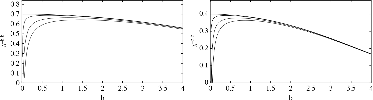
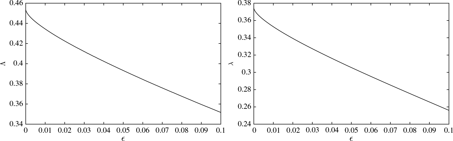
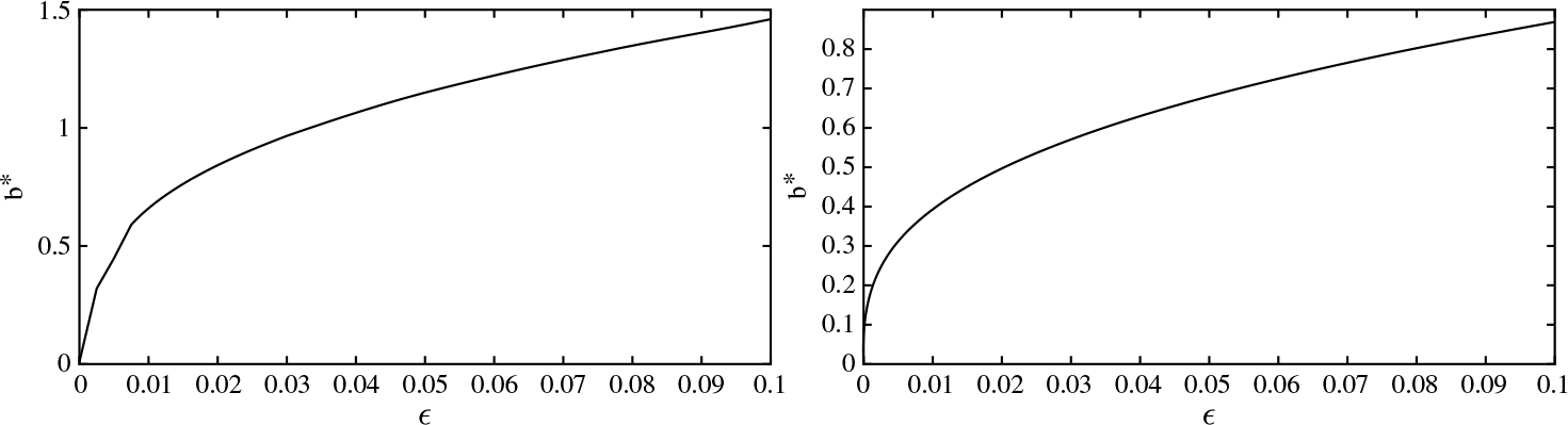
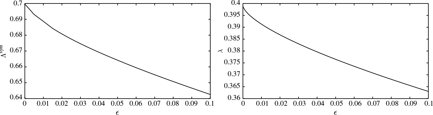
For a graphical illustration of how the symmetrical growth rate $\Lambda^{-b,b}$ varies with b for different transaction costs, see Figure 1 (left). Figures 2 (left) and 3 (left) show how the optimal threshold $b^*$ and the optimal growth rate $\Lambda$ vary with the slippage cost ${\varepsilon}$ , respectively.

Figure 1:

A plot of $\Lambda^{-b,b}$ (left) and $\lambda^{-b,b}$ (right) for $\varepsilon =[0, 0.01, 0.05, 0.10]$ . The parameters are $\beta =0.5$ and $\sigma=2$ . Note that $\Lambda^\textrm{sym} \geq \beta$ in this setting and hence $\Lambda=\Lambda^\textrm{sym}$ .

Figure 2:

The optimal threshold $b^*$ for the multiplicative version (left) and for the additive version (right) as a function of the slippage cost ${\varepsilon}$ . The remaining parameters are as in Figure 1.

Figure 3:

The optimal growth rate $\Lambda$ (left) and the optimal expected growth rate $\lambda$ (right) as a function of the slippage cost ${\varepsilon}$ . The remaining parameters are as in Figure 1. The graphs support the findings of Proposition 1.

4.2. Maximizing the expected growth rate

We now continue the study of the additive version suggested in Section 2.2. Denote by $\Delta^{ab}$ the time it takes for the process X, started at a, to reach b and then return to a. Then $\textrm{E}[\Delta^{ab}]=\textrm{E}_a[\tau_b] + \textrm{E}_b[\tau_a]$ . Next, let

\begin{equation*}u(x)\,:\!=\frac{2}{\sigma^2}\int_x^b\int_{-\infty}^y \frac{\varphi(y)}{\varphi(z)}\,\textrm{d} z\,\textrm{d} y,\end{equation*}

where $\varphi(y)=\exp\left\{\beta y^2/\sigma^2\right\},$ and note that

\begin{equation*}\left\{\begin{array}{ll} \frac{\sigma^2}{2}u''-\beta xu'+1=0, & \quad x<b,\\ u(b)=0.\end{array}\right.\end{equation*}

It is then straightforward to check that $u(x)=\textrm{E}_x[\tau_b]$ (with a similar result for $\textrm{E}_x[\tau_a]$ ). Consequently,

(12) \begin{eqnarray} \textrm{E}[\Delta^{ab}]\ &=&\ \frac{2}{\sigma^2}\int_a^b\int_{-\infty}^y \frac{\varphi(y)}{\varphi(z)}\,\textrm{d} z\,\textrm{d} y + \frac{2}{\sigma^2}\int_a^b\int^{\infty}_y \frac{\varphi(y)}{\varphi(z)}\,\textrm{d} z\,\textrm{d} y\\[-25pt]\nonumber\end{eqnarray}

\begin{eqnarray} \notag &\ \ \ \ \ =\ &\frac{2}{\sigma^2}\int_a^b\int_{-\infty}^{\infty} \frac{\varphi(y)}{\varphi(z)}\,\textrm{d} z\,\textrm{d} y=\frac{2\sqrt{\pi}}{\sigma \sqrt{\beta}} \int_a^b \varphi(y)\,\textrm{d} y, \end{eqnarray}

where we used that

\begin{equation*}\int_{-\infty}^{\infty} \textrm{e}^{-x^2}\,\textrm{d} x=\sqrt{\pi}.\end{equation*}

By (3) and Theorem 2, the long-term expected growth rate of a strategy (a, b) is given by

(13) \begin{equation} \lambda^{ab}=\frac{\ln((1-{\varepsilon})e^{b-a})}{\textrm{E}[\Delta^{ab}]}=\frac{\ln(1-{\varepsilon})+b-a}{\textrm{E}[\Delta^{ab}]}. \end{equation}

Theorem 4. Let $b^*$ be the unique positive solution of

(14) \begin{equation} 2\int_0^b \varphi(y)\,\textrm{d} y=(2b+\ln (1-{\varepsilon}))\varphi(b), \end{equation}

and set

\begin{equation*}\lambda\,:\!= \frac{\sigma \sqrt{\beta}}{2\sqrt{\pi} \varphi(b^*)}.\end{equation*}

Then the strategy $(a,b)\,:\!=(-b^*,b^*)$ is optimal in (13), and $\lambda$ is the corresponding optimal expected growth rate.

Proof. It is clear from (12) that for a given distance $k>0$ between a and b the mean cycle time $\Delta^{ab}=\Delta^{b-k,b}$ is minimized at $b=k/2$ . Consequently, the quotient $\lambda^{ab}$ in (13) is maximized for $a=-b$ , and we are thus left to maximize

\begin{equation*} \lambda(b)\,:\!=\lambda^{-b,b}=\frac{\sigma \sqrt{\beta}(2b+\ln(1-{\varepsilon}))}{4\sqrt{\pi} \int_0^b \varphi(y)\,\textrm{d} y } \end{equation*}

over $b\geq 0$ . Note that $\lambda(0+)=-\infty$ , $\lambda(\infty)=0$ , and $\lambda(b)> 0$ for all $b> \frac{1}{2}\ln\frac{1}{1-{\varepsilon}}$ , so by continuity, $\lambda(b)$ has a maximum. Moreover, the first-order condition $\lambda'(b)=0$ gives the equation (14). Equation (14) has a unique positive solution since the function

\begin{equation*}f(b)\,:\!=2\int_0^b \varphi(y)\,\textrm{d} y-(2b+\ln (1-{\varepsilon}))\varphi(b)\end{equation*}

satisfies $f(0)>0$ , $f'(b)\geq 0$ for $b\in\big(0,\frac{1}{2}\ln\frac{1}{1-{\varepsilon}}\big)$ and $f'(b)<0$ for $b\in\big(\frac{1}{2}\ln\frac{1}{1-{\varepsilon}},\infty\big)$ with $f'(b)\to-\infty$ as $b\to\infty$ . Hence the solution of (14) gives the maximal expected growth rate.

Finally, the maximal expected growth rate is given by

\begin{equation*}\lambda(b^*)=\frac{\sigma \sqrt{\beta}(2b^*+\ln(1-{\varepsilon}))}{4\sqrt{\pi} \int_0^{b^*} \varphi(y)\,\textrm{d} y }= \frac{\sigma \sqrt{\beta}}{2\sqrt{\pi} \varphi(b^*)},\end{equation*}

where (14) is used for the second equality.\hfill $\square$

For a graphical illustration of how the expected growth rate $\lambda^{-b,b}$ varies with b for different slippage costs, see Figure 1 (right). For the dependence in the optimal strategy on the slippage cost, see Figure 2 (right), and for an illustration of how the maximal expected growth rate decays, see Figure 3 (right).

5.1. Maximizing the growth rate of the expected return

In the multiplicative version we look for $\Lambda=\Lambda^{ab}$ satisfying

\begin{equation*}\textrm{E}_a[\exp\{-\Lambda \tau_b\}] \textrm{E}_b\left[\exp\left\{\int_0^{\tau_a}\hat \mu(t)\,\textrm{d} t -\frac{\sigma^2}{2}\tau_a+\sigma \hat W(\tau_a)-\Lambda \tau_a\right\}\right]=\frac{1}{1-{\varepsilon}},\end{equation*}

cf. Theorem 1. By a Girsanov change of measure, this is equivalent to finding $\Lambda$ such that

(15) \begin{equation} \textrm{E}_a[\exp\{-\Lambda \tau_b\}] \tilde{\textrm{E}}_b\left[\exp\left\{\int_0^{\tau_a}\hat \mu(t)\,\textrm{d} t -\Lambda \tau_a\right\}\right]=\frac{1}{1-{\varepsilon}}, \end{equation}

where $\Pi$ now satisfies

\begin{equation*}\textrm{d}\Pi(t)=(\lambda_1(1-\Pi_t)-\lambda_2\Pi_t+\sigma\omega\Pi(t)(1-\Pi(t)))\,\textrm{d} t +\omega\Pi_t(1-\Pi_t)\, \textrm{d}\tilde W(t)\end{equation*}

and $\tilde W$ is a Brownian motion under a new measure $\tilde {\mathbb P}$ .

We have not been able to find explicit expressions for the two expected values on the left-hand side of (15). Instead, the optimization problem is solved numerically. To treat the first expected value in (15), note that for each fixed $b\in(0,1)$ , the function $u(\pi)\,:\!=\textrm{E}_\pi[\exp\{-\Lambda \tau_b\}]$ is the unique solution of the ordinary differential equation

(16) \begin{equation} \left\{\begin{array}{ll} \frac{\omega^2\pi^2(1-\pi)^2}{2}u'' + (\lambda_1-(\lambda_1+\lambda_2)\pi)u'-\Lambda u=0,\quad &\quad \pi\in(0,b),\\[3pt] u(b)=1,\\[3pt] \lambda_1 u'(0)=\Lambda u(0)\end{array}\right. \end{equation}

(here, the boundary condition at $\pi=0$ is obtained by inserting $\pi=0$ in the ordinary differential equation). However, rather than solving the system (16) for each b and $\Lambda$ , we instead solve

\begin{equation*} \left\{\begin{array}{ll} \frac{\omega^2\pi^2(1-\pi)^2}{2}v'' + (\lambda_1-(\lambda_1+\lambda_2)\pi)v'-\Lambda v=0, &\quad \pi\in(0,1),\\[3pt] v(0)=1,\\[3pt] \lambda_1 v'(0)=\Lambda v(0)\end{array}\right. \end{equation*}

for different $\Lambda$ and note that $u(x)=\frac{v(x)}{v(b)}$ . A similar remark applies to the second factor on the left-hand side of (15).

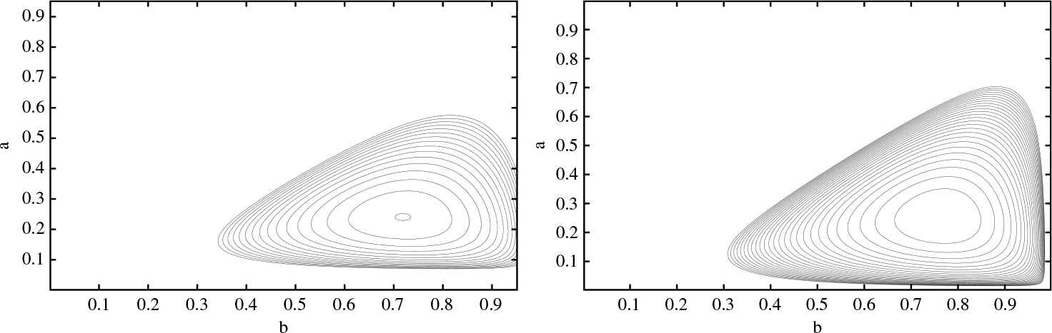
For a graphical illustration of the level curves of the function $\Lambda=\Lambda^{ab}$ , see Figure 4 (left). For an illustration how the optimal $\Lambda$ depends on the slippage cost ${\varepsilon}$ , see Figure 5 (left).

Figure 4:

Level curves of $\Lambda=\Lambda^{ab}$ (left) and of $\lambda=\lambda^{ab}$ (right). Here the parameters are $\mu_1=-1$ , $\mu_2=1$ , $\lambda_1=\lambda_2=2$ , $\sigma=0.2$ , and ${\varepsilon}=0.01$ .

Figure 5:

The optimal growth rate $\Lambda$ (left) and the optimal expected growth rate $\lambda$ (right) as a function of the slippage cost ${\varepsilon}$ . The remaining parameters are as in Figure 4.

5.2. Maximizing the expected rate of return

In view of Theorem 2, in order to maximize the expected rate of return we need to find $a<b$ which maximizes

(17) \begin{align} \lambda=\lambda^{ab}&\,:\!=\frac{\ln(1-{\varepsilon}) +\textrm{E}_b\big[ \int_0^{\tau_a}\hat \mu(t)\,\textrm{d} t -\frac{\sigma^2}{2}\tau_a\big]}{\textrm{E}_b[\tau_a]+\textrm{E}_a[\tau_b]} \notag\\[3pt] & = \frac{\ln(1-{\varepsilon})+\int_a^b\int_x^1\frac{\mu_1-\frac{\sigma^2}{2}+(\mu_2-\mu_1)y}{\alpha(y)}\exp\big\{\int_x^y\frac{\beta(z)}{\alpha(z)}\,\textrm{d} z\big\}\,\textrm{d} y\,\textrm{d} x} {\int_a^b\int_x^1\frac{1}{\alpha(y)}\exp\big\{\int_x^y\frac{\beta(z)}{\alpha(z)}\,\textrm{d} z\big\}\,\textrm{d} y\,\textrm{d} x + \int_a^b\int_0^x\frac{1}{\alpha(y)}\exp\big\{\int_x^y\frac{\beta(z)}{\alpha(z)}\,\textrm{d} z\big\}\,\textrm{d} y\,\textrm{d} x} \notag\\[3pt] & = \frac{\ln(1-{\varepsilon})+\int_a^b\int_x^1\frac{\mu_1-\frac{\sigma^2}{2}+(\mu_2-\mu_1)y}{\alpha(y)}\exp\big\{\int_x^y\frac{\beta(z)}{\alpha(z)}\,\textrm{d} z\big\}\,\textrm{d} y\,\textrm{d} x} {\int_0^1\frac{1}{\alpha(y)}\int_a^b\exp\big\{\int_x^y\frac{\beta(z)}{\alpha(z)}\,\textrm{d} z\big\}\,\textrm{d} x\,\textrm{d} y }, \end{align}

where $\beta(z)=\lambda_1-(\lambda_1+\lambda_2)z$ and $\alpha(z)=\omega^2z^2(1-z)^2/2$ . We cannot find any symmetries, so we believe that the optimization problem is inherently two-dimensional.

For a graphical illustration of the optimization in (17), see Figure 4 (right) and Figure 5 (right), in which the level curves of $\lambda^{ab}$ and the optimal growth rate $\lambda=\lambda({\varepsilon})$ are plotted.