1 Introduction
Understanding the dynamical behaviour of fibre-like objects dispersed in fluid flow is a relevant issue concerning many environmental and industrial processes, such as pollutant dispersion, microfluidic processing and paper production (du Roure et al. Reference du Roure, Lindner, Nazockdast and Shelley2019). Compared with point-like particles, the dynamics of fibres or, more generally, non-spherical particles, turns out to be more complex due to the additional degrees of freedom related to orientation, so that active research is devoted to improve the comprehension of such fluid–structure interactions.
In the case of rigid particles with ellipsoidal shape and which are sufficiently small to evolve in a Stokes flow with negligible fluid inertia, an analytical expression for the fluid torque acting on the particle was originally derived by Jeffery (Reference Jeffery1922). Such a result has been later generalized to other shapes and widely exploited in a variety of problems. These include studies on the rheology of suspensions in low-Reynolds-number flow conditions (Butler & Snook Reference Butler and Snook2018), as well as on the dynamics of dispersed fibres in turbulent flows (Voth & Soldati Reference Voth and Soldati2017). Focusing on the latter framework, several investigations concerned with both homogeneous isotropic turbulence (Parsa et al. Reference Parsa, Calzavarini, Toschi and Voth2012; Ni et al. Reference Ni, Kramel, Ouellette and Voth2015; Sabban, Cohen & van Hout Reference Sabban, Cohen and van Hout2017) as well as wall-bounded turbulent flows (Marchioli, Fantoni & Soldati Reference Marchioli, Fantoni and Soldati2010; Marchioli, Zhao & Andersson Reference Marchioli, Zhao and Andersson2016) reveal useful insights on the preferential alignment experienced by fibres and the correlation statistics between their orientation and vorticity. Additionally, Gustavsson et al. (Reference Gustavsson, Sheikh, Lopez, Naso, Pumir and Mehlig2019) recently focused on the settling of small prolate particles, while the orientation of rod-like particles in Taylor–Couette turbulence was analysed by Bakhuis et al. (Reference Bakhuis, Mathai, Verschoof, Ezeta, Lohse, Huisman and Sun2019).
Despite its significance, the approach based on Jeffery’s solution is justified only if the aforementioned assumptions are satisfied. For example, these no longer apply if the fibre length is larger than the Kolmogorov flow scale (i.e. the Reynolds number at the fibre length scale is not sufficiently small). In fact, the dynamical behaviour of fibres with length well within the inertial range of scales is far less understood and has been considered by only few recent experimental investigations (Bounoua, Bouchet & Verhille Reference Bounoua, Bouchet and Verhille2018; Kuperman, Sabban & van Hout Reference Kuperman, Sabban and van Hout2019), along with the numerical study of Do-Quang et al. (Reference Do-Quang, Amberg, Brethouwer and Johansson2014) who simulated rigid fibres of finite size in a turbulent channel flow. Furthermore, for Jeffery’s solution to hold strictly, it is also required that particle inertia (typically quantified by means of the Stokes number) can be neglected as well (Sabban et al. Reference Sabban, Cohen and van Hout2017).
A further breakdown for the application of Jeffery’s model is for the case of flexible fibres. The dynamics of flexible fibres in low-Reynolds-number flows has been recently reviewed by du Roure et al. (Reference du Roure, Lindner, Nazockdast and Shelley2019). For sufficiently small fibres, the typical modelling approach relies here on slender body theory (Cox Reference Cox1970; Tornberg & Shelley Reference Tornberg and Shelley2004). Using this approach, in particular, the motion of flexible fibres in cellular flows has been extensively studied by Young & Shelley (Reference Young and Shelley2007), Wandersman et al. (Reference Wandersman, Quennouz, Fermigier, Lindner and du Roure2010) and Quennouz et al. (Reference Quennouz, Shelley, Du Roure and Lindner2015), revealing the existence of flow-induced buckling instabilities that are responsible for their complex dynamics, including the possibility of a diffusive behaviour for neutrally buoyant fibres due to such deformation. Moreover, Allende, Henry & Bec (Reference Allende, Henry and Bec2018) recently investigated the stretching rate and buckling probability of non-inertial flexible fibres in ideal turbulence.
For flexible fibres with finite size, some recent contributions have considered this kind of object as the key ingredient for a novel way of flow measurement. In particular, the possibility of using flexible fibres to quantify two-point statistics has been highlighted by Rosti et al. (Reference Rosti, Banaei, Brandt and Mazzino2018a, Reference Rosti, Olivieri, Banaei, Brandt and Mazzino2020) in the case of homogeneous isotropic turbulence by means of fully resolved direct numerical simulation. This latter case is very far from the realm of application of Jeffery’s model for at least three main reasons. The fibres are elastic, inertial and they do not evolve locally in a linear flow (i.e. their size is well within the inertial range of scales). In this situation, the existence of different fibre flapping states was identified, in some of which the fibre behaves as a proxy of turbulent eddies with size comparable to the fibre length. Two-point statistical quantities, such as the velocity structure functions, were thus acquired simply by tracking the fibre end points in time. Related to this framework, significant contributions regarded the flapping instabilities of flexible filaments interacting with two-dimensional low-Reynolds-number flow (Shelley & Zhang Reference Shelley and Zhang2011), and similar mechanisms were explored for the purpose of passive locomotion and flow control purposes (Bagheri, Mazzino & Bottaro Reference Bagheri, Mazzino and Bottaro2012; Lācis et al. Reference Lācis, Brosse, Ingremeau, Mazzino, Lundell, Kellay and Bagheri2014, Reference Lācis, Olivieri, Mazzino and Bagheri2017). Along a similar line of reasoning, Hejazi, Krellenstein & Voth (Reference Hejazi, Krellenstein and Voth2019) investigated experimentally how to measure fluid velocity gradients using particles made by connections of slender deformable arms, both in the case of two-dimensional (2-D) shear flow and three-dimensional (3-D) turbulence.
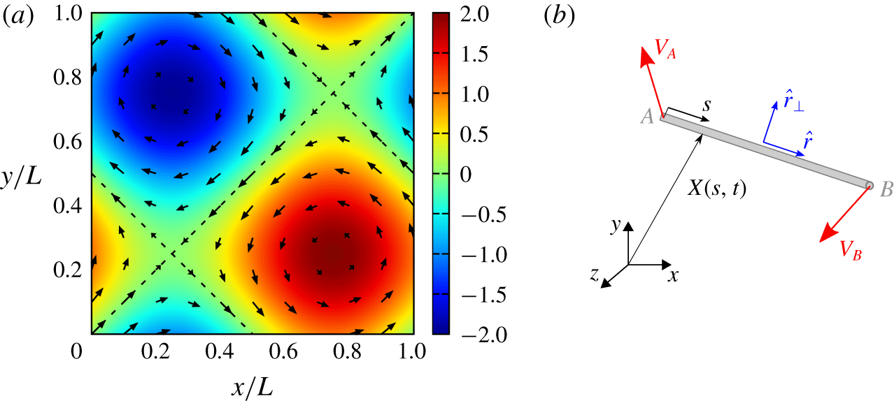
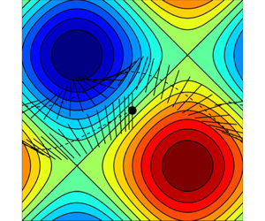
(a) The so-called BC cellular flow (the colourmap showing the stream function given by (3.1) along with the corresponding velocity vectors); (b) sketch of a generic fibre configuration (the characteristic quantities here indicated are introduced in the text).

Motivated by the evidence reported by Rosti et al. (Reference Rosti, Banaei, Brandt and Mazzino2018a, Reference Rosti, Olivieri, Banaei, Brandt and Mazzino2020), the goal of this work is to investigate similar possibilities for the case of rigid fibres in laminar flow. Rigid fibres are indeed easier to fabricate than elastic ones and are good candidates for novel experimental, non-invasive techniques able to access small-scale, multi-point properties of fluid flows. The idea is to replace single particles, typically used in particle image or tracking velocimetry (PIV/PTV) to measure single-point fluid properties (Adrian Reference Adrian1991; Hoyer et al. Reference Hoyer, Holzner, Lüthi, Guala, Liberzon and Kinzelbach2005; Schanz, Gesemann & Schröder Reference Schanz, Gesemann and Schröder2016), by single fibres (or assemblies of them) in order to access two-point (or multi-point) properties.
To this aim, we will focus on cellular flows, which are also a conceptual representation of eddies of turbulent flows. We will therefore consider spatially periodic solutions of the incompressible Navier–Stokes equations, i.e. the so-called Arnold–Beltrami–Childress (ABC) and Beltrami–Childress (BC) flows (Dombre et al. Reference Dombre, Frisch, Greene, Hénon, Mehr and Soward1986; Biferale et al. Reference Biferale, Crisanti, Vergassola and Vulpiani1995). A visualization of the latter is given in figure 1(a). The choice of this setting will enable us to perform a direct and reliable comparison between the measured fibre velocity and the underlying, unperturbed fluid flow velocity. Although the fibre velocity is generally different from the unperturbed fluid velocity, we will show that the velocities at fibre ends can be used to measure the velocity differences of the unperturbed fluid flow. With unperturbed velocity here we mean the velocity field of the flow in the absence of the fibre. In this framework, a new way for measuring the fluid velocity gradient tensor will be proposed and tested exploiting the assembly of different fibres (three fibres for the two-dimensional incompressible case and eight fibres for the corresponding three-dimensional case). Accessing the velocity gradient is of particular importance when dealing with turbulent flows, since from this quantity one can thus construct the vorticity and strain rate tensors, as well as obtaining the energy dissipation rate and other small-scale quantities.
It is worth summarizing in which sense our model for the fibre dynamics is different with respect to the well known Jeffery’s model. In our model the fibre is fully coupled to the flow and it will be of finite size, i.e. its length will be up to the typical size of the cellular flows we will consider. In general, the fibre will thus not be evolving in a linear flow as it is in the Jeffery’s model. Moreover, our fibre will be inertial. Different Stokes numbers will be analysed with the final aim of understanding up to which Stokes numbers a rigid fibre can be used as a proxy of unperturbed flow properties.
Following this introduction, the rest of the paper is structured as follows. In § 2 we present the numerical methods used in the work (complemented by appendix A), § 3 gives the results, and finally § 4 draws some conclusions and perspectives.
2 Methods
We consider an inertial, elastic fibre of length  $c$ and diameter
 $d\ll c$, characterized by (non-dimensional) linear density
 $\unicode[STIX]{x1D70C}_{1}$ and bending stiffness
 $\unicode[STIX]{x1D6FE}$. Given the position of a material point belonging to the fibre
 $\boldsymbol{X}=\boldsymbol{X}(s,t)$, as a function of the curvilinear coordinate
 $s$ and time
 $t$, the fibre dynamics is governed by the Euler–Bernoulli’s beam equation
 $$\begin{eqnarray}\unicode[STIX]{x1D70C}_{1}\ddot{\boldsymbol{X}}=\unicode[STIX]{x2202}_{s}(T\unicode[STIX]{x2202}_{s}(\boldsymbol{X}))-\unicode[STIX]{x1D6FE}\unicode[STIX]{x2202}_{s}^{4}(\boldsymbol{X})-\boldsymbol{F}.\end{eqnarray}$$
In (2.1),  $\boldsymbol{F}$ is the forcing exerted by the fluid–structure coupling, while
 $T$ is the tension necessary to enforce the inextensibility condition
 $$\begin{eqnarray}\unicode[STIX]{x2202}_{s}(\boldsymbol{X})\boldsymbol{\cdot }\unicode[STIX]{x2202}_{s}(\boldsymbol{X})=1.\end{eqnarray}$$
The fibre is freely moving in the flow, hence the corresponding boundary conditions at its ends are
 $$\begin{eqnarray}\unicode[STIX]{x2202}_{ss}\boldsymbol{X}|_{s=0,c}=\unicode[STIX]{x2202}_{sss}\boldsymbol{X}|_{s=0,c}=0,\end{eqnarray}$$
 $$\begin{eqnarray}T|_{s=0,c}=0.\end{eqnarray}$$
Nevertheless, we focus here on rigid fibres, as sketched in figure 1(b). To this end, throughout the work we choose and retain  $c/L=(2\unicode[STIX]{x03C0})^{-1}$ and
 $\unicode[STIX]{x1D6FE}=10$ for which we have an essentially rigid behaviour with negligible deformations. The latter can be quantified by looking at the magnitude of the end to end distance, which is always smaller than
 $\mathit{O}(10^{-8})$.
The fibre is discretized along  $s$ into segments with spatial resolution
 $\unicode[STIX]{x0394}s=c/(N_{L}-1)$, with
 $N_{L}$ being the number of Lagrangian points. To model the fluid–structure coupling, we will consider two different strategies: (i) a fully resolved approach where the feedback is taken into account (which will therefore be denoted as active) and (ii) an intrinsically passive model based on slender body theory. Both strategies are introduced later in this section.
2.1 Active model
In the first case the coupling is two-way and the dynamics is resolved using an immersed boundary (IB) technique, inspired by the method proposed by Huang, Shin & Sung (Reference Huang, Shin and Sung2007) for anchored filaments in laminar flow. The method was also exploited for dispersed fibres in turbulent flow (Rosti et al. Reference Rosti, Banaei, Brandt and Mazzino2018a, Reference Rosti, Olivieri, Banaei, Brandt and Mazzino2020; Banaei, Rosti & Brandt Reference Banaei, Rosti and Brandt2020). In the present case, we solve numerically the incompressible Navier–Stokes equations for the fluid flow (details on the solution method can be found in appendix A),
 $$\begin{eqnarray}\displaystyle & \displaystyle \unicode[STIX]{x2202}_{t}\boldsymbol{u}+\boldsymbol{u}\boldsymbol{\cdot }\boldsymbol{\unicode[STIX]{x2202}}\boldsymbol{u}=-\boldsymbol{\unicode[STIX]{x2202}}p/\unicode[STIX]{x1D70C}_{0}+\unicode[STIX]{x1D708}\unicode[STIX]{x2202}^{2}\boldsymbol{u}+\boldsymbol{f}, & \displaystyle\end{eqnarray}$$
 $$\begin{eqnarray}\displaystyle & \displaystyle \boldsymbol{\unicode[STIX]{x2202}}\boldsymbol{\cdot }\boldsymbol{u}=0, & \displaystyle\end{eqnarray}$$
where  $\boldsymbol{u}$ is the fluid velocity,
 $p$ the pressure,
 $\unicode[STIX]{x1D70C}_{0}$ the density and
 $\unicode[STIX]{x1D708}$ the kinematic viscosity. The volumetric forcing
 $\boldsymbol{f}$ is made by the sum of two contributions: the first is used for generating the desired flow field (Dombre et al. Reference Dombre, Frisch, Greene, Hénon, Mehr and Soward1986), while the second is characteristic of the IB method, mimicking the presence of the fibre by means of no-slip enforcement at the Lagrangian points. Note that the single-mode non-random nature of the volume forcing considered here to generate the flow field does not require the special attention as for the cases considered, for example, by Chouippe & Uhlmann (Reference Chouippe and Uhlmann2015).
When using this approach, we consider a cubic domain of side  $L=2\unicode[STIX]{x03C0}$ with periodic boundary conditions in all directions, which is discretized into a uniformly spaced Cartesian grid using
 $N=64$ cells per side. The number of Lagrangian points describing the fibre is chosen in such a way that the Lagrangian spacing
 $\unicode[STIX]{x0394}s$ is almost equal to that of the Eulerian grid
 $\unicode[STIX]{x0394}x$; for example, for a fibre with length
 $c=1$ we use
 $N_{L}=11$ Lagrangian points. Doubling both resolutions, the variation of results was found to be negligible. As for the time step we use
 $\unicode[STIX]{x0394}t=5\times 10^{-5}$, after assessing the convergence for this parameter as well.
2.2 Passive model
In the second approach, a one-way coupling is assumed, i.e. the fibre is forced by the flow but not vice versa. The problem thus essentially consists in solving only (2.1), within which the forcing term is expressed as
 $$\begin{eqnarray}\boldsymbol{F}=\frac{\unicode[STIX]{x1D70C}_{1}}{\unicode[STIX]{x1D70F}_{s}}\,(\dot{\boldsymbol{X}}-\boldsymbol{u}(\boldsymbol{X}(s,t),t)),\end{eqnarray}$$
 $\unicode[STIX]{x1D70F}_{s}$ being the relaxation time of a fibre immersed in viscous flow, i.e. it can be identified with a Stokes time. Overall, it represents a measure of the fibre inertia compared to the flow, and also quantifies the strength of the coupling. In this approach,
 $\boldsymbol{u}$ is assigned and does not get modified by the presence of the fibre. Note that our model is similar (apart from the contribution of inertia that we have accounted for in our model) to that of Young & Shelley (Reference Young and Shelley2007) and Quennouz et al. (Reference Quennouz, Shelley, Du Roure and Lindner2015), relying on local slender body theory, and further simplified assuming an isotropic form for
 $\boldsymbol{F}$.
Using this model, we assess the convergence of the solution only with the Lagrangian resolution (since there is not the need for an Eulerian grid in this case) and the computational time step. Testing was performed for several initial positions of the fibre and in different cellular flow configurations (i.e. 2-D or 3-D, steady or oscillating). Given the substantially lower computational demand of this approach compared with the active model, for a fibre with length  $c=1$ we choose
 $N_{L}=31$ and
 $\unicode[STIX]{x0394}t=10^{-6}$, although a numerically stable and resolution-independent solution is already found with coarser resolution, accordingly with our findings for the active case.
3 Results
3.1 Two-dimensional BC flow
To start our analysis, we consider the steady and two-dimensional cellular flow, often named as the Beltrami–Childress flow, that is defined by the stream function
 $$\begin{eqnarray}\unicode[STIX]{x1D6F9}(x,y)=\sin (y)-\sin (x),\end{eqnarray}$$
which is shown in figure 1(a). From (3.1), it follows that the velocity field can be expressed as
 $$\begin{eqnarray}\left.\begin{array}{@{}c@{}}u=\cos y,\\ v=\cos x.\end{array}\right\}\end{eqnarray}$$
Such a relatively simple flow configuration will first be used for assessing the importance of fibre inertia by evaluating the rotational Stokes number, and then to present the actual method for measuring two-point velocity differences.
3.1.1 Rotational Stokes number
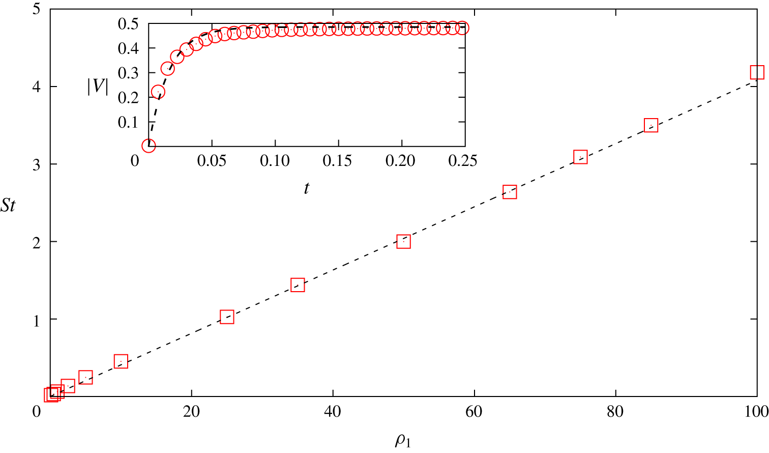
Rotational Stokes number as a function of fibre linear density. Red squares, measured values using the active model; black dashed line, linear fit. Inset: time history of the velocity magnitude of one fibre end (red circles) fitted using (3.3) (black dashed line), for a fibre with  $\unicode[STIX]{x1D70C}_{1}=0.1$.

As a preliminary step, we characterize the effect of fibre inertia by estimating the rotational Stokes number, which is the most suitable quantity to consider when dealing with cellular flows such as those considered in this work. This has been done for the sole active fibres, the Stokes number being an assigned parameter in the passive case as shown by (2.7).
To this end, we proceed as follows. We place the fibre at the centre of one cell in the BC flow (figure 1a). The fibre is initially at rest and, under the action of the flow, will start to purely rotate around its centre of mass. We measure the time it takes for the fibre to adapt to the flow, i.e. focusing on the velocity magnitude of one fibre end  $V(t)$, to assume constant velocity
 $V_{0}$ compatible with the unperturbed fluid velocity. Hence, we perform an exponential fit
 $$\begin{eqnarray}V(t)=V_{0}(1-\text{e}^{-t/\unicode[STIX]{x1D70F}_{s}})\end{eqnarray}$$
to measure the Stokes time  $\unicode[STIX]{x1D70F}_{s}$. An example of this procedure is given by the inset of figure 2. From the best fit we obtain the Stokes time and thus the Stokes number defined as
 $\mathit{St}=\unicode[STIX]{x1D70F}_{s}/\unicode[STIX]{x1D70F}_{f}$, where
 $\unicode[STIX]{x1D70F}_{f}=c/U$ is the characteristic hydrodynamic time scale (we choose
 $U=1$ as the flow velocity magnitude). The resulting behaviour of
 $\mathit{St}$ as a function of
 $\unicode[STIX]{x1D70C}_{1}$ is depicted in figure 2, showing that it can be well described by a linear law, as expected. Specifically, the best fit of
 $\mathit{St}$ versus
 $\unicode[STIX]{x1D70C}_{1}$ gives
 $\mathit{St}=\unicode[STIX]{x1D6FC}\unicode[STIX]{x1D70C}_{1}$ with
 $\unicode[STIX]{x1D6FC}\approx 0.04$.
Because in the beam equation only one relaxation time is involved in the passive case, its value has been identified as the rotational Stokes time measured in the active case.
3.1.2 Normal derivative of longitudinal velocity component
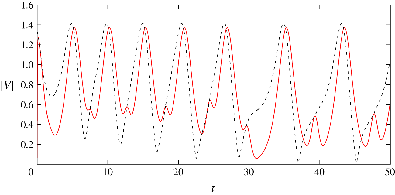
We are now ready to investigate the capability of a rigid fibre to act as a proxy of a laminar, cellular flow in terms of a few fibre properties such as its position and the velocity of the fibre end points. Figure 3 reports the velocity magnitude of one fibre end in time, compared with the velocity magnitude of the unperturbed flow (i.e. in the absence of the fibre) evaluated at the same point. It is evident that the two quantities differ appreciably. This result indicates that a fibre cannot be used to measure single-point flow quantities as done, for example in PIV techniques using tracer particles (Adrian Reference Adrian1991).
Velocity time series at one fibre end for the fibre (red solid line) and for the underlying unperturbed flow (black dashed line), for a fibre with  $\mathit{St}\approx 0.01$ released into the BC flow, computed with the active model.

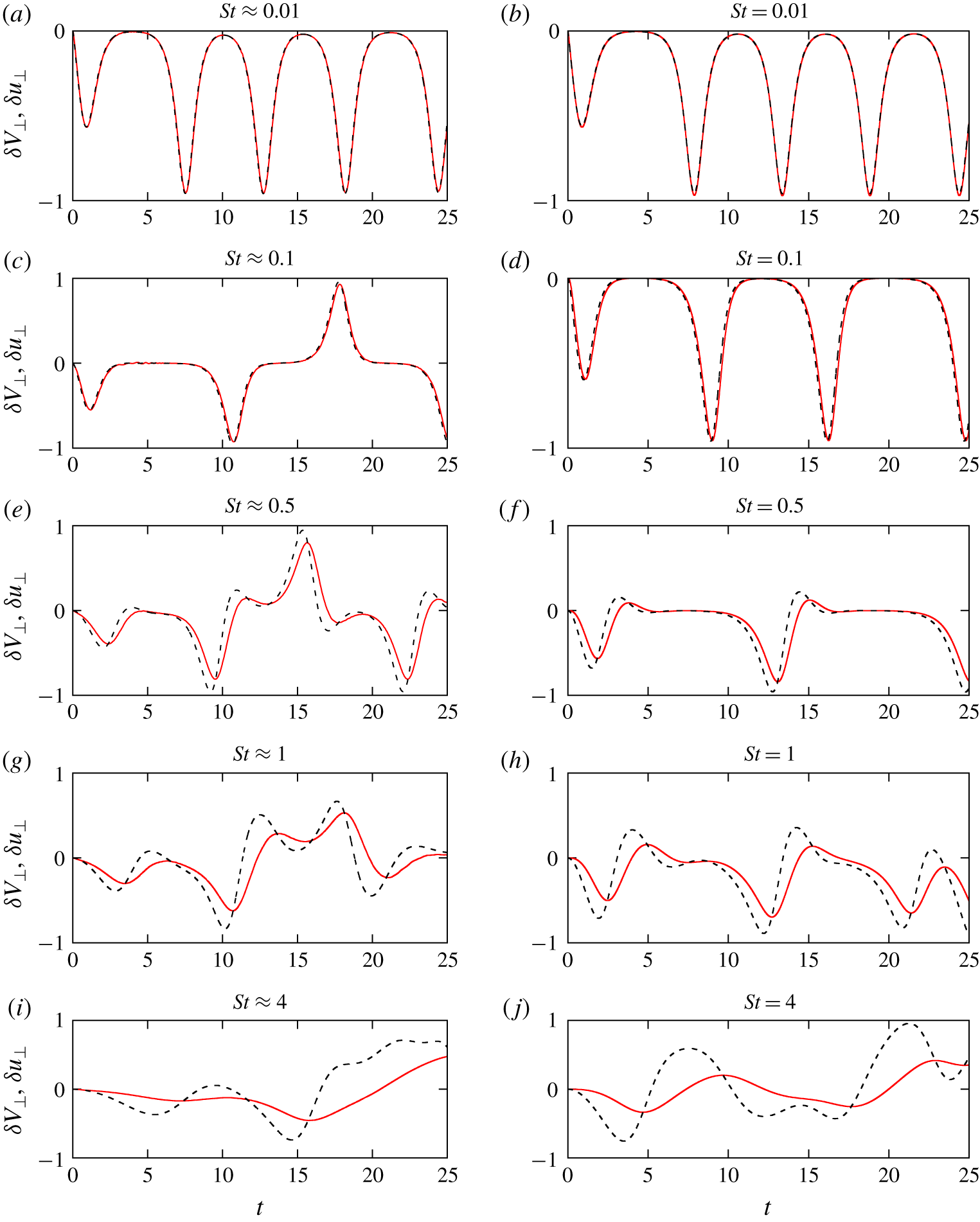
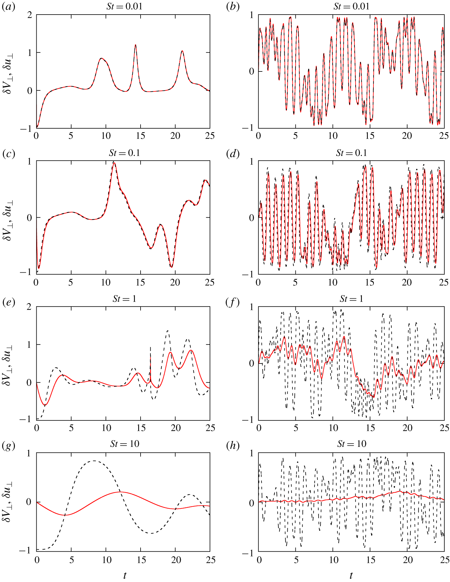
Transverse velocity differences of fibre  $\unicode[STIX]{x1D6FF}V_{\bot }$ (solid line) and unperturbed BC flow
 $\unicode[STIX]{x1D6FF}u_{\bot }$ (dashed line) for different Stokes number, both for the active (a,c,e,g,i) and passive (b,d,f,h,j) model. The normalized root mean square deviation between
 $\unicode[STIX]{x1D6FF}V_{\bot }$ and
 $\unicode[STIX]{x1D6FF}u_{\bot }$, for both active and passive model, is less than 1 % for
 $St\leqslant 0.1$, of the order of 10 % for
 $St\approx 0.5$ and larger than 15 % for
 $St\geqslant 1$. The fibre length is unity and it is thus approximately
 $32\,\%$ of the size of the single cell in the considered flow.

Hence, we consider the velocity difference between the fibre end points (figure 1b), i.e.  $\unicode[STIX]{x1D6FF}\boldsymbol{V}=\boldsymbol{V}_{B}-\boldsymbol{V}_{A}$, and denote by
 $\unicode[STIX]{x1D6FF}\boldsymbol{u}=\boldsymbol{u}|_{B}-\boldsymbol{u}|_{A}$ the corresponding unperturbed flow velocity difference. Comparing directly these two quantities, however, would still yield the same mismatch previously found for the velocity of one end. Such a mismatch is due not only to the fibre inertia, but also to the fibre inextensibility constraint. Indeed, if we consider the projection of the velocity difference introduced above along the direction parallel to the end to end distance,
 $\hat{\boldsymbol{r}}$, for a rigid and inextensible object, such a quantity is always zero, although the same quantity for the underlying unperturbed flow is clearly not. Our idea is then to project
 $\unicode[STIX]{x1D6FF}\boldsymbol{V}$ on a plane normal to
 $\hat{\boldsymbol{r}}$ by simply arguing that along that direction the effect of the inextensibility constraint should be washed out. In terms of the normal unit vector
 $\hat{\boldsymbol{r}}_{\bot }$ (shown in figure 1b), we define the projections,
 $$\begin{eqnarray}\displaystyle & \displaystyle \unicode[STIX]{x1D6FF}V_{\bot }=\unicode[STIX]{x1D6FF}\boldsymbol{V}\boldsymbol{\cdot }\hat{\boldsymbol{r}}_{\bot }, & \displaystyle\end{eqnarray}$$
 $$\begin{eqnarray}\displaystyle & \displaystyle \unicode[STIX]{x1D6FF}u_{\bot }=\unicode[STIX]{x1D6FF}\boldsymbol{u}\boldsymbol{\cdot }\hat{\boldsymbol{r}}_{\bot }. & \displaystyle\end{eqnarray}$$
The projected quantities (3.4) and (3.5) are compared in figure 4 where we report the results of our analysis in the BC flow configuration while varying  $\mathit{St}$, for both active and passive models. For relatively low
 $\mathit{St}$ (i.e. the first two rows of the figure), we now notice a remarkable agreement, i.e. the fibre is able to accurately measure the (unperturbed) flow transverse velocity increments in terms of its transverse velocity increments. For increasing
 $\mathit{St}$, i.e. the fibre inertia, the agreement gets worse, as expected. Overall, we observe a close resemblance between results for fibres starting from the same position, using the active (a,c,e,g,i) and passive (b,d,f,h,j) model, especially for the smallest
 $\mathit{St}$. This suggests that here the effective coupling between the flow and the fibre could be actually neglected, in relation to the measurement of transverse velocity differences. Accordingly, when extending our analysis to three-dimensional and unsteady flows (§ 3.2) we will exclusively employ the passive solver on the strength of such evidence.
Nevertheless, figure 4 tells us that the role of feedback cannot be entirely neglected. For sufficiently large Stokes numbers ( $\mathit{St}\geqslant 0.1$), the curves on the left panels, (c,e,g,i), and those on the right ones, (d,f,h,j), are different, revealing that the motion of the fibre centre of mass is affected by the feedback of the fibre to the flow. The effect of the latter is indeed crucial when the fibre centre of mass moves close to the flow separatrix, potentially causing totally different trajectories compared to the passive case.
Some further comments are worth considering. First, the projection along the normal direction to the fibre is crucial for the fibre to be a proxy of the flow velocity differences: if we project the velocity differences along a generic direction, the agreement shown before is no longer present (not shown here). In the two-dimensional case, the normal direction is uniquely defined by  $\hat{\boldsymbol{r}}_{\bot }=\pm (\hat{r}_{2},-\hat{r}_{1},0)$. In the three-dimensional case we have instead an infinite number of directions belonging to the normal plane to the fibre orientation. We retain
 $\hat{\boldsymbol{r}}_{\bot }=(\hat{r}_{2},-\hat{r}_{1},0)$ also for 3-D cases (see § 3.2) even if the results do not change for a different choice of
 $\hat{\boldsymbol{r}}_{\bot }$.
The situation considered in figure 4 refers to a fibre whose length is approximately  $32\,\%$ the size of the single cell. This is a case where the fibre length is sufficiently small compared to the variation scale of the flow. Under such condition the velocity difference between the free ends can be compared with the flow gradient evaluated at the fibre centre of mass. For the latter, the same projection along
 $\hat{\boldsymbol{r}}_{\bot }$ has to be applied as before. However, due to the tensorial structure of the gradient
 $\unicode[STIX]{x2202}_{j}u_{i}$, this translates to considering a double projection, first along the tangential and then along the normal direction,
 $$\begin{eqnarray}D=\unicode[STIX]{x2202}_{j}u_{i}\hat{r}_{j}\hat{r}_{i}^{\bot }.\end{eqnarray}$$
In figure 4, where  $c/L=(2\unicode[STIX]{x03C0})^{-1}$, the curve representing
 $D$ is not reported but would be essentially superimposed onto that of the fluid velocity difference. Doubling the fibre length, i.e.
 $c/L=\unicode[STIX]{x03C0}^{-1}$, the accuracy gets worse. This simply means that, despite the fact that the fibre accurately measures the transverse velocity differences across the fibre ends, the fibre is too long to allow the derivative to be well approximated by the ratio of the increments.
Finally, another aspect to be considered is the tendency of inertial particles to sample preferential zones of the flow, giving rise to peculiar features such as small-scale clustering of dilute suspensions. This phenomenon is well known and has been thoroughly investigated for spherical particles in turbulent flows (see, e.g. Eaton & Fessler (Reference Eaton and Fessler1994), Bec et al. (Reference Bec, Biferale, Boffetta, Celani, Cencini, Lanotte, Musacchio and Toschi2006) and Bec et al. (Reference Bec, Biferale, Cencini, Lanotte, Musacchio and Toschi2007)) and has also been observed for anisotropic particles (see Voth & Soldati (Reference Voth and Soldati2017) and references therein). While this mechanism could impact on the potential of using fibres as a proxy of the flow (i.e. measuring only certain regions of space), we highlight that decreasing the Stokes number, along with improving the measure in itself, assures us that at the same time preferential sampling is reduced.
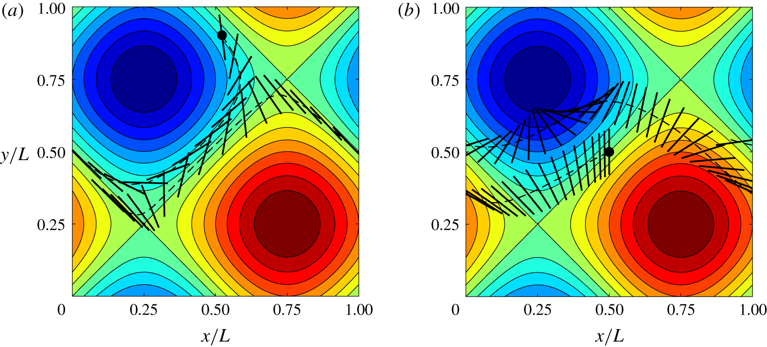
In steady cellular flows, we can easily observe the role of inertia in this regard by looking at the fibre trajectories and, in particular, their deviation from the flow streamlines. A visualization from our data is given in figure 5 where we compare two cases at different  $\mathit{St}$: the less inertial fibre with
 $\mathit{St}=0.1$ initially follows the cell streamlines but, due to the centrifugal effect, eventually reaches the flow separation lines (figure 5a), while the heavier fibre with
 $\mathit{St}=2$ shows a stronger deviation of its trajectory from the streamlines, resulting in a more diffusive behaviour (figure 5b).
Superposition of fibre positions at different instants within the periodic two-dimensional BC flow (the colourmap denoting the stream function), computed with the active model. (a)  $\mathit{St}=0.1$ and (b)
 $\mathit{St}=2$. The dashed line represents the trajectory of fibre centre of mass and the black circle indicates its starting position.

Transverse velocity differences of fibre  $\unicode[STIX]{x1D6FF}V_{\bot }$ (solid line) and unperturbed flow
 $\unicode[STIX]{x1D6FF}u_{\bot }$ (dashed line) for different Stokes numbers, computed using the passive model. (a,c,e,g) ABC flow (3.7); (b,d,f,h), 2-D oscillating cellular flow (equation (3.8)). The normalized root mean square deviation between
 $\unicode[STIX]{x1D6FF}V_{\bot }$ and
 $\unicode[STIX]{x1D6FF}u_{\bot }$, for both ABC flow and 2-D oscillating flow, is less than 1 % for
 $St\leqslant 0.1$, of the order of 15 % for
 $St=1$ and larger than 20 % for
 $St=10$.

3.2 Extension to three-dimensional and unsteady flows
As a further step, we test the capability of the fibre to measure the transverse velocity differences in three-dimensional steady or unsteady cellular flows. In light of our findings for the steady BC flow (§ 3.1), we present only results obtained with the passive model, although checks using the active model have been performed and yield the same overall scenario as in the steady, two-dimensional case.
First, we consider the so-called Arnold–Beltrami–Childress flow, which is known to be a time-independent, three-dimensional solution of Euler’s equations (Dombre et al. Reference Dombre, Frisch, Greene, Hénon, Mehr and Soward1986)
 $$\begin{eqnarray}\left.\begin{array}{@{}c@{}}u=\sin z+\cos y,\\ v=\sin x+\cos z,\\ w=\sin y+\cos x.\end{array}\right\}\end{eqnarray}$$
Unlike the two-dimensional BC flow previously considered, in this flow configuration the Lagrangian fluid elements show both regular and chaotic trajectories, depending on their initial position (Biferale et al. Reference Biferale, Crisanti, Vergassola and Vulpiani1995). A detailed analysis of this dynamical system can be found in Dombre et al. (Reference Dombre, Frisch, Greene, Hénon, Mehr and Soward1986).
In figure 6(a,c,e,g) we present the results of our analysis for this 3-D case. As for the BC flow, we find that for sufficiently low Stokes numbers, i.e.  $\mathit{St}\leqslant 0.1$, the agreement is evident between the fluid and fibre transverse velocity differences. Like the 2-D case and as expected, the agreement deteriorates for increasing
 $\mathit{St}$.
Next, we present the results for the unsteady, i.e. time-periodic, and two-dimensional flow
 $$\begin{eqnarray}\left.\begin{array}{@{}c@{}}u=\sin [x+\unicode[STIX]{x1D716}_{1}\sin (\unicode[STIX]{x1D714}_{1}t)]\cos [y+\unicode[STIX]{x1D716}_{2}\sin (\unicode[STIX]{x1D714}_{2}t)],\\ v=-\cos [x+\unicode[STIX]{x1D716}_{1}\sin (\unicode[STIX]{x1D714}_{1}t)]\sin [y+\unicode[STIX]{x1D716}_{2}\sin (\unicode[STIX]{x1D714}_{2}t)],\end{array}\right\}\end{eqnarray}$$
where  $\unicode[STIX]{x1D716}_{1}=\unicode[STIX]{x1D716}_{2}=0.2L$ are the amplitudes while
 $\unicode[STIX]{x1D714}_{1}=2\unicode[STIX]{x03C0}$ and
 $\unicode[STIX]{x1D714}_{2}=1$ are the frequencies of the oscillation along
 $x$ and
 $y$, respectively. This choice corresponds to a situation where the Lagrangian trajectories of fluid particles are chaotic (Castiglione et al. Reference Castiglione, Crisanti, Mazzino, Vergassola and Vulpiani1998; Cartwright et al. Reference Cartwright, Feudel, Károlyi, de Moura, Piro and Tél2010). The projected velocity differences are shown in figure 6(b,d,f,h), where the same conclusions drawn for steady configurations are confirmed: the agreement between the fibre-based measurement and the direct evaluation using the flow expression (3.8) increases by decreasing the rotational Stokes number.
3.3 Evaluation of the velocity gradient tensor
Having characterized the behaviour of single fibres, we can move further, focusing on how to access the full velocity gradient tensor  $\unicode[STIX]{x2202}_{j}u_{i}$ and not only its normal-directional projection. This will be achieved by assembling several fibres in a suitable way and exploiting the following idea: for each fibre, equation (3.6) holds, where the velocity gradient becomes the unknown variable if we use
 $\unicode[STIX]{x1D6FF}V_{\bot }$ (that is measured by tracking the fibre trajectory) in place of
 $D$. Considering an assembly made by
 $N_{f}$ fibres, we thus have a system of
 $N_{f}$ equations, from which the gradient can be obtained.
Let us therefore estimate the number of fibres that are needed in the two-dimensional case: here  $\unicode[STIX]{x2202}_{j}u_{i}$ is made by
 $2\times 2$ elements; however, the number of independent quantities is reduced of one by exploiting incompressibility. Hence, the assembly has to be made by
 $N_{f}=3$ fibres, yielding the following system to be solved:
 $$\begin{eqnarray}\left.\begin{array}{@{}c@{}}\unicode[STIX]{x1D6FF}V_{\bot }^{(1)}=\unicode[STIX]{x2202}_{j}u_{i}\hat{r}_{j}^{(1)}\hat{r}_{i}^{\bot (1)},\\[5.0pt] \unicode[STIX]{x1D6FF}V_{\bot }^{(2)}=\unicode[STIX]{x2202}_{j}u_{i}\hat{r}_{j}^{(2)}\hat{r}_{i}^{\bot (2)},\\[5.0pt] \unicode[STIX]{x1D6FF}V_{\bot }^{(3)}=\unicode[STIX]{x2202}_{j}u_{i}\hat{r}_{j}^{(3)}\hat{r}_{i}^{\bot (3)}.\end{array}\right\}\end{eqnarray}$$
In this system the final number of unknowns is three (i.e. three components of  $\unicode[STIX]{x2202}_{j}u_{i}$ out of four because of the incompressibility condition). Both the left-hand side of the equations and the coefficients of the velocity derivative tensor are easily measurable at each time step along the fibre trajectories and thus known from the numerical experiments. The system can be thus easily solved at each time step while following the fibre along its trajectory.
The three fibres will be connected at their centroids (numerically, it is convenient to realize these connections using springs with sufficiently high stiffness so that the distance between centroids is negligible). However, we shall let each fibre behave as in the single case, its dynamics not being substantially altered by the link with the others. To this end, it is crucial to avoid any rotational restraint, so that fibres are able to rotate freely with respect to each other. For the assembly, we measured the rotational Stokes number following the same procedure described in § 3.1.1 for the single fibre. The resulting relaxation times of each fibre composing the assembly turned out to be the same as the rotational Stokes time of the single isolated fibre. One can thus conclude that the Stokes time of the assembly is the same as that of a single fibre.
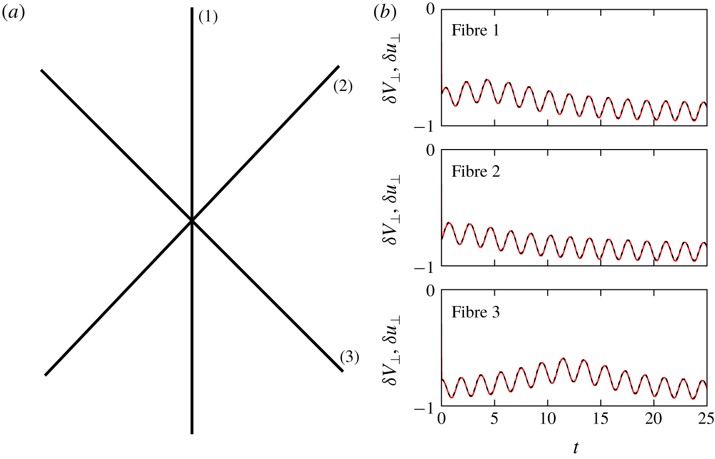
(a) Sketch of fibre assembly. (b) Transverse velocity differences of each fibre  $\unicode[STIX]{x1D6FF}V_{\bot }$ (solid line) and underlying unperturbed flow
 $\unicode[STIX]{x1D6FF}u_{\bot }$ (dashed line) in the case of BC flow with
 $c=1$ and
 $\mathit{St}\approx 0.01$, computed using the active model.

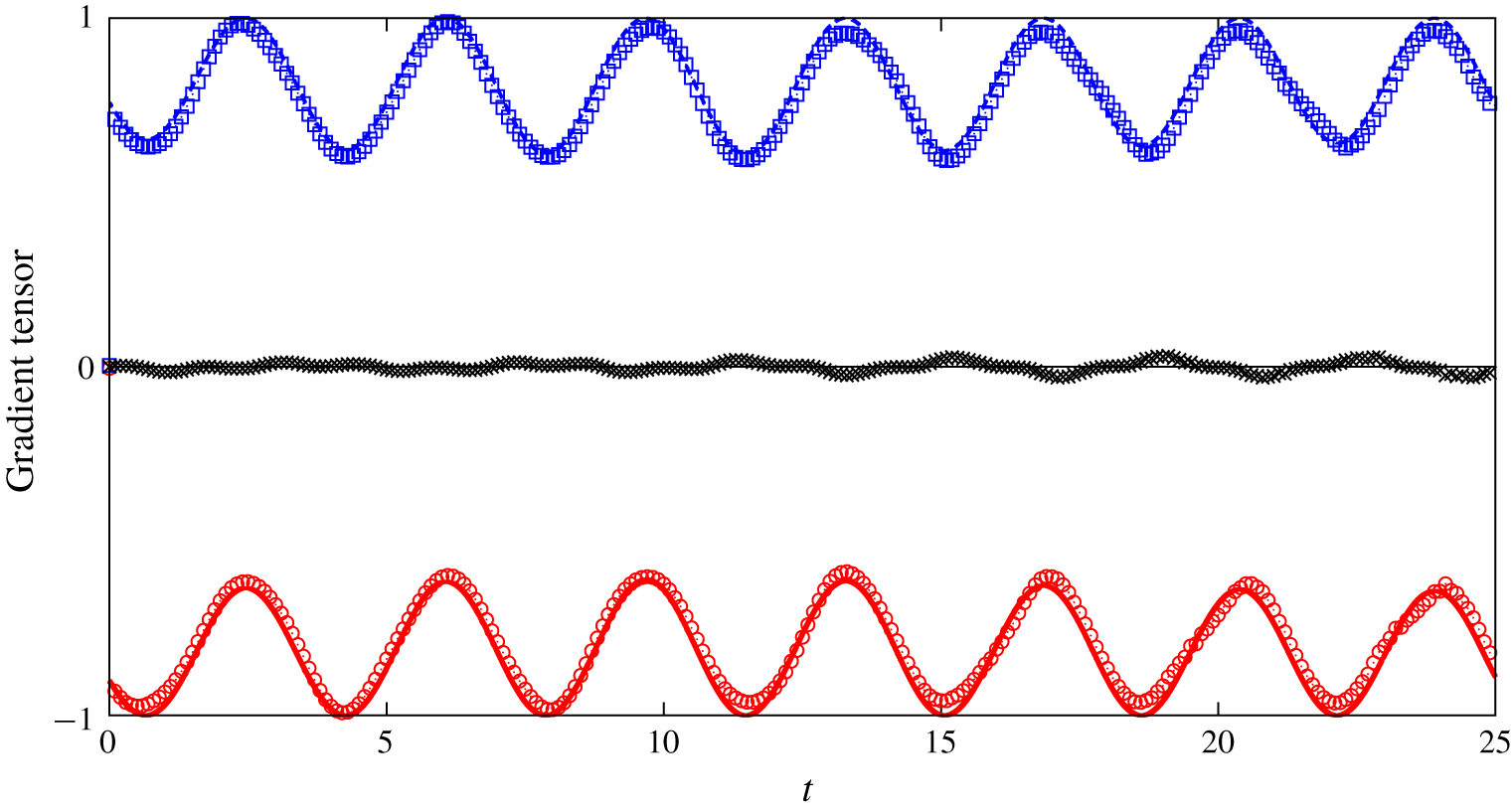
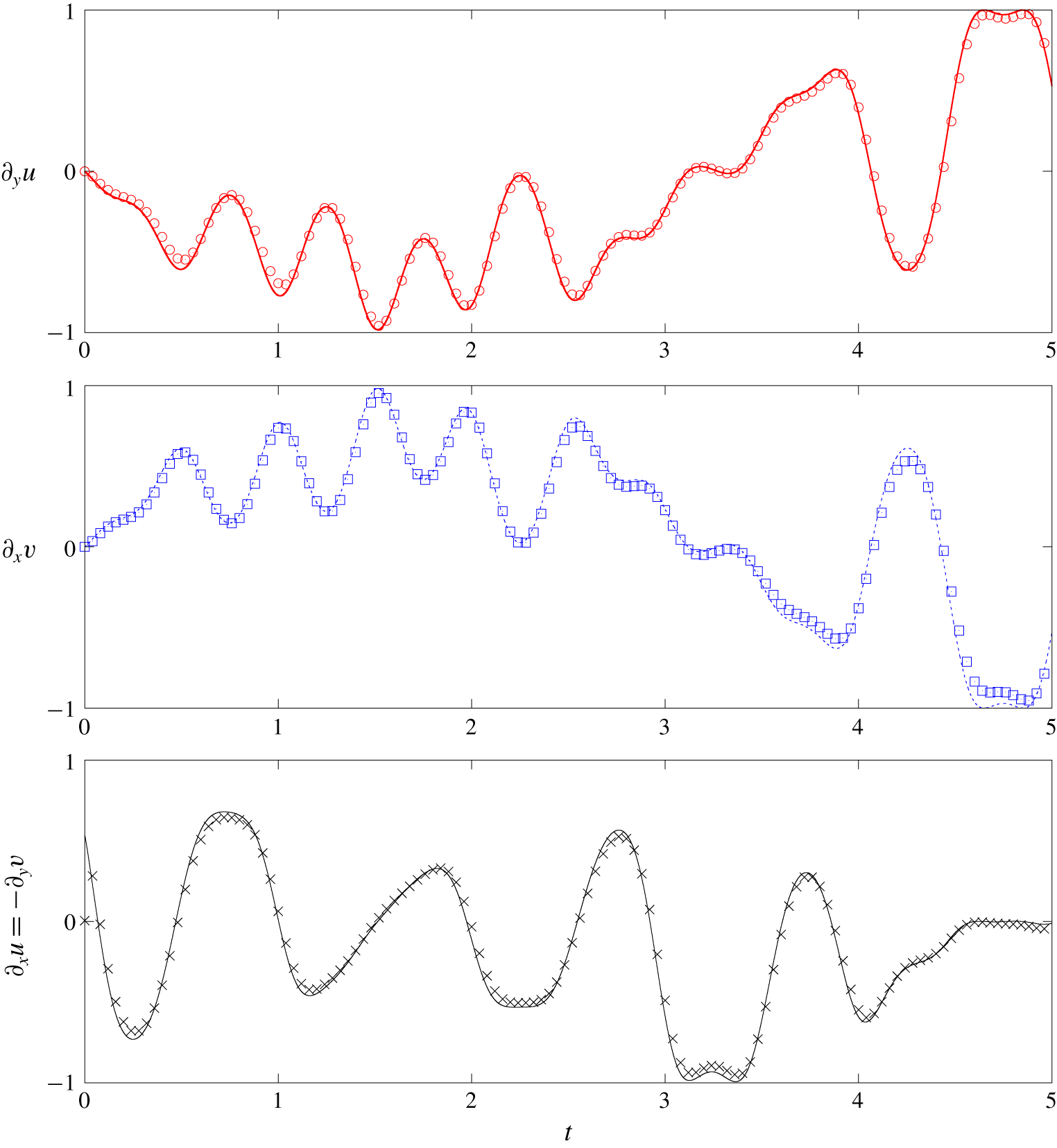
Velocity gradient tensor components in the BC flow (3.2) reconstructed by tracking the fibre assembly with  $\mathit{St}\approx 0.01$, using the active model. Red circles,
 $\unicode[STIX]{x2202}_{y}u$ obtained by the fibre Lagrangian tracking; red solid line,
 $\unicode[STIX]{x2202}_{y}u$ for the unperturbed flow; blue squares,
 $\unicode[STIX]{x2202}_{x}v$ obtained by the fibre Lagrangian tracking; blue dashed line,
 $\unicode[STIX]{x2202}_{x}v$ for the unperturbed flow; black crosses,
 $\unicode[STIX]{x2202}_{x}u=-\unicode[STIX]{x2202}_{y}v$ obtained by the fibre Lagrangian tracking; black line,
 $\unicode[STIX]{x2202}_{x}u=-\unicode[STIX]{x2202}_{y}v=0$ for the unperturbed flow. The normalized root mean square error between the components of the gradient tensor reconstructed by the Lagrangian tracking and those of the unperturbed flow is of the order of 1 %.

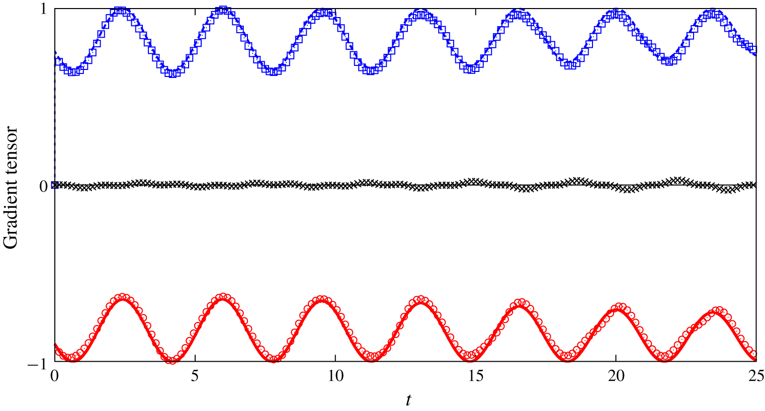
Now we are ready to test the outlined concept in the steady BC flow already used in § 3.1. As a first step, we look at the resulting time histories of the projected velocity difference for each fibre composing the assembly (figure 7), recovering the same evidence found in the case of single fibres. This provides a clue that also in this configuration it is possible to capture the features of the fluid flow. Indeed, we proceed to combine the information from all fibres, finally obtaining the velocity gradient tensor as shown in figure 8, where the time series of each element of  $\unicode[STIX]{x2202}_{j}u_{i}$ is reported, both for the fibre Lagrangian tracking and for the corresponding analytical value of the unperturbed flow. The comparison between the two quantities yields good agreement, with differences that are ascribed to numerical resolution and the finite inertia of fibres.
The reported results are for the active model but very similar evidence is obtained using the passive model. In figure 9 we show the result for the assembly of passive fibres in the static BC flow, highlighting essentially the same behaviour obtained in the active case (note that the same initial condition for the assembly of fibres was used in both cases). Finally, we complement the analysis by employing an assembly of passive fibres in the oscillating two-dimensional flow introduced in § 3.2, equation (3.8). Results are shown in figure 10 from which we can confirm the same conclusion as outlined before.
As in figure 8 but for assembly of passive fibres. The normalized root mean square error between the components of the gradient tensor reconstructed by the Lagrangian tracking and those of the unperturbed flow is of the order of 1 %.

As in figure 9 but for the oscillating two-dimensional flow (3.8) (the figure is split into three panels for a better readability of the gradient tensor components). The normalized root mean square error between the components of the gradient tensor reconstructed by the Lagrangian tracking and those of the unperturbed flow is of the order of 1 %.

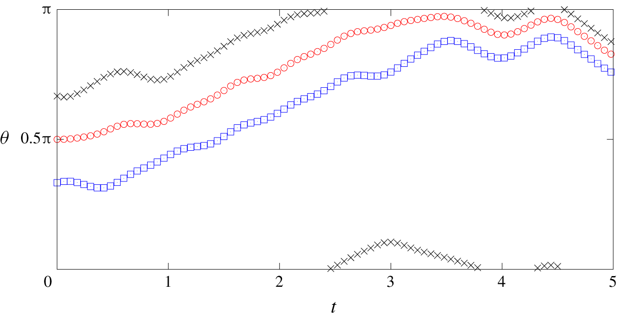
It is worth noting that the linear system (3.9) we numerically solved to obtain all components of the flow gradient can become overdetermined because of the alignment of two of more fibres. To avoid this problem we found that the simple recipe of imposing a small displacement (of  $\unicode[STIX]{x0394}s$, the size of the Lagrangian mesh) between the centroids of the fibres of the assembly (instead of imposing them to be zero) is enough to prevent perfect alignment of the fibres, thus preventing the breakdown of the solution. The results reported in figures 8–10 have been obtained exploiting this simple, but effective, strategy. Figure 11 reports the time history of the angle of the three fibres composing the assembly, in the oscillating two-dimensional flow. As shown in figure, in the considered time frame the alignment between the fibres does not occur and the minimum value of the standard deviation between the three angles is 0.18 rad. Extending the time frame (not shown), up to 25, the minimum value of the standard deviation we measured was 0.0085 rad which was, however, large enough to accurately solve the system.
Time history of the angles (rad) of the three fibres composing the assembly in the two-dimensional oscillating flow. Red circles, fibre 1; blue squares, fibre 2; black crosses, fibre 3. Angles are measured with respect to the horizontal direction. The minimum value of the standard deviation is  $0.18$.

4 Conclusions and perspectives
This study focused on the capability of measuring the whole structure of the velocity gradient in steady, unsteady regular and chaotic cellular flows by means of Lagrangian tracking of assembly of rigid fibres. Two different kinds of fibre models have been considered: a fully coupled fibre described in terms of an immersed-boundary method and a passive fibre described by the slender body theory. We first characterized the role of fibre inertia by defining a rotational Stokes number, which is evaluated as a function of the fibre linear density. Hence, considering the velocity difference between the fibre end points and the same difference concerning the underlying fluid velocity, both projected along the normal direction to the fibre, we showed that the fibre turns out to be a proxy of such two-point quantity. For sufficiently small fibres, this two-point quantity reduces to the transverse component of the flow velocity derivative along the fibre direction. Furthermore, the comparison between results obtained for the active model and the passive model suggests that the coupling between the flow and the fibre could be neglected, at least for small  $\mathit{St}$.
This capability of using rigid fibres as a way of measuring flow properties has potential applications in experimental techniques allowing us to access small-scale, multi-point properties of fluid flows, offering an alternative to other methods that have been proposed which rely on complex elaborations using PIV/PTV (Hoyer et al. Reference Hoyer, Holzner, Lüthi, Guala, Liberzon and Kinzelbach2005; Krug et al. Reference Krug, Holzner, Lüthi, Wolf, Tsinober and Kinzelbach2014; Lawson & Dawson Reference Lawson and Dawson2014). Future work will thus be devoted to the practical implementation of the outlined concept in a laboratory environment. Preliminary results in this direction considering rigid fibres of millimetric size dispersed in turbulent flow appear very encouraging (Brizzolara Reference Brizzolara2019), confirming the validity of our idea in a framework well beyond the laminar/chaotic examples analysed here. The applicability of the concept can thus be extended to three-dimensional and/or turbulent flows, along with considering assemblies of fibres that would be able to measure the full structure of the velocity gradient.
Acknowledgements
The authors warmly acknowledge A. A. Banaei, M. E. Rosti and L. Brandt (KTH, Sweden) for sharing an initial version of the code for the active solver. CINECA and INFN are also acknowledged for the availability of high performance computing resources and support. A.M. thanks the financial support from the Compagnia San Paolo, project MINIERA no. I34I20000380007.
Declaration of interests
The authors report no conflict of interest.
Appendix A. Immersed boundary method
This appendix presents the numerical procedure regarding the active approach introduced in § 2.1. The Navier–Stokes equations (2.5) and (2.6) are solved for a cubic domain of side  $L$ with periodic boundary conditions in all directions, which is discretized into a Cartesian grid using
 $N$ points per side. The solution is obtained by using a finite difference, fractional step method on a staggered grid with fully explicit space discretization and third-order Runge–Kutta scheme for advancement in time. Finally, the resulting Poisson equation enforcing incompressibility is solved using a fast Fourier transform.
As for the fibre-flow interaction, we employ the IB approach of Huang et al. (Reference Huang, Shin and Sung2007) and later modified by Banaei et al. (Reference Banaei, Rosti and Brandt2020). The Lagrangian forcing is first evaluated at each fibre point, in order to enforce the no-slip condition  $\dot{\boldsymbol{X}}=\boldsymbol{U}(\boldsymbol{X}(s,t),t)$, as
 $$\begin{eqnarray}\boldsymbol{F}(s,t)=\unicode[STIX]{x1D6FD}\,(\dot{\boldsymbol{X}}-\boldsymbol{U}),\end{eqnarray}$$
where  $\unicode[STIX]{x1D6FD}$ is a large negative constant (Huang et al. Reference Huang, Shin and Sung2007) and
 $$\begin{eqnarray}\boldsymbol{U}(\boldsymbol{X}(s,t),t)=\int \boldsymbol{u}(\boldsymbol{x},t)\unicode[STIX]{x1D6FF}(\boldsymbol{x}-\boldsymbol{X}(s,t))\,\text{d}\boldsymbol{x}\end{eqnarray}$$
is the interpolated fluid velocity at the Lagrangian point. A spreading is thus performed over the surrounding Eulerian points, yielding the volumetric forcing acting on the flow
 $$\begin{eqnarray}\boldsymbol{f}(\boldsymbol{x},t)=\int \boldsymbol{F}(s,t)\unicode[STIX]{x1D6FF}(\boldsymbol{x}-\boldsymbol{X}(s,t))\,\text{d}s.\end{eqnarray}$$
Both the interpolation and spreading feature the Dirac operator, which in discretization terms is transposed into the use of regularized  $\unicode[STIX]{x1D6FF}$; in our case, we employ the function proposed by Roma, Peskin & Berger (Reference Roma, Peskin and Berger1999).
The described procedure has been implemented and extensively validated in both laminar and turbulent flow conditions. For related information, the reader is referred to Rosti & Brandt (Reference Rosti and Brandt2017), Rosti et al. (Reference Rosti, Izbassarov, Tammisola, Hormozi and Brandt2018b), Shahmardi et al. (Reference Shahmardi, Zade, Ardekani, Poole, Lundell, Rosti and Brandt2019), Rosti et al. (Reference Rosti, Olivieri, Banaei, Brandt and Mazzino2020) and Banaei et al. (Reference Banaei, Rosti and Brandt2020).