NOMENCLATURE
 $\alpha_{\textit{crit}}$
critical incidence for the datum geometry
- A
amplitude
- $\mathcal{C}$
class function
- CR
contraction ratio
- $\rho$
density
- D
fan diameter
- $\epsilon$
relative bump height
- E
internal energy
- F
fluxes
- k
thermal conductivity
- $\dot{m}$
mass flow rate in kg/s
- MAM
Multi-point Approximation Method
- NTO
normal take-off incidence
- N1, N2
class parameters
- n
b-spline polynomial order
- p
static pressure
- Pr
Prandtl number
- q
heat flux
- Q
vector of conserved variables
- $\phi$
normalised distance between the bump start and end points
- RANS
Reynolds-averaged Navier–Stokes
- $\mathcal{S}$
shape function
- $\tau$
shear stress
- $T_{tot}$
total temperature
- $\mu$
molecular viscosity
- u
X-direction velocity
- v
Y-direction velocity
- w
Z-direction velocity
- $\lambda$
dynamic viscosity
- $\gamma$
ratio of specific heats


1.0 INTRODUCTION
The role of a jet engine intake is to control and diffuse the incoming flow before it reaches the fan/compressor. The engine intake (nacelle) geometry must be carefully designed to decelerate and diffuse the flow with the minimum total pressure loss. Any inefficiencies in the duct result in successively magnified losses through other engine components. A 1% increase in inlet pressure loss can result in an equivalent or greater loss in overall engine thrust(Reference Farokhi1). If the flow on the nacelle lip significantly separates at high angles of incidence, the effect on the fan is dramatic. The separated flow causes a large blockage to the fan, and will not only decrease engine performance but can also in extreme cases cause the whole engine to stall.
1.1 Shock-induced separation on engine inlets
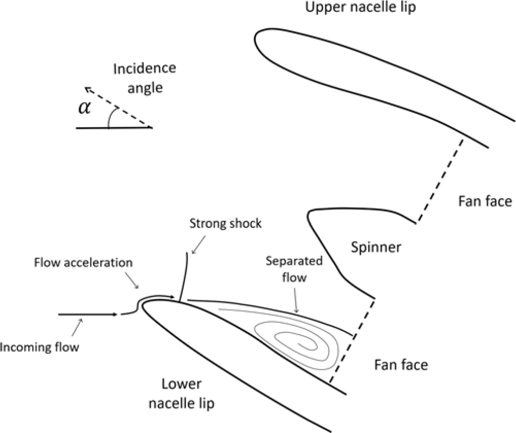
When the freestream flow enters the engine inlet at large angles of attack, the acceleration of this flow around the nacelle lip causes a shock wave to form. This normal shock on the lower nacelle lip causes the boundary layer to thicken, and if the shock is strong enough, shock-induced separation can occur and the intake can become fully (critically) separated. Figure 1 shows the key features of the intake flow behaviour at a high (critically separated) incidence.
Schematic of the flow physics around an intake at a high-incidence, critically separated condition.

Due to the increased bypass ratio of future engines, the diameter of the engine inlets is increasing and therefore, to compensate for this and reduce weight and drag, engine intakes will need to be shorter and thinner. These shorter intakes have steeper diffuser angles, which exacerbates the problem of shock-induced separation at off-design conditions. Oriji and Tucker(Reference Oriji and Tucker2) studied the complex engine inlet flow behaviour at high incidence and in crosswinds, and Hall and Hynes(Reference Hall and Hynes3) investigated the hysteresis phenomena associated with flow separation and reattachment. The impacts of inlet distortion on the stability of the fan(Reference Cao, Vadlamani, Tucker, Smith, Slaby and Sheaf4) and the fanintake interaction on the incidence tolerance(Reference Larkin and Schweiger5,Reference Boldman, Iek, Hwang, Larkin and Schweiger6) have also been studied. These show that the suction of the fan is actually capable of slightly suppressing nacelle separation.
A redesign of short engine intake shapes was carried out by Peters et al.(Reference Peters, Spakovszky, Lord and Rose7). That work focused on the redesign of the entire engine inlet geometry using a spline-based inlet design tool to reduce the likelihood of intake separation. A parametric design study of inlet lengths and diameters was carried out, and it was concluded that the recommended inlet length-to-diameter ratio is between 0.25 and 0.4, otherwise losses in fan efficiency offset gains in propulsive efficiency. Christie et al.(Reference Christie, Heidebrecht and MacManus8) used design variables based on the intuitive class shape transformation (iCST) curves to reshape nacelle inlets. They were able to achieve performance similar to a mature inlet design in a rapid fashion using intuitive design variables. These investigations redesigned the entire inlet profile to find improved designs. Rather than a full redesign of the nacelle inlet, this work assesses the addition of shock control bumps as a method of controlling and preventing shock-induced separation on intake geometries. In this approach, the baseline nacelle geometry remains unaltered apart from the addition of bumps.
1.2 Shock control on aerodynamic surfaces
To combat the adverse effects of shock waves (including shock-induced separation), several methods have been proposed to alleviate shock strength on aerodynamic surfaces. These include synthetic jets(Reference Qin, Zhu and Shaw9), slotting of aerofoil surfaces(Reference Smith, Babinsky, Fulker and Ashill10), porous surfaces(Reference Chokani and Squire11) and shock control bumps(Reference Tai12,Reference John, Qin and Shahpar13) . The aim of these methods, either active (requiring energy input) or passive (geometric modification only), is to reduce the strength of the shock, ideally turning it into isentropic compression waves, and therefore reduce the associated adverse effects. Shock control bumps are adopted in this work for nacelle flow control at high incidences. They are cost effective, as they require a simple modification to the baseline geometry and have a low skin friction drag penalty.
1.3 Shock control bumps
Shock control bumps are bumps added to aerodynamic surfaces to alter the behaviour of the shock and improve aerodynamic performance. A shock bump can be considered as a physics-based surface reprofiling for effective shock control.
The earliest example of shock control bump usage is in the design of the dromedaryfoil in the 1970s(Reference Tai14,Reference Tai, Huson, Hicks and Gregorek15) . This was a modified supercritical aerofoil with a bump added in an attempt to increase its drag divergence Mach number. The ‘hump’ was shown to weaken the shock wave when implemented in the right position. This also demonstrated the importance of shock control bump positioning, because if the bump was misplaced, an increase in wave drag was seen.
Ashill et al.(Reference Ashill and Fulker16) found that a significant reduction in drag could be achieved for a Two-Dimensional (2D) aerofoil by the correct application of a shock control bump, however when the shock position changed, severe drag penalties were incurred due to secondary shocks and separation being produced. Drela and Giles(Reference Drela and Giles17) carried out numerical studies into shock control in 1987, describing the behaviour of shock-induced separation. Sommerer et al.(Reference Sommerer, Lutz and Wagner18) optimised shock control bumps at various Mach numbers. They concluded that the bump height, width and position of the bump peak are the key parameters. Stanewsky et al.(Reference Stanewsky19) concluded that shock control bumps had the greatest potential out of a range of shock control devices tested. In that project(Reference Stanewsky19), a large amount of research was carried out into shock control bumps, with both 2D and Three-Dimensional (3D) analysis, although no optimisation was undertaken.
Qin et al.(Reference Qin, Monet and Shaw20,Reference Qin, Wong and Le Moigne21) first proposed 3D shock control bumps, allowing additional design complexity. They showed that 3D bump configurations can be more robust than 2D bump designs through adjoint-based design optimisation. Collins et al.(Reference Colliss, Babinsky, NÜbler and Lutz22) tested shock control bumps in a wind tunnel, and analysed the performance of shock control bumps at off-design conditions. They noted that, at off-design conditions, even smooth bumps can create vortical flow between the individual bumps and that large, separated regions occur.
1.4 Shock control bump type
Two types of bump are generally favoured in the literature: smooth and ramp-type bumps. Both types of bump consist of a gradually raised surface which compresses the flow, and then a rear part that returns the flow to the datum surface. A description of the different types of bumps is given in(Reference Bruce and Colliss23). Smooth bumps are used in this investigation, as they have been shown to result in less pressure loss than ramp-type bumps, and reducing the total pressure loss produced is a critical concern for intake design.
Smooth bumps (used here) have a smooth transition between the datum surface and the bump geometry; i.e. where the bump meets the datum surface, the gradient is zero. These type of bumps have been produced through a variety of parameterisation methods, including piece-wise cubic curves(Reference Qin, Wong and Le Moigne21), Hicks–Henne curves(Reference Tian, Liu and Li24) or Class-Shape function Transforms (CST)(Reference Zhu and Qin25,Reference Zhu26) . Smooth bumps create isentropic pre-compression waves upstream of the shock that gradually increase the pressure before the shock. As a result of the pre-compression, the shock strength is reduced, leading to a reduction in wave drag and flow separation.
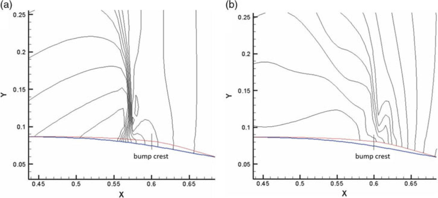
Figure 2 shows an example of how the pre-compression effect works when the bump is optimally positioned. The shock has been delayed and reduced to a series of pre-compression waves, and a ‘knee-like’ structure is formed. This optimised ‘knee-shaped’ flow pattern for shock control bumps was identified(Reference Qin, Wong and Le Moigne21), and has been repeatedly observed in shock control optimisation. The positioning of the bump is crucial. If the bump is placed too far downstream, it can trigger a second shock, while if it is placed too far upstream, it can cause separation. Stanewsky et al.(Reference Stanewsky19) suggested that the peak of the bump should be approximately 5% of the bump length downstream of the original shock location. Qin et al.(Reference Qin, Wong and Le Moigne21) showed that the crest of the bump should be a few percent of chord downstream of the original shock position and that the effectiveness of the bump primarily depends on the bump position and height. A larger height will cause greater pre-compression but may lead to separation downstream of the bump.
The impact of a smooth bump on the shock when positioned in the optimal position: (a) datum geometry static pressure contours and (b) static pressure contours with bump. Image from Qin(Reference Qin, Wong and Le Moigne21).

In this work, the bump geometry can vary in the circumferential direction and is a 3D bump, but the bump is continuous (i.e. the bump height above the datum surface does not necessarily go to zero, as would be the case with multiple 3D bumps with a finite width).
1.5 Aims
Previous work has shown that shock control bumps applied to aerodynamic surfaces have the ability to reduce shock strength and shock-induced separation. The impact of applying shock control bumps to an engine inlet is unknown however. At high incidence, engine inlets can suffer from strong shock-induced separation, which can have a disastrous effect on engine performance. A method of reducing shock strength at high incidence would therefore be beneficial. The aims of this work are to investigate whether the addition of shock control bumps to an engine intake lower lip has the capability to reduce shock strength and shock-induced separation, and to test whether doing this can extend the operating range of the inlet. The bump geometries are optimised to find the most suitable design and maximise the benefit achieved.
This paper is split into two sections. Firstly, detailed analysis of the baseline geometry and its behaviour at high incidence is carried out. Optimisation is then carried out to design bumps that provide a benefit in terms of shock strength, pressure loss and unseparated operating incidence. Finally, the impact of the bumps on the cruise performance of the intake is investigated.
2.0 GEOMETRY, MESHING AND FLOW SIMULATION SET-UP
2.1 Geometry and parameterisation
The geometry under investigation is a high-bypass-ratio engine intake. The external profile is a NACA-1 series aerofoil. The internal profile is a super-elliptic lip with a spline to define the diffuser. The investigations are carried out on an isolated intake geometry, as the inclusion of the fan lies beyond the scope of this project. From previous experience it is understood that, while including the fan in the simulations would affect the angle-of-attack at which separation occurs and the magnitude of distortion(Reference Cao, Vadlamani, Tucker, Smith, Slaby and Sheaf4), a redesign that is beneficial in a nacelle-only simulation will also be beneficial once the fan is included.
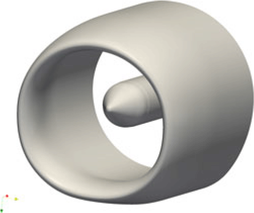
A Computer-Aided Design (CAD) representation of the geometry was converted into a series of 2D constant- $\theta$ (circumferential) slices, which allow meshing and geometry modification by PADRAM(Reference Shahpar and Lapworth27) (a geometry and mesh editor). These 2D slices can be individually perturbed to modify the 3D geometry (which is smoothly interpolated from the 2D sections during the meshing process) and produce smooth bumps. The datum nacelle geometry can be seen in Figure 3.
The datum nacelle and spinner geometry generated in PADRAM(Reference Shahpar and Lapworth27).

2.1.1 Bump creation via the CST method
The Class-Shape Transformation (CST) method(Reference Kulfan28) is used in this work to define the bump geometries. The CST method uses several Bernstein polynomials to create smooth contour bumps. Third-order CST bumps are used. The bumps are defined by a start and end point on the datum surface and the amplitudes for the four polynomials. These amplitudes control the bump height and asymmetry.
The CST method has two parts: the class function and the shape function. The class function determines the order of the geometry, then the shape function is employed to control it. Here, the class parameters N1 and N2 are set to 3. This sets the general class of shapes to follow a shape similar to a cubic spline. The full description of the 2D CST bump is as follows(Reference Hinchliffe29):
 \begin{equation}\epsilon (\phi) = \mathcal{C}_{3.0}^{3.0}(\phi) \space . \space \sum_{i}^{n} A_i \space . \space \mathcal{S}_i(\phi)\end{equation}
where  $\epsilon (\phi)$ is the relative bump height that is added to the datum geometry,
 $\phi$ is the normalised distance between the bump start and end points, C is the class function, n is the b-spline polynomial order (here 3), A is the amplitude of each function and S is the shape function.
The class function is
 \begin{equation}\mathcal{C}_{N_2}^{N_1} (\phi) = \phi^{N_1} \space . \space (1-\phi)^{N_2}.\end{equation}
The shape function is
 \begin{equation}\mathcal{S}_i(\phi)=\sum_{r=0}^{n} K_{r,n} \phi^r (1-\phi)^{n-r},\end{equation}
 \begin{equation}K_{r,n} = \frac{n!}{i!(n-i)!}.\qquad\qquad\end{equation}
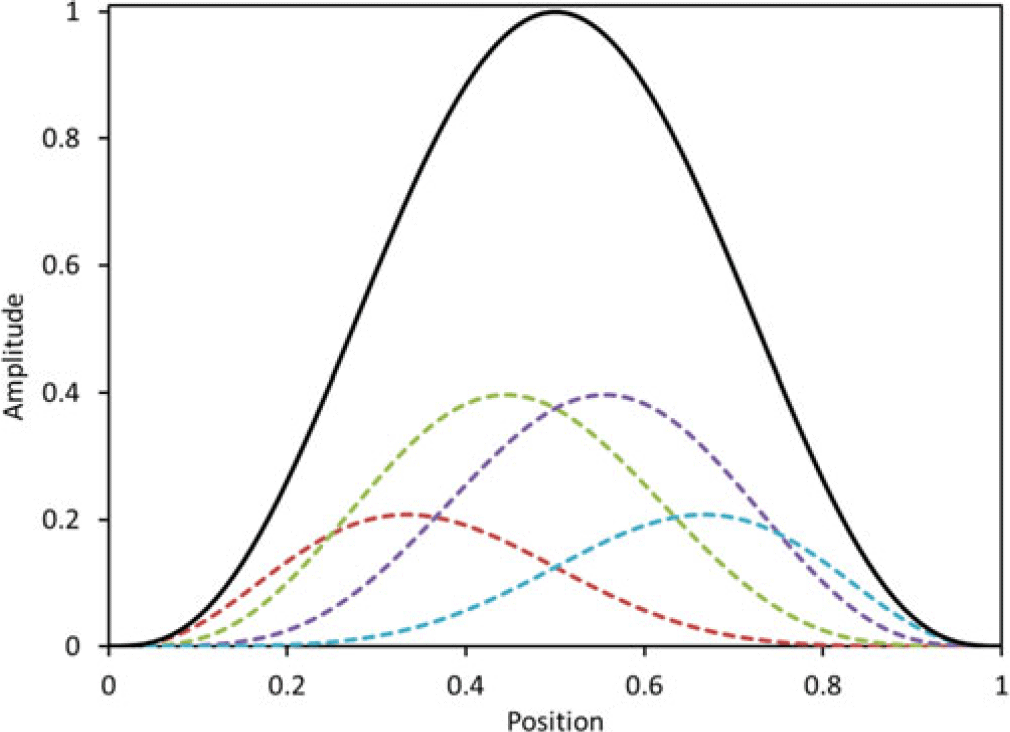
Figure 4 shows how the bump geometry (solid black line) is a sum of the four shape function polynomials (coloured dashed lines). During geometry parameterisation, the bumps are defined by a start and end point on the datum surface, and the amplitudes of the four polynomials which control the overall bump height and asymmetry. The CST bump parameterisation provides a high degree of flexibility, enabling the generation of smooth, asymmetric bumps. For the continuous bumps used in this work, the 2D CST bump profile is specified at several positions in the circumferential direction and this is then smoothly interpolated using a cubic b-spline onto every  $\theta$ section of the geometry.
Example 2D CST bump (solid line) and the four shape function polynomials used to construct it (dashed lines).

Global mesh dependence study.

PADRAM mesh of the intake geometry: (a) front view and (b) zoomed side view on the symmetry plane.

Simulation domain and boundary conditions.

2.2 Simulation set-up
2.2.1 Meshing
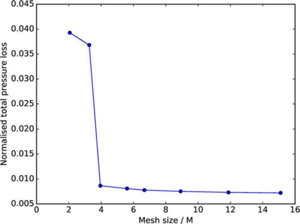
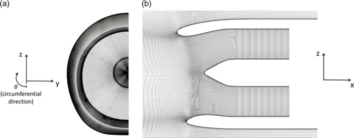
Meshing of the nacelle geometry is carried out in PADRAM(Reference Shahpar and Lapworth27) using the sub-module RApid Meshing for INtakes (RAMIN), making use of a multi-block structural mesh with elliptic smoothing for high quality. A symmetry plane (see Figure 8) is used to reduce computational cost. A mesh dependence study is undertaken to select the appropriate mesh size to be used. The overall mesh size is gradually increased until the change in normalised pressure loss (total pressure loss normalised by the freestream total pressure) measured at the fan face with increasing mesh size is below 1%. This is shown in Figure 5. The jump in values around mesh size of 3M is due to coarser meshes predicting the flow to be critically separated and finer ones not. It was found however during this investigation that the region most sensitive to mesh density was around the shock location, on the upper side of the lower nacelle lip. Even with a globally mesh-independent grid, if too few axial cells are used in the shock region, it is not properly captured, resulting in a false prediction of the flow physics. The mesh in this region was therefore further refined to ensure proper resolution of the shock, even as it moves due to changes in incidence. The first wall cell  $y^+$ is on the order of 1 for the whole nacelle. The mesh in the circumferential direction comprises 130 cells, matching the resolution of the geometry file. The final mesh size is approximately 9M cells. Views of the final mesh used can be seen in Figure 6.
Fan face position and symmetry plane.

2.2.2 The CFD domain
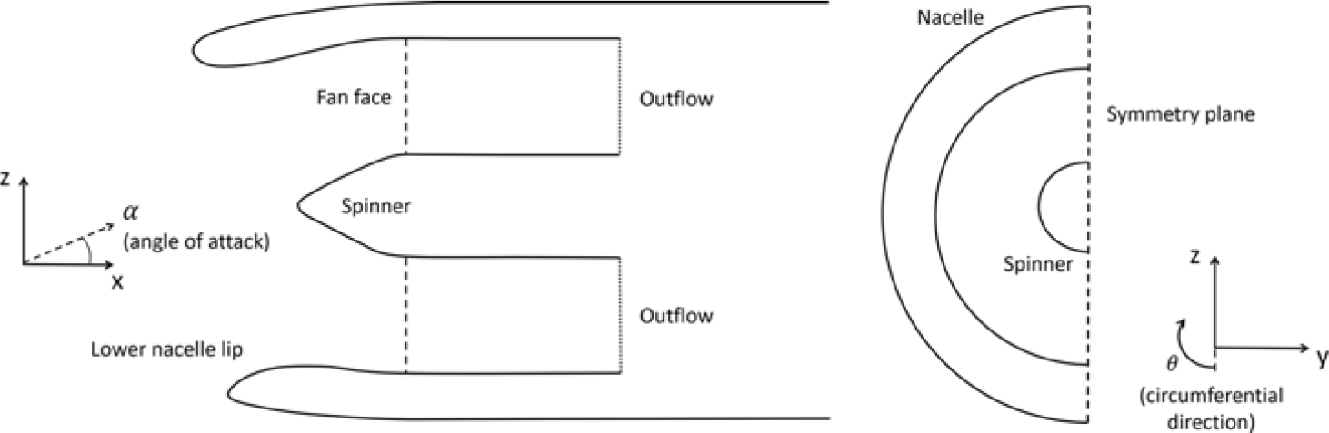
A schematic of the CFD domain can be seen in Figure 7, with more detail in Figure 8. The freestream Mach number is 0.25, and the angle-of-attack ( $\alpha$) is varied throughout the investigations. The freestream total pressure and density correspond to an altitude of 15,000–17,000ft, the limit of the max-takeoff envelope for typical civilian aircraft. The computational outflow boundary condition is located downstream of the fan face, as shown in Figure 8. The fan face is an analysis plane (that does not interact with the flow) positioned where the engine fan would sit. This is used to assess the impact that the intake flow would have on the engine fan. The fan diameter (D) is that for a typical high-bypass-ratio engine for a twin-aisle aircraft. The design is typical of the kind used for 85–115inch fans.
The outflow boundary condition is set by a value of capacity ( $\frac{\dot{m} \sqrt{T_{tot}}}{P_{tot}}$), although the boundary condition is actually specified by the solver using static pressure. The capacity at the exit is calculated from the mixed-out and radially integrated flow properties at each iteration, then the difference between the capacity value and the target is calculated and used to adjust the static pressure value. The capacity outflow is used to provide a fair comparison between different angles of attack or designs. If a fixed mass flow were used, this may draw extra flow through the intake than would occur in reality, where the fan exerts a constant suction on the incoming flow and the mass flow achieved depends on the pressure loss over the intake lip. The capacity was set to a value of 0.0803kg/s/
 $\sqrt{\mathrm{K}}/Pa$. This condition is known to be close to the separation boundary of the lip from previous work and results in a mass flow through the engine of a few hundred kg/s. The nacelle walls have no-slip boundary conditions applied. Because the nacelle geometry is symmetrical, a symmetry plane is used and only half of the geometry is simulated to reduce the computational cost.
2.2.3 CFD solver and governing equations
The finite-volume CFD solver HYDRA(Reference Lapworth30) is used to solve the 3D RANS equations. Here, an overview of the main constitutive equations and the discretisation methods used is given. The Navier–Stokes equations are expressed as
 \begin{equation}\frac{\partial Q}{\partial t} + \frac{\partial F_{x}}{\partial x} + \frac{\partial F_{y}}{\partial y} + \frac{\partial F_{z}}{\partial z} = 0,\end{equation}
where
 \begin{equation}Q = \left(\begin{array}{c}\rho\\ \rho u\\ \rho v\\ \rho w\\ \rho E\end{array}\right), \quad F_{x} = \left(\begin{array}{c}\rho u\\ \rho u^{2}+p-\tau_{xx}\\ \rho uv - \tau_{yx}\\ \rho uw - \tau_{zx}\\ (\rho E +p)u - u\tau_{xx} - v\tau_{yx} - w\tau_{zx} + q_{x}\end{array}\right)\end{equation}
Q are the quantities that vary over time in the control volume, and F are the fluxes that enter or leave the control volume. The heat flux is given by  $q_{x}=-k\frac{\partial T}{\partial x}$. Expressions for
 $F_y$ and
 $F_z$ follow that for
 $F_x$ and can be found in(Reference Moinier31).
 $\rho$, u, v, w, p and E denote the density, the three Cartesian velocity components, the static pressure and the total internal energy, respectively. The equation of state for an ideal gas is required to complete the equations. The coefficient of thermal conductivity is
 $k=\frac{\gamma \mu}{\rm Pr}$, and
 $\rm Pr$ is the Prandtl number (
 $\rm Pr$ = 0.72 for air). The shear stresses are given by
 \begin{equation}\tau _{xx}=2\mu \frac{\partial{u}}{\partial{x}}+\lambda\left(\frac{\partial{u}}{\partial{x}} + \frac{\partial{v}}{\partial{y}} + \frac{\partial{w}}{\partial{z}} \right)\end{equation}
 \begin{equation}\tau _{yy}=2\mu \frac{\partial{v}}{\partial{y}}+\lambda\left(\frac{\partial{u}}{\partial{x}} + \frac{\partial{v}}{\partial{y}} + \frac{\partial{w}}{\partial{z}} \right)\end{equation}
 \begin{equation}\tau _{zz}=2\mu \frac{\partial{w}}{\partial{z}}+\lambda\left(\frac{\partial{u}}{\partial{x}} + \frac{\partial{v}}{\partial{y}} + \frac{\partial{w}}{\partial{z}} \right)\end{equation}
 \begin{equation}\tau _{xy}=\tau _{yx}=\mu \left(\frac{\partial{u}}{\partial{y}} + \frac{\partial{v}}{\partial{x}} \right), \quad \tau _{xz}=\tau _{zx}=\mu \left(\frac{\partial{u}}{\partial{z}} + \frac{\partial{w}}{\partial{x}} \right), \quad \tau _{yz}=\tau _{zy}=\mu \left(\frac{\partial{v}}{\partial{z}} + \frac{\partial{w}}{\partial{y}} \right),\end{equation}
where the molecular viscosity is modelled by Sutherland’s law,
 \begin{equation}\mu=\frac{1.461 \times 10^{-6}T^{3/2}} {T+110.3},\end{equation}
and the bulk viscosity  $\lambda$ is defined via the Stokes hypothesis(Reference Stokes32):
 \begin{equation}\lambda = -\frac{2}{3}\mu\end{equation}
The Spalart–Allmaras turbulence model(Reference Spalart and Allmaras33) is used to close the steady RANS equations. HYDRA is an unstructured solver that uses an edge-based data structure with the flow data stored at the cell vertices. A flux-differencing algorithm based on a Jameson–Schmidt–Turkel (JST) with matrix dissipation scheme is used for the space discretisation. For the steady-state solution, a five-stage Runge–Kutta scheme is used. An element-collapsing multi-grid algorithm accelerates the convergence to steady state. Further details on the calculation of the inviscid fluxes, the viscous fluxes and convergence can be found in(Reference Moinier31). Validation of HYDRA can be found in(Reference John, Qin and Shahpar13).
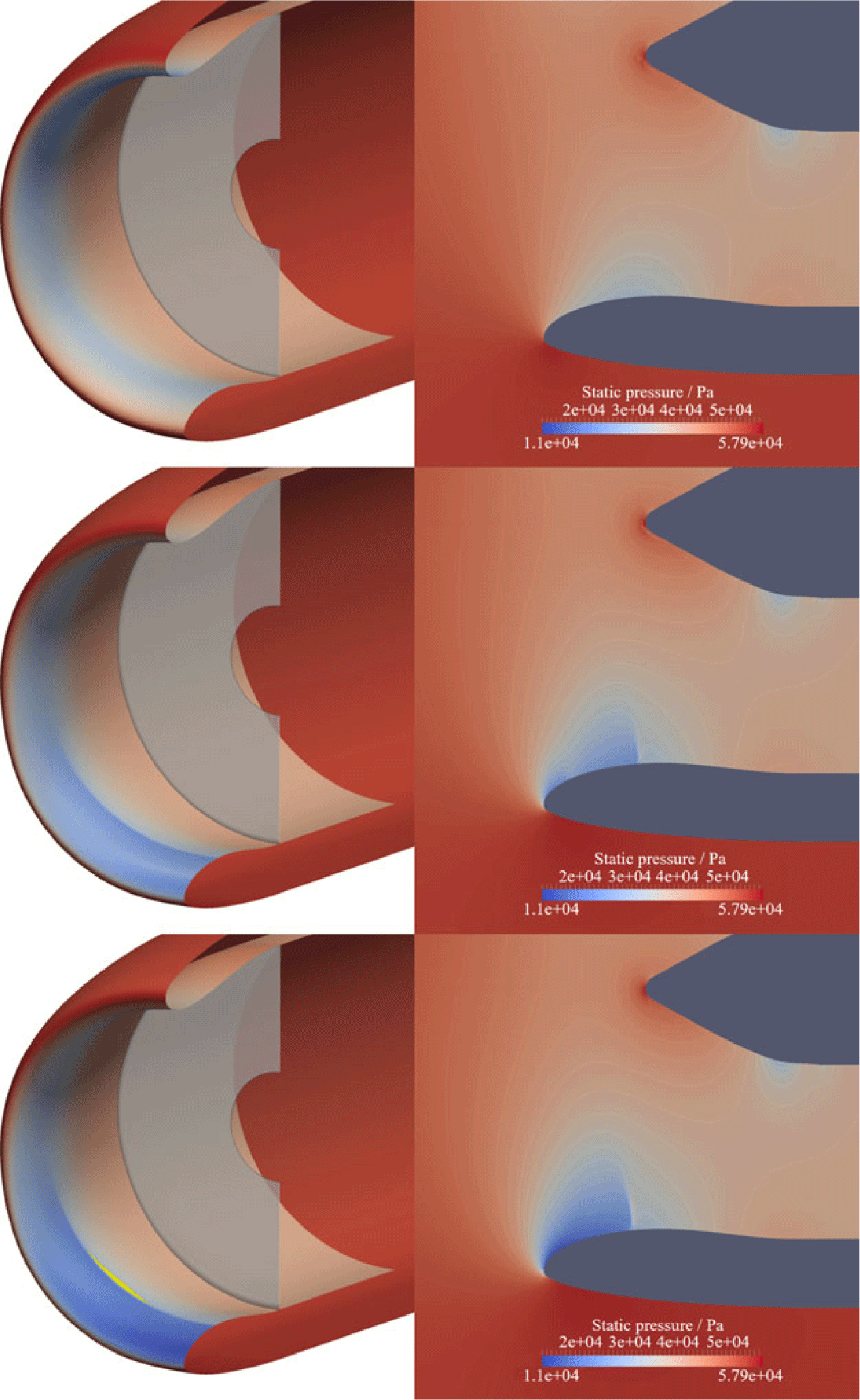
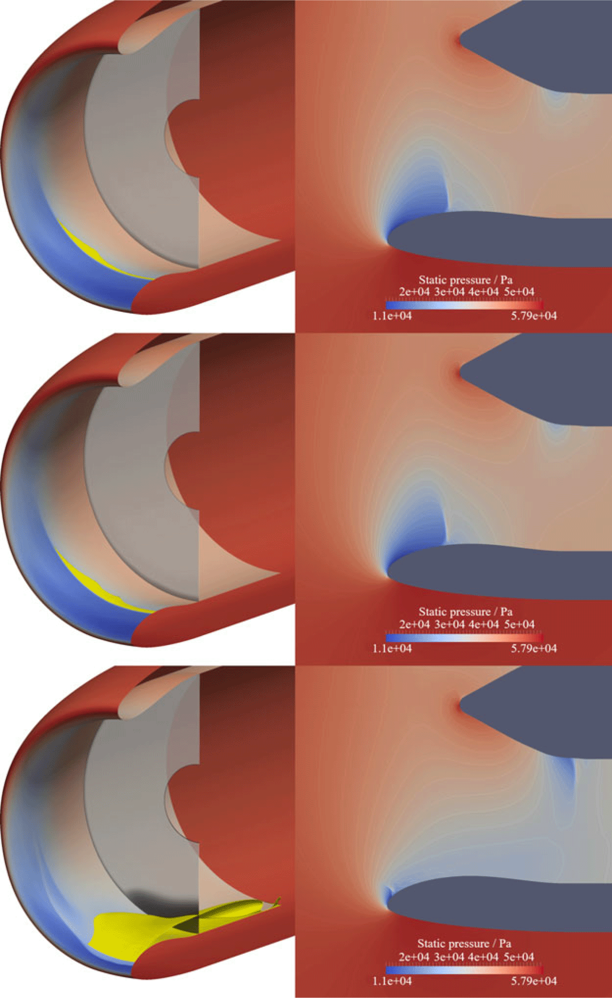
Flow behaviour and separation (yellow) at  $\alpha$ = 0
 $^\circ$ (top), normal take-off (NTO) (middle) and
 $\alpha_{\textit{crit}}$-3
 $^\circ$ (bottom).

Flow behaviour and separation (yellow) at  $\alpha_{\textit{crit}}$−1
 $^\circ$ (top),
 $\alpha_{\textit{crit}}$ (middle) and
 $\alpha_{\textit{crit}}$+1
 $^\circ$ (bottom).

3.0 ANALYSIS OF THE BASELINE GEOMETRY
To analyse the flow features of the datum geometry, the nacelle is simulated at a range of angles of attack to identify the operating limits of the nacelle. To understand the impact of the flow through the intake on engine performance, it is necessary to assess its impact on the fan. To do this, analysis of the flow at the fan face position is carried out. Figure 8 shows the location of the fan face in the simulation domain, as well as details of the geometry set-up.
3.1 Variation of flow features with incidence
Figures 9 and 10 show the flow features of the nacelle as the angle-of-attack is varied from  $\alpha$ = 0
 $^\circ$ to
 $\alpha_{\textit{crit}}$+1
 $^\circ$ (where
 $\alpha_{\textit{crit}}$ is the angle beyond which the datum geometry becomes critically separated). The normal take-off angle is the effective incidence experienced by the engine during take-off. This will depend on the high-lift configuration of the wing and is typically between 15
 $^\circ$ and 20
 $^\circ$. The spinner is not shown in the 3D images for clarity. It can be seen how at higher incidence the flow accelerates over the lower nacelle lip and forms a low-pressure region. Static pressure contours show the shock formation and how it strengthens as the incidence angle is increased. The shock-induced separation is highlighted by 3D iso-surfaces of zero axial velocity (in yellow). It can be seen that this separated region begins off-centre; the reason for this is described in Section 3.6.
The impact of this separation on the fan is shown via the contour of entropy at the fan face (where dark regions indicate high entropy) in Figures 9 and 10. Increased entropy is a result of viscous effects in the boundary layer and the shock once it forms. An increase in entropy at the fan face indicates an increase in pressure loss and blockage, which would adversely affect the engine’s operating performance. A small separation bubble begins to appear at  $\alpha_{\textit{crit}}$-3
 $^\circ$, and gradually increases in size as the shock strength increases. At
 $\alpha_{\textit{crit}}$+1
 $^\circ$, the flow can no longer remain attached and a sudden increase in the amount of separation and entropy at the fan face is seen.
3.2 Variation in pressure loss and mass flow with incidence
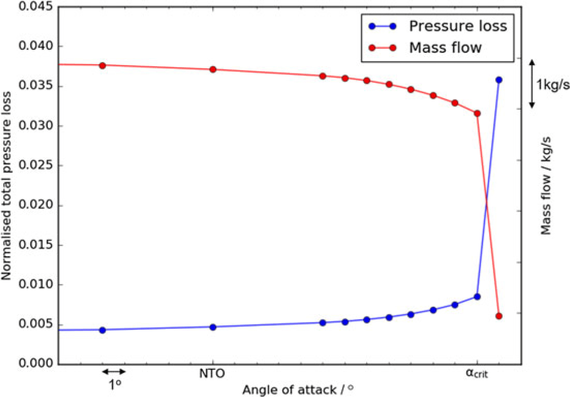
Figure 11 shows the variation in pressure loss (total pressure loss normalised by the freestream total pressure) and mass flow at the fan face for various angles of attack. These can be used to indicate how favourable the flow entering the fan is. Greater pressure loss is caused by boundary layer thickening, flow separation and increased shock strength. Due to the capacity boundary condition imposed at the engine outflow, increased pressure loss results in lower mass flow. A steady increase in pressure loss (and reduction in mass flow passing through the fan face) can be seen as the angle is increased (due to greater shock strength and separation) up until  $\alpha_{\textit{crit}}$. This is the incidence beyond which the intake becomes critically separatedFootnote 1. At
 $\alpha_{\textit{crit}}$+1
 $^\circ$, a sudden rise in pressure loss and drop in mass flow is seen. This is the critical point that must be avoided during engine operation, as the large disturbance to the fan would severely decrease performance and could even stall the fan. Hence the operating range for this intake is
 $\alpha_{\textit{crit}}$ and less.
Variation in normalised total pressure loss and mass flow at the fan face with angle-of-attack, showing that the operating range for the datum nacelle is  $\alpha \leq \alpha_{\textit{crit}}$.

3.3 Experimental validation
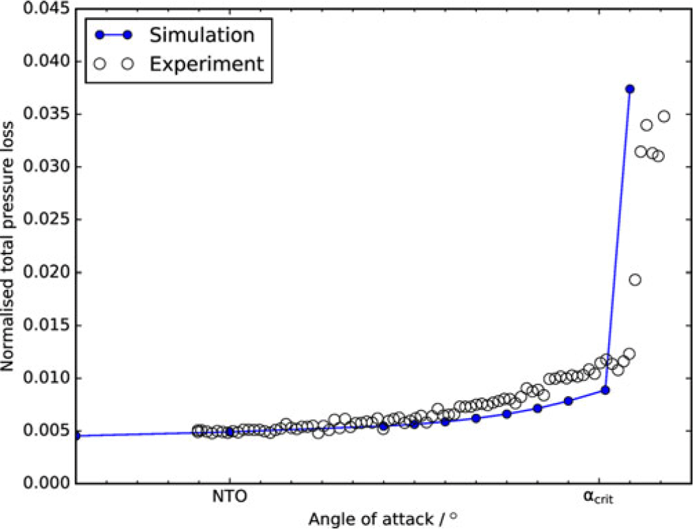
Experimental validation is shown in Figure 12. It can be seen that the pressure loss increase with incidence is well captured. The critical incidence is quite closely reproduced in the simulation compared with the experiment, as is the magnitude of the pressure loss after the separation point. This gives confidence in the simulation’s ability to predict the physics.
Validation against experimental data.

3.4 Shock-induced separation
Shock-induced separation is the process by which the severe adverse pressure gradient across the shock causes the boundary layer to separate. As can be seen in Figure 10, some shock-induced separation occurs from  $\alpha_{\textit{crit}}$-3
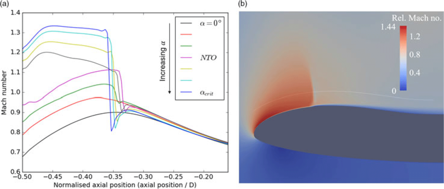
 $^\circ$ (indicated by the yellow iso-contour of zero axial velocity, which demonstrates a region of reverse flow). The process of this shock-induced separation can be seen in Figure 13b. This shows the Mach number along a slice at circumferential position
 $\theta$ = 10
 $^\circ$ for
 $\alpha_{\textit{crit}}$−1
 $^\circ$. The circumferential direction is measured clockwise from bottom dead centre (
 $\theta$ = 0
 $^\circ$) as shown in Figure 8. The process of the shock terminating at the nacelle surface, interacting with the boundary layer and triggering separation, can be seen. The sudden increase in boundary-layer thickness (and separation) can be seen by the low-velocity region after the shock impingement point.
(a) Mach number profiles at bottom dead centre for various incidences along the constant wall-distance line shown in (b).

3.5 Shock variation with incidence
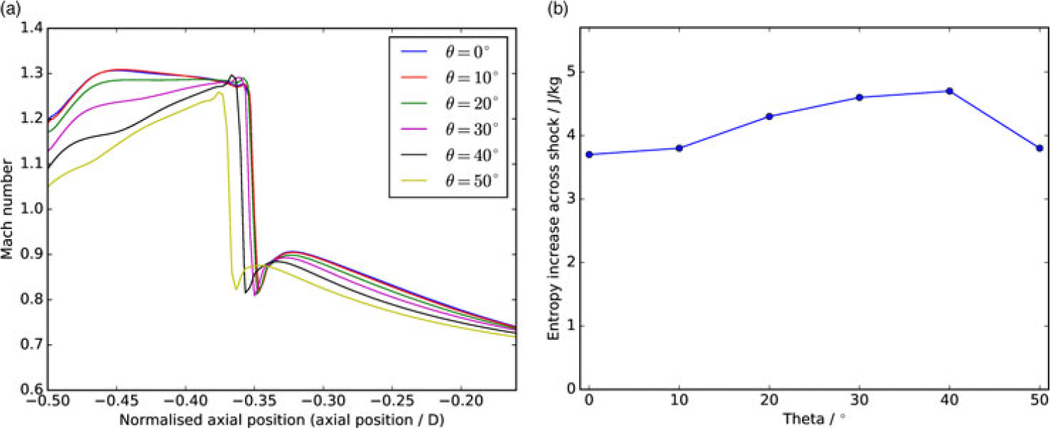
To further understand how the shock behaviour varies with incidence, the shock strength (drop in Mach number across the shock along a streamline) a small distance away from the wall is analysed. This gives a clearer picture of the shock behaviour. Figure 13 shows how the shock at  $\theta$ = 0
 $^\circ$ varies with incidence. This is plotted using Mach number, measured at 0.1m from the wall (along the white line shown in Figure 13b). The axial position is relative to the fan face, and normalised by the fan diameter. It can be seen how the shock forms and its strength increases steadily with increasing angle-of-attack. The pre-shock Mach number increases with
 $\alpha$, as greater acceleration of the flow around the nacelle lip increases its velocity. The post-shock Mach numbers are reduced to subsonic speeds with a small range between different incidences as expected from normal shock theory.
3.6 Flow variation in the circumferential direction
As can be seen in Figure 10, the amount of shock-induced separation at high angles of attack varies in the circumferential direction. Separated flow is also isolated to between  $\theta$ = 0
 $^\circ$ (bottom dead centre) and
 $\theta$ = 45
 $^\circ$. This demonstrates that there is a variation in the flow behaviour occurring in the circumferential direction, resulting in a variation in shock strength with
 $\theta$. Here, further analysis of the flow is carried out at
 $\alpha_{\textit{crit}}$−1
 $^\circ$. Figure 14a shows the shock profiles at
 $\theta$ positions from 0
 $^\circ$ to 50
 $^\circ$, and it can be seen that the pre-shock flow varies with
 $\theta$. The shock strength is difficult to judge from this figure however, so an alternative approach is needed.
Shock variation with theta at  $\alpha_{\textit{crit}}$−1
 $^\circ$: (a) Mach number profiles, and (b) shock strength variation in theta measured by entropy increase along a streamline across the shock.

The entropy increase from before to after the shock (along a flow streamline) gives a direct measure of the shock strength. For these results, the entropy jump across the shock at 0.1m distance from the wall is measured for each  $\theta$ angle at
 $\alpha_{\textit{crit}}$−1
 $^\circ$. The variation in shock strength with
 $\theta$ can be seen in Figure 14b. This shows that the strongest shock is around
 $\theta$ = 30–40
 $^\circ$, which reflects the regions of highest separation seen in the top image in Figure 10.
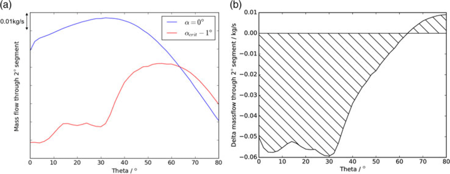
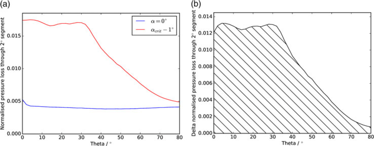
As suggested by the above results, the pressure loss, and therefore mass flow, at the fan face is not evenly distributed with  $\theta$. To understand the circumferential distribution of these flow features, analysis can be carried out at the fan face. The flow properties are integrated (using area averaging) over 2
 $^\circ$ sectors to give the circumferential distributions shown in Figure 15. Figure 15 shows the variation in mass flow with
 $\theta$ at the fan face. The delta between zero and
 $\alpha_{\textit{crit}}$−1
 $^\circ$ (subtraction of the mass flow values at
 $0^\circ$ from values at
 $\alpha_{\textit{crit}}$−1
 $^\circ$) shows how the mass flow is reduced by the increased angle-of-attack and the associated losses. It can also be seen that a slight increase in mass flow occurs above
 $\theta$ = 60
 $^\circ$, as the flow is redistributed due to the blockage near to bottom dead centre. The drop in mass flow, seen for the majority of the nacelle, is due to the increased pressure loss caused by shock and separation at increased incidence. The normalised pressure loss (total pressure loss normalised by the freestream total pressure) distribution therefore reflects the mass flow distribution (shown in Figure 16 and later in Figure 25b). The normalised total pressure loss was calculated by area-averaging the total pressure over each
 $2^\circ$ sector, subtracting this value from the total pressure in the far field and then dividing by the total pressure in the far field.
(a) Mass flow versus  $\theta$ at
 $\alpha$ = 0
 $^\circ$ and
 $\alpha_{\textit{crit}}$−1
 $^\circ$, (b) delta mass flow versus
 $\theta$ from
 $\alpha$ = 0
 $^\circ$ to
 $\alpha_{\textit{crit}}$−1
 $^\circ$.

(a) Normalised total pressure loss versus  $\theta$ at
 $\alpha$ = 0
 $^\circ$ and
 $\alpha_{\textit{crit}}$−1
 $^\circ$, (b) delta total pressure loss versus
 $\theta$ from
 $\alpha$ = 0
 $^\circ$ to
 $\alpha_{\textit{crit}}$−1
 $^\circ$.

3.7 Explanation of the most sensitive region in theta
As shown above in Section 3.6, the shock strength and separation are greatest around  $\theta$ = 30
 $^\circ$, and not at
 $\theta$ = 0
 $^\circ$, where one might expect the strongest shock to be, due to the greatest vertical component of the velocity being at this point. The reason for this is due to the geometrical features of this particular nacelle design with 3D shaping in the lower quadrant. As one traverses in the circumferential direction around the nacelle, the local incidence normal to the lip due to the global angle-of-attack reduces as
 $\theta$ increases. This local incidence is maximum at
 $\theta$ = 0
 $^\circ$ and zero at
 $\theta$ = 90
 $^\circ$. This suggests that the acceleration around the lip, and shock strength, will be strongest at lower values of
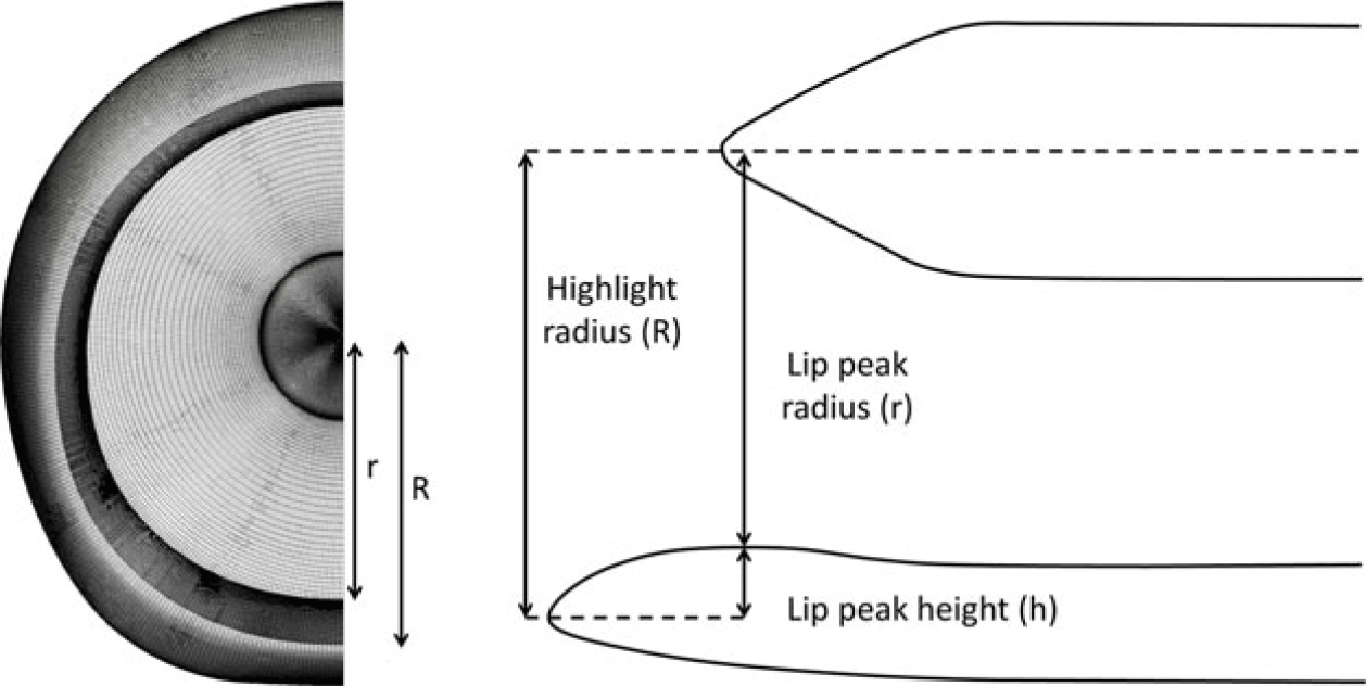
 $\theta$. The nacelle geometry also varies in the circumferential direction, however. Figure 17 shows the front view of the geometry and a diagram that explains the contraction ratio.
Front view of the nacelle geometry (left) and a schematic defining geometric parameters of the nacelle (right).

The Contraction Ratio (CR) is defined as  $CR = \frac{R^2}{r^2}$, where R is the highlight radius and r is the lip peak radius, as shown in Figure 17. For nacelle designs, the contraction ratio reduces as
 $\theta$ increases, as a higher contraction ratio (thicker lip) is more favourable near to bottom dead centre, but a lower contraction ratio (thinner lip) is preferred near to
 $\theta$ = 90
 $^\circ$ due to crosswind considerations. For this particular nacelle, constraints on the nacelle internal volume mean that it is ‘flat-bottomed’, so the component of
 $\alpha$ remains quite large until higher values of
 $\theta$ than if the nacelle geometry were circular. The acceleration around the nacelle lip and the shock strength are related to the local incidence and the contraction ratio. For this geometry, there is a point in the circumferential direction where the combination of local incidence and the contraction ratio results in a stronger acceleration than at bottom dead centre (
 $\theta$ = 0
 $^\circ$), which pushes the strongest shock and greatest separation further around the nacelle away from bottom dead centre, as described above.
4.0 OPTIMISATION OF SHOCK CONTROL BUMPS
To assess the impact of adding shock control bumps to the nacelle surface, their effect is tested at  $\alpha_{\textit{crit}}$−1
 $^\circ$. This operating condition is chosen to be close to the full-separation incidence but not quite at the limit of critical separation (as shown in the analysis in Section 3). The approach of this optimisation is to reduce the separation and pressure loss at a single point, and to then assess whether improving the flow behaviour at this point near to critical separation allows the nacelle to operate without separation at higher incidences. To assess any improvement through the use of bumps, the mass flow and pressure loss are measured at the fan face. An increase in mass flow, or reduction in pressure loss, indicates a more favourable design.
4.1 Shock control bump positioning
Based on the experience of previous shock bump optimisation, the initial placement of the bumps is set so that 60% of the bump is downstream of the datum shock position. This follows the recommendation by Qin et al.(Reference Qin, Wong and Le Moigne21) and Hinchliffe and Qin(Reference Hinchliffe and Qin34). The bumps are positioned from 0 $^\circ$ to 60
 $^\circ$
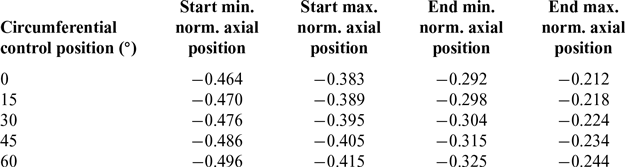
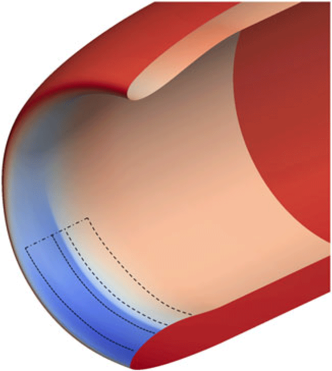
 $\theta$, as this is the region where separation mostly occurs and the region where increased angle-of-attack is most detrimental to the flow (see Figure 16b). The axial start and end positions of the bump are allowed to vary. This offers flexibility in the bump geometry and greater potential to find a design that performs well across the range of circumferential positions. Figure 18 and Table 1 show the permitted variation in bump start and end positions.
The parameter ranges for the varying start/end point optimisation. The normalised axial positions (axial position /D) are given relative to the fan face

The bump start (dots) and end (dashes) position regions.

4.2 Optimisation set-up
4.2.1 Bump design variables
For the optimisation of the bumps, the bump height is controlled at five  $\theta$ positions, in the region shown in Figure 18. The geometry is smoothly interpolated in the circumferential direction using a cubic spline. The bump start and end positions and the four CST parameters are allowed to vary for each of the five bump control positions, thus resulting in 30 parameters.
4.2.2 Objective function
The objective for the optimisation is to maximise the mass flow through the fan face (an increase in mass flow indicates a reduction in pressure loss across the nacelle), but as the optimiser must minimise positive functions, the objective function is set to the mass flow for the design being assessed subtracted from a value slightly higher than the datum mass flow at zero incidence. Thus, if the mass flow for the design is larger, the objective function reduces and the optimiser recognises this as a beneficial design. For some of the designs large separation can occur and the convergence of the simulation becomes poor during the optimisation. Hence, when calculating the objective function, the last few hundred iterations of each simulation are averaged.
4.2.3 Optimiser
The optimisation method used for this work is the Multi-point Approximation Method (MAM) developed by Polynkine et al.(Reference Polynkine, Van Keulen and Toropov35) MAM is a gradient-based method that uses localised Design of Experiments (DoE) and dynamic trust regions to efficiently search through the design space. When using MAM, an initial generation of simulations (chosen by DoE) is carried out around the start point. A response surface is constructed for this region, and the sub-optimal point found. The search is then moved to this point, where a new generation is constructed and the process is repeated until the search converges on the optimal design. The MAM has been shown to be an efficient and consistent approach for a wide range of large industrial optimisation problems. Examples of its usage can be found in(Reference John, Qin and Shahpar13, Reference John, Shahpar and Qin36).
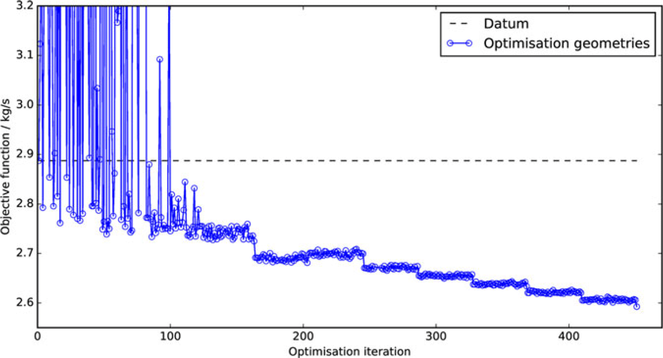
The convergence history of the optimisation is shown in Figure 19. It can be seen that the first couple of optimisation generations include designs that under-perform compared with datum, but MAM moves the search away from this region and the success of future MAM generations can be seen.
Optimisation convergence.

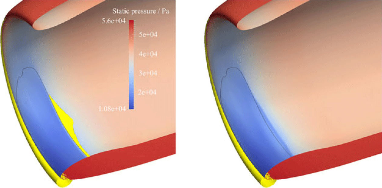
The effect of this optimised geometry on the flow is shown in Figure 20. It can be seen how the optimised design completely eliminates the separation and delays the shock position along the region where the bump is placed. Table 2 gives a performance comparison with the datum design of this optimised geometry. It can be seen that the optimised design results in a significant reduction in delta normalised total pressure loss compared with the datum geometry.
Comparison of the optimised bump with datum

Shock position and separation (yellow) for the datum (left) and optimised (right) geometries. The datum shock position is indicated by the black line.

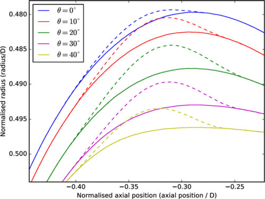
The optimised geometry is compared with the datum geometry in Figure 21. It can be seen how the optimised design’s bump geometry varies circumferentially. The bump shape, overall amplitude and start/end positions all vary, which is key to the benefit of the design. The next section describes the impact of the optimised geometry on the flow at the condition at which it was designed. The performance of the optimised design at a wider range of incidence angles is given later in Subsection 4.4.
Constant-theta geometry contours of the datum (solid) and optimised (dashed) bump geometries. The axial positions are relative to the fan face.

4.3 Further analysis of the optimised design
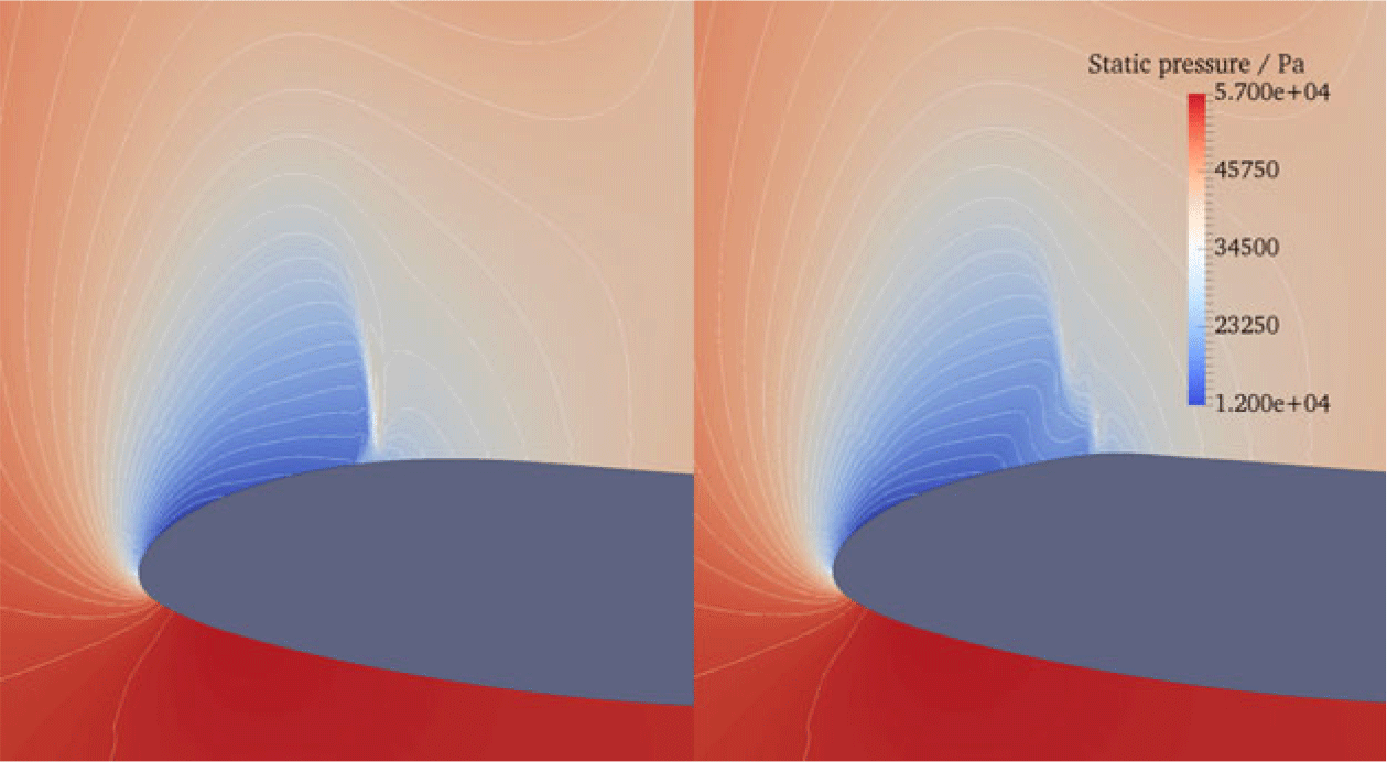
To understand where the benefit of the optimised design comes from, detailed analyses of the impact of the bumps on the flow are carried out in this section. The above results show the benefit achieved through delaying the shock and reducing separation and pressure loss. To demonstrate how the bumps delay the shock and reduce its strength, the pressure contours on a constant- $\theta$ slice near to bottom dead centre for the datum and optimised geometries are compared (see Figure 22). The pre-compression upstream of the shock and the knee-shaped structure formed (reminiscent of that seen in Figure 2 and identified(Reference Qin, Wong and Le Moigne21)) can be seen. The pressure contours are spread out, reducing the pressure/velocity gradient across the shock.
Static pressure contours for the datum (left) and optimised geometry (right) at  $\theta = $ 20
 $^\circ$.

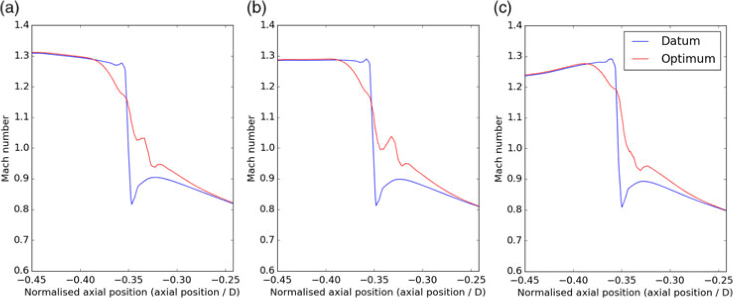
Mach number profiles across the shock at 0.1m wall distance at  $\theta = $ (a) 10
 $^\circ$, (b) 20
 $^\circ$ and (c) 30
 $^\circ$ for the optimised design.

Mach number plots (see Figure 23) measured along a line 0.1m from the wall (shown in Figure 13a) show the change in the shock structure caused by the bumps at various circumferential positions. It can be seen how the shock is weakened by the presence of the bump. The pre-compression effect gradually reduces the Mach number upstream of the shock. The magnitude of the jump in velocity/pressure across the shock is significantly reduced for the optimised design.
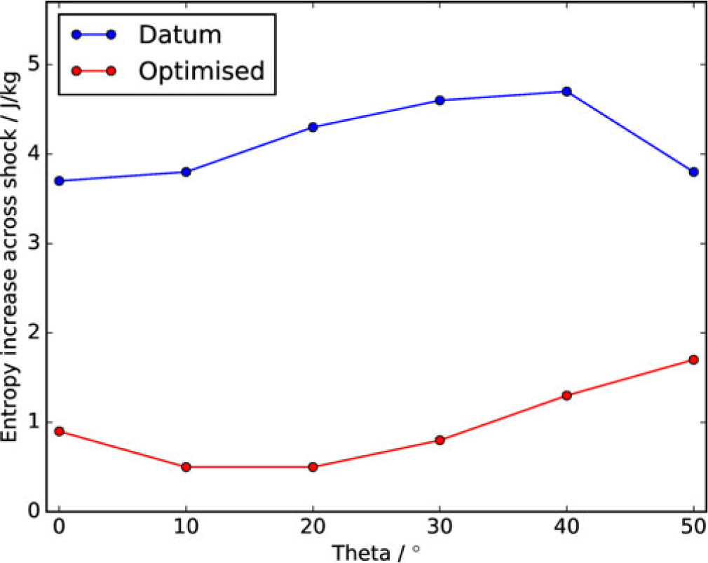
To clearly assess the reduction in shock strength, the entropy change across the shock along a flow streamline (as shown previously in Figure 14b) can be used. This is given in Figure 24 for various  $\theta$ positions. It can be seen that the shock strength is significantly weakened by up to 90%. At
 $\theta\,{=}\,$50
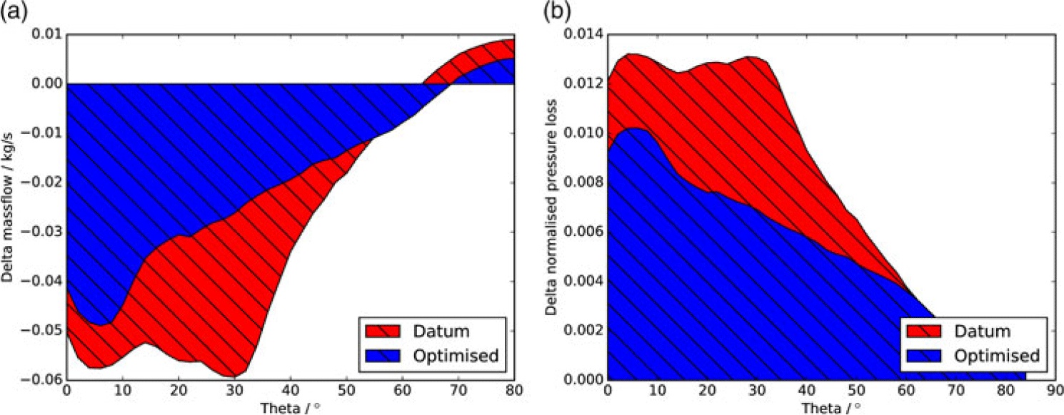
 $^\circ$ the benefit is reduced, as the design begins blending into the datum geometry. Figure 25 shows the circumferential distributions of delta normalised pressure loss and mass flow to the datum geometry at
 $\theta\,{=}\,$0
 $^\circ$. The benefit of the optimum design is clearly seen, with the most significant benefit around
 $\theta\,{=}\,$30–40
 $^\circ$.
Entropy increase across the shock for the datum and optimised geometries.

The (a) mass flow and (b) normalised pressure loss distributions (delta to datum at  $\alpha$ = 0
 $^\circ$) with
 $\theta$ for the datum and optimised geometries.

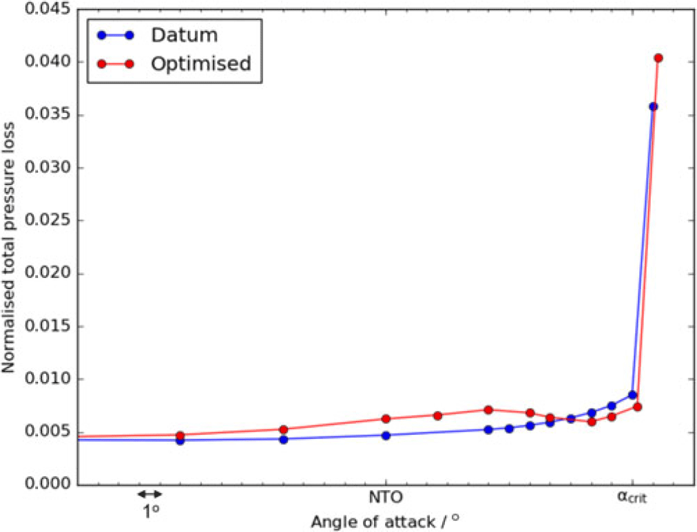
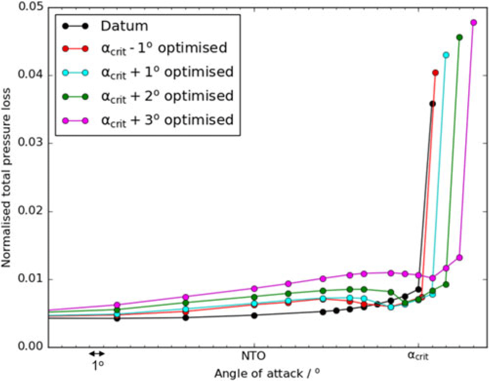
Variation in normalised total pressure loss at the fan face with angle-of-attack for the datum and optimised geometries.

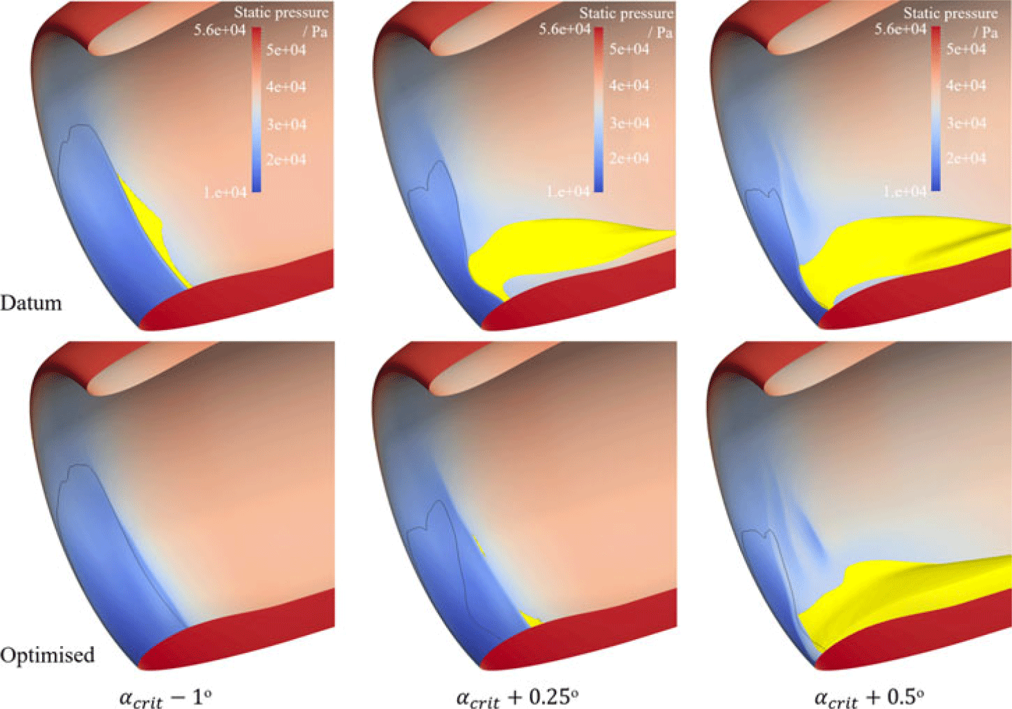
Variation in separation (in yellow) and shock position for the datum and optimised geometries near to the critically separated angle-of-attack.

4.4 Performance at various angles of attack
The two primary objectives of this work are to assess whether bumps can be used to weaken the shock and reduce separation at a non-critically-separated angle-of-attack, and then to see whether this design can be used to extend the maximum angle-of-attack before critical separation of the intake occurs. From here the incidence beyond which critical separation occurs is referred to as the critical incidence of the nacelle. The first of these objectives is clearly achieved above through the optimised design.
The next step is to assess whether this optimised geometry, which can weaken the shock and reduce separation at  $\alpha_{\textit{crit}}$−1
 $^\circ$, is capable of increasing the angle of incidence without critical separation that the nacelle can achieve. To investigate this, the optimised geometry is run at a range of incidences. The resulting normalised total pressure loss at various angles of attack for the optimised and datum geometries are shown in Figure 26.
It can be seen that, as well as increasing the mass flow and reducing the entropy generated at the design condition, the optimised design also increases the operating range of the nacelle slightly, by  $0.25^\circ$. At lower angles of attack, the optimised design performs worse than the datum, albeit generating greater pressure loss. This is due to the bump placement being misaligned with the shock at these incidence angles, possibly increasing the shock strength or leading to regions of separation. The addition of the bump also slightly reduces the through-flow area, resulting in greater losses. At zero incidence (
 $\alpha = 0^\circ$) the pressure loss increase is around 3%.
This drop in performance towards lower angles of attack shows that a multi-point optimisation may be beneficial to improve the design. However, the main objective of this work is to increase the operating range of the engine. Increasing the operating range could lead to an intake redesign where a more aggressive (shorter) inlet is used that uses shock bumps to achieve the same operating range, reducing the overall drag and counteracting the small increase in loss at lower incidence shown here.
Figure 27 shows how the optimised design reduces the separation at  $\alpha_{\textit{crit}}$−1
 $^\circ$ and extends the non-critically-separated range of the intake (increasing the critical incidence) to
 $\alpha_{\textit{crit}}$+0.25
 $^\circ$. This improvement in operating range of
 $0.25^\circ$ is unsatisfactory however, as it does not provide significant benefit. The next section describes optimisations carried out at higher incidence angles to improve upon this benefit.
The performance history for the  $\alpha_{\textit{crit}}$+3
 $^\circ$ optimisation.

5.0 DESIGNING BUMPS TO INCREASE NACELLE OPERATING RANGE
It is demonstrated above that designing the bump at a non-critically-separated angle-of-attack ( $\alpha_{\textit{crit}}$−1
 $^\circ$) only marginally increases the critical incidence of the nacelle. This is likely due to the bump geometry not being correctly aligned with the shock position once the incidence is increased to a critically separated angle (i.e.
 $\alpha > \alpha_{\textit{crit}}$). It is therefore necessary to optimise the bump at a critically separated condition (i.e. to optimise at
 $\alpha > \alpha_{\textit{crit}}$), the issue being that the datum and some of the optimisation geometries tested will be critically separated. When this critical separation occurs, there may be little difference between the objective functions of each bump design, making it difficult for the optimiser to recognise beneficial designs and converge. This was the reason that the approach of optimising at a non-critically-separated angle of incidence was initially adopted. Despite the difficulties of this approach, significant success was achieved as described below.
5.1 Optimising at $\boldsymbol\alpha \boldsymbol > \boldsymbol\alpha_{\textbf{\textit{crit}}}$

Optimisations similar to those used for the optimisation at  $\alpha_{\textit{crit}}$−1
 $^\circ$ are carried out at
 $\alpha_{\textit{crit}}+1^\circ$,
 $\alpha_{\textit{crit}}$+2
 $^\circ$ and
 $\alpha_{\textit{crit}}$+3
 $^\circ$. The seed point of the optimisations (i.e. the initial design that MAM begins its search from) was initially the datum nacelle geometry with no bump, however the optimisations struggled to converge. The
 $\alpha_{\textit{crit}}$−1
 $^\circ$ optimised design is thus used as the seed point of the optimisations. This moves the initial search of the optimisation to designs that are related to the
 $\alpha_{\textit{crit}}$−1
 $^\circ$ optimised design and allows the optimiser to focus on more promising designs. The
 $\alpha_{\textit{crit}}$−1
 $^\circ$ optimised design is critically separated at
 $\alpha_{\textit{crit}}$+1
 $^\circ$, but some of the designs related to it (created during the first optimisation generation) are not.
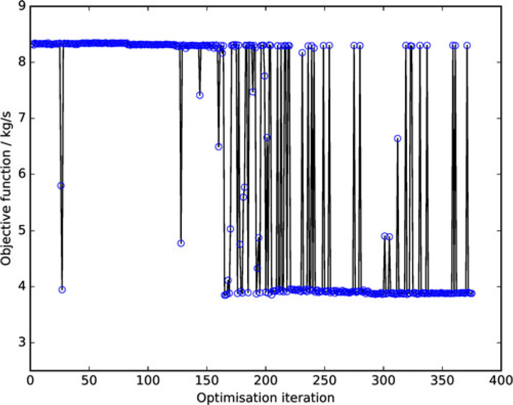
The difficulty with this approach is that a significant portion of the designs are critically separated, and therefore the optimisation can find it difficult to converge. The binary nature of the objective function of designs that are critically separated or not can clearly be seen in Figure 28, which shows the optimisation history for  $\alpha_{\textit{crit}}$+3
 $^\circ$. Despite the apparent difficulty of the process, the optimiser managed to find and guide the search towards non-critically-separated designs, and the same is true for each of the incidences tested. It can be seen in Figure 28 that almost all of the first 100 designs tested are critically separated (i.e. have a high objective function value), but due to the optimiser finding a few feasible designs, it is able to move the search in a beneficial direction. By the end of the optimisation, it can be seen that the majority of the designs are not critically separated. This shows that, despite a steady simulation approach being used to simulate these largely separated designs, the simulation is still able to identify designs that are not critically separated, the objective function recognises this and the optimiser is able to identify and move the search towards designs that reduce separation.
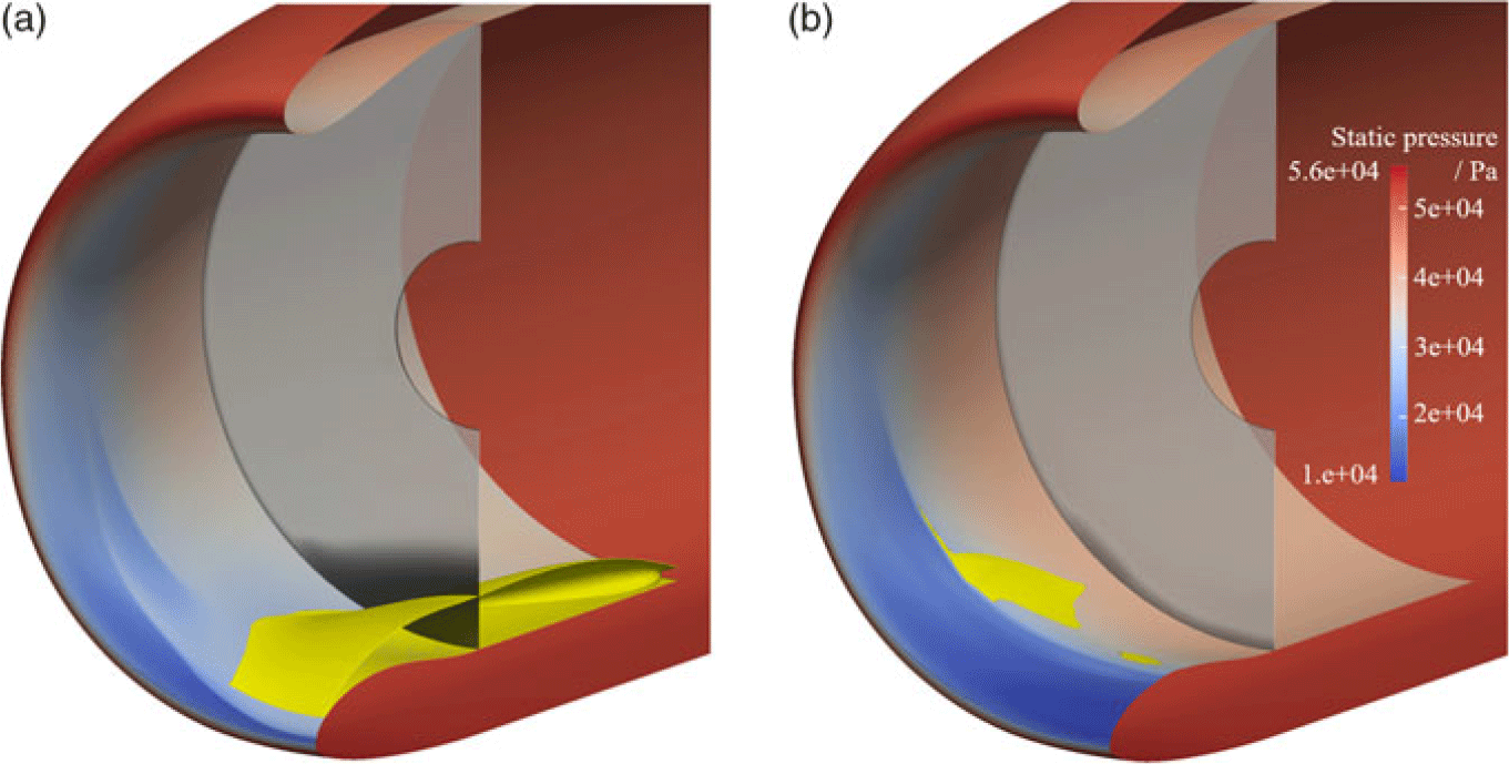
The shock position (static pressure contours), separation (yellow regions) and fan face blockage (dark regions indicate high entropy) for the (a) datum and (b)  $\alpha_{\textit{crit}}$+2
 $^\circ$ optimised geometries at
 $\alpha_{\textit{crit}}$+2
 $^\circ$.

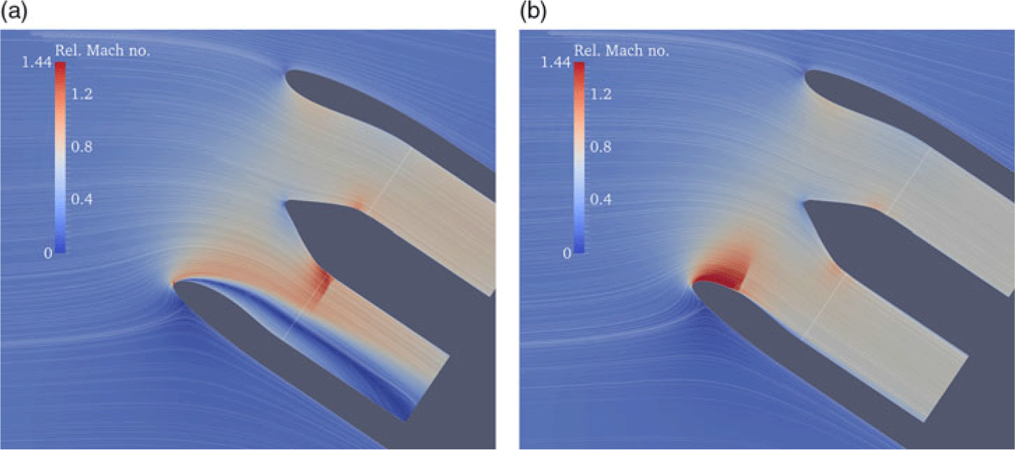
Relative Mach number contour with flow streamlines at  $\theta$ = 0,
 $\alpha_{\textit{crit}}$+2
 $^\circ$ for the (a) datum and (b)
 $\alpha_{\textit{crit}}$+2
 $^\circ$ optimised geometries.

Figures 29 and 30 show the flow features of the  $\alpha_{\textit{crit}}$+2
 $^\circ$ optimised design compared with the datum at
 $\alpha_{\textit{crit}}$+2
 $^\circ$. It can be seen that the optimised design prevents the large separation from occurring, and the blockage at the fan face (shown by the entropy contour in Figure 29) is minimised. Some small region of separation is present, but this is only small compared with the critically separated datum design. The presence of the bump stabilises the shock position, dramatically reducing the separation. Figure 30 shows the datum and optimised geometries rotated to their true orientation at
 $\alpha_{\textit{crit}}$+2
 $^\circ$, with the incoming flow entering horizontally. It can be seen how the addition of the optimised bump stabilises the shock and allows the flow to remain attached at this operating condition. The process is repeated and found to be successful at
 $\alpha_{\textit{crit}}$+3
 $^\circ$ also, providing a
 $3^\circ$ increase in critical incidence. Higher incidence values than this are not tested, but may also be successful.
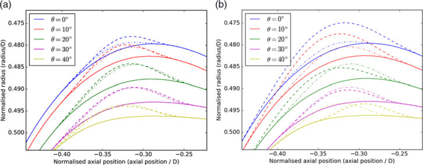
Figure 31 shows the  $\alpha_{\textit{crit}}$+2
 $^\circ$ and
 $\alpha_{\textit{crit}}$+3
 $^\circ$ optimised geometries compared with the datum and the
 $\alpha_{\textit{crit}}$−1
 $^\circ$ optimised geometry. The normalised axial position of the shock for the datum geometry near to separation is around
 $-0.35$ (axial position/D). Figure 31 shows how the bump geometries are all designed with their peak shortly after this point. This was demonstrated previously in the literature to be the best practice for reducing shock strength, and is confirmed again here. It can be seen that there is not much difference between the
 $\alpha_{\textit{crit}}$−1
 $^\circ$ and
 $\alpha_{\textit{crit}}$+2
 $^\circ$ optimised geometries apart from close to bottom dead centre (
 $\theta = 0^\circ$). This indicates how critical this region is for controlling separation.
Constant-theta slices for the datum geometry (solid) and the  $\alpha_{\textit{crit}}$−1
 $^\circ$ optimised geometry (dot dash) plus the (a)
 $\alpha_{\textit{crit}}$+2
 $^\circ$ and (b)
 $\alpha_{\textit{crit}}$+3
 $^\circ$ optimised geometries (dash).

5.2 The achieved increase in critical incidence and further considerations
Figure 32 shows a comparison of the performance of various optimised designs at a range of incidence angles. It can be seen that an increase in critical incidence of at least  $3^\circ$ can be achieved through the use of shock control bumps. It can also be seen how the optimised geometries perform best around the region at which they were designed, but under-perform compared with the datum at lower incidence angles.
Variation in normalised total pressure loss at the fan face with angle-of-attack for the various optimised geometries.

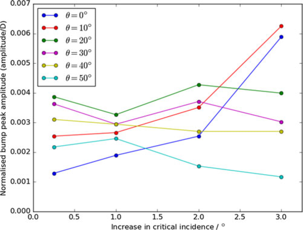
Figure 33 shows a comparison of the bump peak magnitudes at the various circumferential positions for the  $\alpha_{\textit{crit}}$−1
 $^\circ$,
 $\alpha_{\textit{crit}}$+1
 $^\circ$,
 $\alpha_{\textit{crit}}$+2
 $^\circ$ and
 $\alpha_{\textit{crit}}$+3
 $^\circ$ optimised geometries. These are plotted against the achieved increase in critical incidence for each design. It can be seen that, for
 $\theta = 20-50^\circ$, the peak bump amplitude is larger for lower theta values (larger bumps are needed towards bottom dead centre) and there is no strong trend with critical incidence increase. This is not true for
 $\theta = 0^\circ$ and
 $\theta = 10^\circ$ however, where there is a clear trend of increasing bump amplitude with increasing critical incidence benefit. The bumps at these positions go from being the smallest to the largest as the critical incidence benefit increases. This shows that the key difference between the designs’ ability to control separation at high incidence is the bump geometry close to bottom dead centre.
Peak bump amplitude versus achieved increase in critical incidence at various theta positions for the optimised designs.

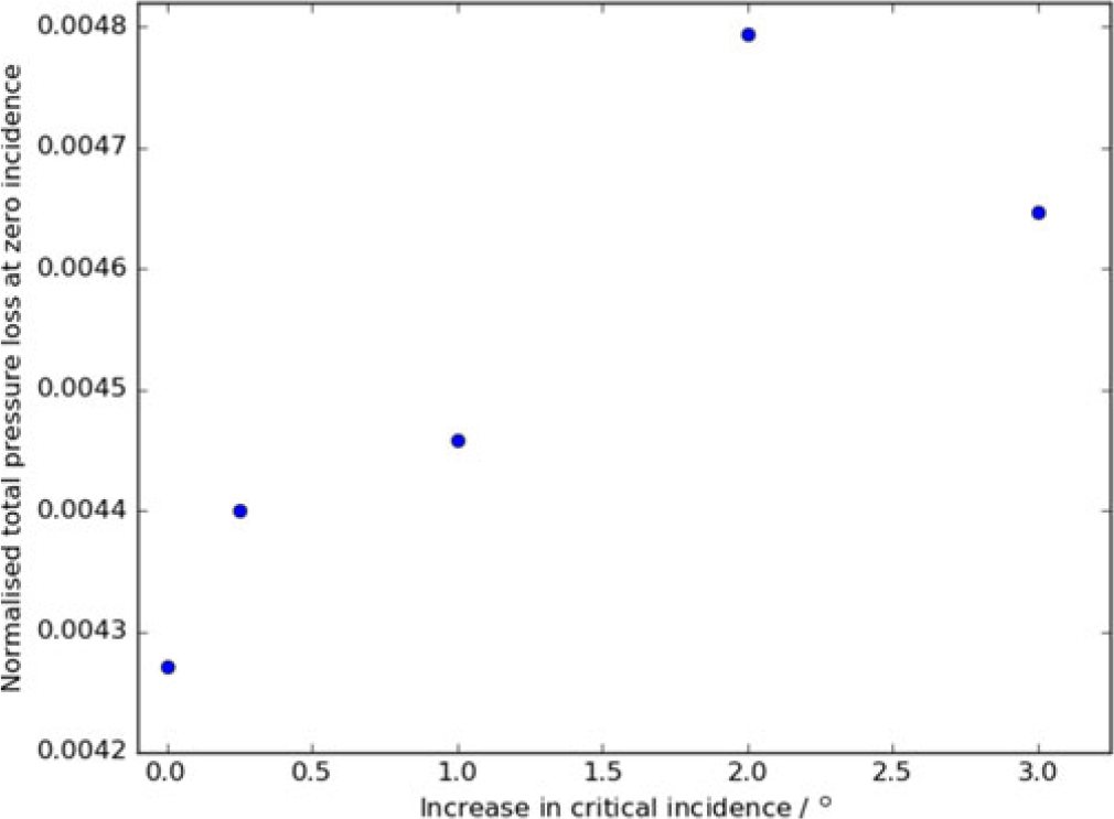
Zero-incidence total pressure loss versus achieved increase in critical incidence for the various optimised geometries.

The higher the angle-of-attack at which the geometry is optimised, the greater its predicted operating range, but the greater its pressure loss at lower incidence angles. This can be seen in Figure 32 for a range of incidence angles, though the zero-incidence condition ( $\alpha = 0^\circ$) is not shown and would not be clearly visible on this scale. Figure 34 gives the normalised total pressure loss through the inlet at
 $\alpha = 0^\circ$ for the various optimised designs, plotted against the achieved increase in critical incidence for that design. This shows how an increase in critical incidence comes at the cost of increased pressure loss at zero incidence, with an achieved increase in critical incidence of 3
 $^\circ$ resulting in approximately a 9% increase in zero-incidence pressure loss.
As mentioned above though, it may be advantageous to trade off a small increase in pressure loss and fuel consumption at lower incidence for the opportunity to use a design that can operate safely at higher incidences using bumps. Alternatively, this could allow the redesign of the intake to be more aggressive (shorter/thinner and therefore lighter and with less drag, which would normally reduce the intake’s critical incidence) with the bumps, ensuring the same operating range is maintained. Making the intake shorter and thinner can provide a significant reduction in nacelle drag(Reference Peters, Spakovszky, Lord and Rose7), which could more than offset the zero-incidence engine performance decrease due to the addition of bumps.
6.0 CONCLUSIONS
This work demonstrates that shock control bumps can be used to alleviate shock-induced separation on engine intakes and that shock control bumps have the ability to increase the safe operating range of the intake. It has been shown that the bump design can be optimised to completely eliminate shock-induced separation at a condition close to the limit of the intake’s operating range. The shock strength can be reduced by around 75% across a range of circumferential positions on the nacelle.
The bump designed at an incidence close to the intake’s limit is able to provide a small increase in critical incidence, but the most success was achieved by optimising bumps at their desired maximum incidence angle. Despite a large number of designs being critically separated, the optimiser combined with steady RANS simulations is able to identify and find designs that reduce separation and allow the flow to remain attached to the intake.
Various conclusions can be drawn from the results presented: The bumps should be allowed as much geometrical freedom as possible to allow them to achieve maximum benefit. The bump peak should be positioned just downstream of the datum shock position, as shown in previous work. The key circumferential region close to the critical incidence is between 30 $^\circ$ and 40
 $^\circ$, due to the localised separation bubble in this region. The key circumferential position for achieving significant increase in critical incidence however is close to bottom dead centre. The greater the desired operational incidence, the greater the bump peak amplitude in this region should be.
Shock control bumps have the potential to increase the incidence beyond which critical separation occurs by at least  $3^\circ$. The optimiser is able to find designs with stable behaviour and reduced separation, providing a significant pressure loss reduction.
Bumps designed at high incidence significantly outperform the datum geometry at this condition, but result in increased pressure loss at lower incidence angles and the cruise condition. The corresponding decrease in engine performance due to the addition of bumps could potentially be offset by the bumps allowing the redesign of the inlet to be shorter/thinner (with less drag) but with the same operating range.
In future work it might be desirable to include the fan in the simulation set-up (which would be expected to influence the separation behaviour), investigate multi-point optimisation/adaptive bumps and redesign an engine intake with reduced drag but using bumps to maintain the same operating range.
ACKNOWLEDGEMENT
The first author is grateful to the Royal Aeronautical Society for the centennial scholarship that supported this research. The authors would also like to thank Rolls-Royce for their support and permission to publish the paper.
SUPPLEMENTARY MATERIAL
To view supplementary material for this article, please visit https://doi.org/10.1017/aer.2020.87