I. INTRODUCTION
High-performance and compact-size low-pass filters (LPFs) with broad stop-band and sharp cut-off frequency are highly in demand in many communication systems, especially in wireless and mobile communications in order to suppress high-frequency harmonics [Reference Hong and Lancaster1]. In [Reference Vamsi and Subrata2], a LPF using shunt open-stubs at feed points of a center fed coupled-line hairpin resonator was presented. This filter had a wide stop-band, but the cut-off frequency was not amply sharp. In [Reference Karimi, Lalbakhsh and Siahkamari3], a LPF with bended resonators and open stubs was presented so as to achieve sharp roll-off and ultra-wide stop-band, even though the structure of the filter was not symmetrical. In [Reference Kaixue and Kiat4], a new transformed radial stubs (TRSs) with an extended stop-band was introduced. In [Reference Wang, Xu, Zhao, Guo and Wu5], a new microstrip LPF with compact size and an ultra-wide stop-band using both triangular patch resonators and radial patch resonators was presented. Sharp roll-off and wide stop-band LPF based on radial split ring was presented in [Reference Hayati, Asadbeigi and Sheikhi6]. A compact LPF using T-shaped patches with an extended stop-band and high suppression factor (SF) was designed in [Reference Sariri, Rahmani, Lalbakhsh and Majidifar7]. In [Reference Wang, Ge, Guo and Wu8], a symmetrical miniaturized LPF using triangular and high-low impedance resonators was introduced. A LPF using a high-impedance bended transmission line loaded by polygonal and triangular resonators was introduced for achieving a good roll-off rate and ultra-wide stop-band [Reference Hayati, Abdipour and Abdipour9].
A novel configuration of shunt stubs and transmission line is presented to improve feature of filter like relative stop-band bandwidth (RSB) size of circuit and figure of merit (FOM) in this paper. Also, the sharpness in transition band is calculated using LC equivalent circuit. The designed filter has an ultra-wide stop-band from 1.79 up to 20.58 GHz with an attenuation level better than −22 dB. The transition band is from 1.47 to 1.77 GHz with −3 and −20 dB, respectively.
II. EQUIVALENT CIRCUIT
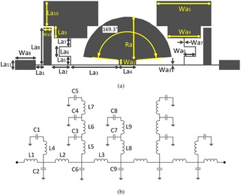
Figure 1(a) shows the topology of the proposed filter, comprises a radial patch resonator, modified T-shaped resonators, and rectangular shaped resonators. The proposed filter combine some resonators, each of which can generate several transmission zeros. The transmission zeros can ameliorate the sharpness in transition band or extend the breadth of stop-band. The modified T-shaped resonators are exploited to achieve sharpness in transition band and the radial patch resonator and rectangular shaped resonators are adopted to attain wide stop-band along with low insertion loss in the transition band. Moreover, the resonators can generate some poles to decrease insertion loss in passband. The LC equivalent circuit of the filter is complex. Thus, the capacitances and inductances effective at high frequencies are omitted in as much as they are not effective for calculating sharpness in transition band as well as transmission zeros at low frequency. The equivalent LC circuit of the filter is illustrated in Fig. 1(b) in which L 2–L 9 are inductances of high–low impedance lossless line and L 1 refers to the inductance of the transmission line. Furthermore, in this figure, capacitors are the sum of equivalent capacitances of microstrip T junction (capacitors are only used) and high–low impedance lossless lines apart from C 1, C 5, and C 8, which are the sum of equivalent capacitances of open-end and high–low impedance lossless line.
(a) Layout of the proposed resonator, (b) the LC equivalent circuit.

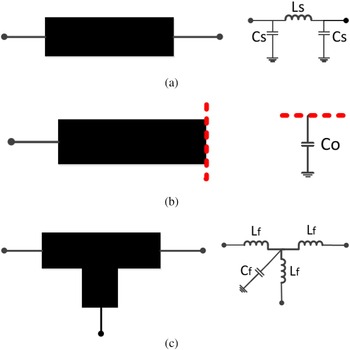
The layout and LC equivalent circuit of high–low impedance lossless line, microstrip line T-junction, and open-end are illustrated in Fig. 2. The Formulas of high–low impedance lossless line are summarized in the figure. Also, the formulas of open-end and microstrip T junction are summarized in [Reference Hong and Lancaster1] and [Reference Wadell10], respectively.
Layout and LC equivalent circuit of: (a) the high–low impedance lossless line, (b) the open-end, (c) the microstrip line T-junction.

A high-impedance lossless line terminated at both ends by relatively low-impedance lines can be presented by a Π-equivalent circuit, as shown in Fig. 2(a). The values of inductors and capacitors can be obtained as:
 $$l_s = \displaystyle{1 \over \omega} \times z_s \times \sin \left( {\displaystyle{{2\pi} \over {\lambda _g}} l} \right),$$
 $$c_s = \displaystyle{1 \over \omega} \times \displaystyle{1 \over {z_s}} \times \tan \left( {\displaystyle{\pi \over {\lambda _g}} l} \right),$$
where z s is the characteristic impedance of the line, l is the length of it, and λ g is the guided wavelength at the cut-off frequency.
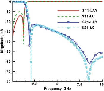
The parameters associated with these structures are L a1 = 0.9 mm, L a2 = 2.25 mm, L a3 = 5.75 mm, L a4 = 2 mm, L a5 = 0.9 mm, L a6 = 1.1 mm, L a7 = 0.95 mm, L a8 = 4.45 mm, L a9 = 1.5 mm, L a10 = 3 mm, L a11 = 1.16 mm, R a = 5.2 mm, W a1 = 1 mm, W a2 = 0.55 mm, W a3 = 0.1 mm, W a4 = 4 mm, W a5 = 6.6 mm, W a6 = 0.1 mm, W a7 = 1.3 mm, and W a8 = 2.5 mm. The values of these parameters can be extracted using Fig. 2. They are tabulated in Table 1. Figure 3 shows frequency response of the proposed filter and EM and equivalent circuit simulation results of proposed filter which are in good agreement.
EM and equivalent circuit simulation results of the proposed filter.

Calculated values for LC equivalent circuit (Units: C, pF; L, nH).

In this section, we will look at the behavior of the main resonator by examining its transfer function. The transfer function is calculated from LC equivalent circuit, for example, sharpness in the transition band can be adjusted with transfer function. r in the transfer function alludes to resistance of matching. Also note that s = jω.
 $$\displaystyle{{v_o} \over {v_i}} _{T\_sh} = \displaystyle{{\left( {a^2 b^2 cr} \right)} \over {\left( \matrix{\left( {s\left( {r + L_1 s} \right)\left( {b\left( {L_2 + L_3} \right) + L_2 L_3 s} \right) + a\left( {L_3 s\left( {r + \left( {L_1 + L_2} \right)s} \right) + b\left( {r + \left( {L_1 + L_2 + L_3} \right)s} \right)} \right)} \right) \hfill \cr \times \left( {\left( {r + L_1 s} \right)\left( {2bc + b\left( {L_2 + L_3} \right)s + L_2 s\left( {2s + L_3 s} \right)} \right) + a\left( {\left( {r + \left( {L_1 + L_2} \right)s} \right)\left( {2c + L_3 s} \right) + b\left( {2c + r + \left( {L_1 + L_2 + L_3} \right)s} \right)} \right)} \right) \hfill} \right)}}, $$
where
 $$a = \displaystyle{{1 + C_1 L_4 s^2} \over {C_1 s + C_2 s + C_1 C_2 L_4 s^3}}, $$
 $$b = \displaystyle{{\left( {1 + s^2 \left( {C_5 \left( {L_5 + L_6 + L_7} \right) + C_4 \left( {L_5 + L_6} \right)\left( {1 + C_5 L_7 s^2} \right) + C_3 L_5 \left( {1 + \left( {C_4 L_6 + C_5 \left( {L_6 + L_7} \right)} \right)s^2 + C_4 C_5 L_6 L_7 s^4} \right)} \right)} \right)} \over {\left( {s\left( \matrix{C_5 + C_6 + C_5 C_6 \left( {L_5 + L_6 + L_7} \right)s^2 + C_4 \left( {1 + C_6 \left( {L_5 + L_6} \right)s^2} \right) \hfill \cr \left( {1 + C_5 L_7 s^2} \right) + C_3 \left( {1 + C_6 L_5 s^2} \right)\left( {1 + \left( {C_4 L_6 + C_5 \left( {L_6 + L_7} \right)} \right)s^2 + C_4 C_5 L_6 L_7 s^4} \right) \hfill} \right)} \right)}},$$
 $$c = \displaystyle{{1 + (C_7 L_8 + C_8 (L_8 + L_9 ))s^2 + C_7 C_8 L_8 L_9 s^4} \over {s(C_8 + C_9 + C_8 C_9 (L_8 + L_9 ))s^2 + C_7 (1 + C_9 C_8 s^2 )(1 + C_8 L_9 s^2 )}}.$$
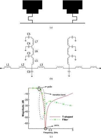
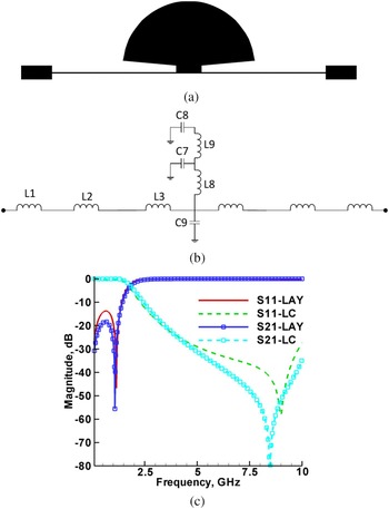
Figure 4(a) shows the structure of modified T-shaped resonators. The equivalent LC circuit of the modified T-shaped resonators is shown in Fig. 4(b). In Fig. 4(c), frequency responses of the proposed filter and modified T-shaped resonators are compared with one another. It can be seen that the steep sharpness in transition band is generated by modified T-shaped resonators. Hence, in this paper, we utilized LC model and transfer function of modified T-shaped resonators for the calculation and enhancement of the sharpness in transition band because the transfer function can be calculated by the LC model. Furthermore, we have calculated the frequency of pole and zero (they are seen in Fig. 4(c)) through the transfer function. The sharpness is equated to zero frequency minus pole frequency. The formula of sharpness is summarized here. The formula of sharpness is used to achieve the best sharpness in transition band. For instance, the sharpness can be changed and improved by altering L 3. L 3 changes by altering L a3 and W a3. As a result, the sharpness is simply adjustable. For example, if L 3 was 4.8, 4.3, and 3.8 nH, L a3 will be 6.25, 6, and 5.75, respectively. Therefore, sharpness (f 20 db − f 3 db) will be 0.48, 0.45, and 0.4 GHz and choosing suitable dimension for designing a suitable sharpness is simple.
(a) Layout of the T-shaped resonators, (b) LC equivalent circuit of the T-shaped resonators, (c) frequency responses of the proposed filter and T-shaped resonators.

 $$sharpness\approx \left\vert \matrix{\displaystyle{{ - \displaystyle{r \over {3L_1}} +\left( {1 + \sqrt { - 3}} \right)\left( {3dL_1 L_2 \left( {2L_1 + L_2} \right) - d^2 L_2^2 r^2} \right)} \over {\left( \matrix{3\left( {2^{2/3} dL_1L_2} \right)\left( \matrix{ - 36d^2 L_1^2 L_2^2 r + 9d^2 L_2 L_2^3 r -2d^{^{_3}} L_2^3 r^3 \hfill \cr + \sqrt {4\left( {3dL_1 L_2 \left( {2L_1 +L_2} \right) - d^2 L_2^2 r^2} \right)^3 + \left( { - 36d^2 L_1^2 L_2^2 r +9d^2 L_1 L_2^3 r - 2d^3 L_2^3 r^3} \right)^2} \hfill} \right)^{1/3} \hfill\cr - \displaystyle{1 \over {6\left( {2^{1/3} dL_1 L_2} \right)}}\left( {1 -\sqrt { - 3}} \right)\left( \matrix{ - 36d^2 L_1^2 L_2^2 r + 9d^2 L_1 L_2^3 r- 2d^3 L_2^3 r^3 \hfill \cr + \sqrt {\left( {4\left( {3dL_1 L_2 \left( {2L_1+ L{}_2} \right) - d^2 L_2^2 r^2} \right)^3 + \left( { - 36d^2 L_1^2 L_2^2 r+ 9d^2 L_1 L_2^3 r - 2d^3 L_2^3 r^3} \right)^2} \right)} \hfill}\right)^{1/3} \hfill} \right)}} \hfill \cr - \displaystyle{1 \over {\sqrt{L_5 (C_3 + C_4 + C_5 ) + L_6 (C_4 + C_5 ) + C_5 L_7}}} \hfill} \right\vert, $$
where
 $$d = C_4 + C_5 + 3C_6 + \displaystyle{7 \over 6}C_3. $$
Figure 4(c) shows frequency response of modified T-shaped resonators, but the structure does not have a suitable stop-band. To increase stop-band, a strong transmission zero is generated by the radial patch resonator and it is incorporated into the modified T-shaped resonators. Figure 5(a) shows the structure of radial resonator and its equivalent LC circuit and frequency response are shown in Figs 5(b) and 5(c).
(a) Layout of the radial patch resonator, (b) LC equivalent circuit of the radial patch resonator, (c) frequency responses of layout and LC equivalent circuit of the radial patch resonator.

The transfer function of radial patch resonator is computed to achieve the transmission zero of radial patch resonator.
 $$\displaystyle{{v_o} \over {v_i}} _{rad.} = \displaystyle{{ - (r(1 + C_7 L_8 s^2 + C_8 L_8 + C_8 L_9 s^2 + C_7 C_8 L_8 L_9 s^4 ))} \over \matrix{((r(1 + L_a s)(C_7 s + C_8 s + C_7 C_9 L_8 s^3 + C_8 C_9 L_8 s^3 + C_7 C_8 L_9 s^3 + C_7 C_8 C_9 L_8 L_9 s^5 ). \times \hfill \cr (r + L_a s + \displaystyle{{2(1 + C_7 L_8 s^2 + C_8 L_8 S^2 + C_8 L_9 s^2 + C_7 C_8 L_8 L_9 s^4 )} \over {C_7 s + C_8 s + C_9 s + C_7 C_9 L_8 s^3 + C_8 C_9 L_8 s^3 + C_7 C_8 L_9 s^3 + C_8 C_9 L_9 s^3 + C_7 C_8 C_9 L_8 L_9 s^5}} )) \hfill}}, $$
where
 $$L_a = L_1 + L_2 + L_3. $$
The transmission zero can be calculated by equation (5)
 $$F_z = \left\vert {\displaystyle{{\sqrt { - (1/C_7 L_8 ) - (1/C_7 L_9 ) - (1/C_8 L_9 ) - \left(\sqrt { - 4C_7 C_8 L_8 L_9 + \left( {C_7 L_8 + C_8 L_8 + C_8 L_9} \right)^2} /C_7 C_8 L_8 L_9 \right)}} \over {2\sqrt {2\pi}}}} \right\vert.$$
The location of transmission zeros can easily be changed. For example, the location of transmission zeros is related to L 7 in Fig. 5(b) and L 7 changes by altering W a2 in Fig. 1(a). Also, W a2 has the direct relevance with the location of transmission zero.
III. SIMULATION AND EXPRIMENTAL RESULTS
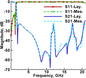
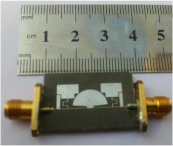
Figure 6 shows the results of simulation and measurement. Simulated and measured results are obtained by an EM-simulator advanced design system (ADS) and Agilent network analyzer N5230A, respectively. Evidently, return loss and insertion loss are better than 13.1 and 0.4 dB from DC to 1.3 GHz, respectively. The results exhibit that the stop-band with 22 dB as a reference is from 1.8 up to 20.6 GHz and the sharpness in transition band is roughly 0.269 GHz (1.474–1.906 GHz with −3 and −40 dB, respectively). Figure 7 shows the photograph of the presented filter fabricated on a substrate with a relative dielectric constant ε r = 2.2, thickness h = 15 mil, and loss tangent tand = 0.0009 (RT/duroid 5880). The size of the fabricated LPF is about 22 × 7.75 mm2, which corresponds to an electrical size of 0.147 × 0.052 λ g , where λ g is the guided wavelength at 1.47 GHz.
Simulated and measured performance of the LPF.

Photograph of the proposed filter.

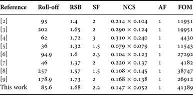
For comparison, Table 2 provides a summary of some LPF performances based on several specifications defined in [Reference Hayati, Asadbeigi and Sheikhi6]. As shown in the Table 2, the presented filter demonstrates much higher FOM (41389) than the quoted filters. The following paragraphs define some relevant parameters.
Performance comparison among published filters and presented one.
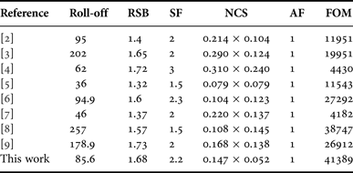
Sharp roll-off (ξ) is a parameter for defining sharpness in transition band.
 $$\xi = \displaystyle{{\alpha _{max} - \alpha _{min}} \over {f_s - f_c}} ({\rm dB/GHz}),$$
where α max is the 40 dB attenuation point, α min is the 3 dB attenuation point, f s is the 40 dB stop-band frequency, and f c is the 3 dB cut-off frequency. TheRSB is given by:
 $${\rm RSB =} \displaystyle{{{\rm stop - band}\,\,{\rm bandwidth}} \over {{\rm stop - band}\,\,{\rm center}\,\,{\rm frequency}}}. $$
The SF is based on the stop-band bandwidth. For example, the stop-band bandwidth is referred to 22 dB suppression, thus the corresponding SF is defined as 2.2. A higher suppression corresponds to a greater SF. The normalized circuit size (NCS) is calculated by:
 $${\rm NCS =} \displaystyle{{{\rm physical}\,\,{\rm size}\,{\rm (length} \times {\rm width)}} \over {\lambda _g^2}},$$
where λ g is the guided wavelength at 3 dB cut-off frequency. The architecture factor (AF) can be recognized as the circuit complexity factor, which is:
 $${\rm FOM} = \displaystyle{{\varepsilon \times {\rm RSB} \times {\rm SF}} \over {{\rm NCS} \times {\rm AF}}}.$$
IV. CONCLUSION
A novel microstrip LPF with small size and ultra-wide stop-band is presented. In this paper, sharpness, transmission zero, and transfer function have been calculated and examined. The presented filter has a very high FOM of 41389. Considering all these good properties, the proposed LPF is applicable in modern communication systems.
 Hesam Siahkamari was born in Kermanshah, Iran in 1988. He received his B.Sc. degree in Electronic Engineering in 2010 from Islamic Azad University, Kermanshah, Iran and M.Sc. degree in Electronic Engineering in 2013 from Razi University, Kermanshah, Iran. His current research interest includes RF/Microwave circuit design.
 Ehsan Heidarinezhad was born in Kermanshah, Iran, in 1986. He received his B.S. degree in Electronics Engineering from Islamic Azad University, Kermanshah Branch, Kermanshah, Iran, in 2009, and his M.S. degree in Electrical Engineering from the Islamic Azad University, Science and Research, Kermanshah Branch, Kermanshah, Iran, in 2014. His current research interest includes RF/Microwave circuit design.
 Ehsan Zarayeneh was born in Kermanshah, Iran in 1987. He received his B.S. degree in Electronics Engineering in 2011 from Islamic Azad University, Toyserkan Branch, Hamedan, Iran and he received his M.S. degree in Electronics Engineering from Islamic Azad University, South Tehran Branch in 2014, Tehran, Iran. His current research interest includes RF/Microwave circuit design.
 Seyyed Ali Malakooti was born in Tehran Province, Tehran, Iran, in 1987. He received his B.S. and M.S. degrees in Electrical Engineering from Razi University, Kermanshah, Iran, in 2010 and 2013, respectively. In 2015, he joined Unishare Robotic Co., Kermanshah, Iran. His current research interests include design of microstrip antennas, multi-band passive microwave components, and digital-integrated circuits.
 Seyyed Mohammad Hadi Mousavi was born in Kermanshah, Iran, in 1990. He received his B.S. degree in 2012 from Islamic Azad University and the M.S. degree from Islamic Azad University, Science and Research Branch, Kermanshah, Iran, in 2014, all in Communication Engineering. His research interests include high-frequency circuits and Microstrip circuit design.
 Payam Siahkamari was born in Kermanshah, Iran in 1991. He received his B.Sc. degree in Electronic Engineering in 2015 from Islamic Azad University, Kermanshah, Iran and he is now pursuing his M.Sc. degree from Islamic Azad University, Science and Research Branch, Kermanshah, Iran. His current research interest includes RF/Microwave circuit design.