1 Introduction
Prediction of laminar–turbulent flow transition and the associated heat transfer in high-speed flows, as well as control of both phenomena, is key to optimizing the performance of next-generation aerospace vehicles. While the instability mechanisms leading to transition on essentially two-dimensional flows, such as the flat-plate boundary layer or flow around a circular cone at zero angle of attack, are well studied both experimentally and theoretically (Mack Reference Mack1984; Stetson & Kimmel Reference Stetson and Kimmel1992; Schneider Reference Schneider2004; Fedorov Reference Fedorov2011; Schneider Reference Schneider2015), instability analyses of three-dimensional boundary layers in hypersonic flow have only commenced recently. The distinction must be made here regarding boundary-layer flows in which the velocity vector comprises all three components, which are functions of the single inhomogeneous spatial direction, namely along the wall-normal (e.g. infinite swept wing boundary-layer flow), and flows in which two essentially inhomogeneous spatial directions exist. Confusingly, both classes of such flows are referred to in the literature as three-dimensional boundary layers. However, while classic local linear stability theory (LST) (Mack Reference Mack1984) and parabolized stability equations (PSE) (Herbert Reference Herbert1997) are appropriate tools to study the flow instability in the former class of flows, multi-dimensional global linear theory (Theofilis Reference Theofilis2011) must be used in the context of the latter class of flows.
Study of instability mechanisms in three-dimensional boundary layers is essential in order to advance current understanding of the transition process on realistic vehicles, since a number of differences exist between three-dimensional and two-dimensional and axisymmetric geometries. Instabilities other than the plane waves typically amplified in two-dimensional and axisymmetric flows may become unstable and lead three-dimensional boundary-layer flow to transition; cross-flow instabilities are a prime example of this class (Reed & Saric Reference Reed and Saric1989; Reed, Saric & Arnal Reference Reed, Saric and Arnal1996; Saric, Reed & White Reference Saric, Reed and White2003; Li & Choudhari Reference Li and Choudhari2011). In addition, high-frequency second-mode instabilities are also present in three-dimensional boundary layers. Balakumar & Reed (Reference Balakumar and Reed1991) identified oblique second Mack modes in the three-dimensional supersonic boundary layer formed over a rotating cone at zero angle of attack and Mach numbers
 $5$
and
 $8$
.
Near-wall streamlines along an aspect ratio
 $2\,:\,1$
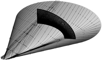
elliptic cone, showing motion of the fluid from the attachment line towards the centreline. The roll-up of streamlines over the centreline leads to a strongly and azimuthally non-parallel flow near the minor axis. Also shown is one of the planes on which spatial BiGlobal instability analysis has been performed.

The mentioned classes of three-dimensional boundary-layer flow instabilities co-exist in the elliptic cone. Figure 1 shows near-wall streamlines on the elliptic cone at the conditions presently studied. The three-dimensionality of the geometry inevitably produces spanwise (azimuthal in the present geometry) pressure gradients which, in turn, induce cross-flow, that is fluid from the leading edge being moved towards the centreline. Streamlines diverge from the attachment line towards the minor-axis centreline, where a pair of counter-rotating vortices is formed. In the area of the cone between the attachment line and the centreline, the low-momentum fluid near the surface is deflected more than the fluid near the edge of the boundary layer, resulting in a inflectional velocity profile. Under these conditions, cross-flow vortices may be established inside the three-dimensional boundary layer, and on occasion dominate the transition process.
The hypersonic international flight research experimentation (HIFiRE) programme (Kimmel et al.
Reference Kimmel, Adamczak, Berger and Choudhari2010) has employed two conical geometries in both flight testing and ground experiments. The HIFiRE-5 test vehicle is a
 $2\,:\,1$
elliptic cone model with a rounded nose tip. The main property of this geometry is that a three-dimensional boundary layer develops at zero angles of attack and yaw. The present analysis focuses on this configuration.
Efforts to understand laminar–turbulent transition on elliptic cones have mostly employed cones of aspect ratios
 $2\,:\,1$
and
 $4\,:\,1$
, exposed at zero angle of attack to oncoming flows for Mach numbers (
 $M$
) between
 $4$
and
 $8$
. Early experimentation of Schmisseur, Schneider & Collicott (Reference Schmisseur, Schneider and Collicott1998, Reference Schmisseur, Schneider and Collicott1999) reported that the minor-axis centreline area was the most receptive to amplification of perturbations in a
 $4\,:\,1$
elliptic cone at
 $M=4$
. The experiments of Poggie & Kimmel (Reference Poggie and Kimmel1998) produced evidence of the classical cross-flow and second Mack mode instabilities in a
 $2\,:\,1$
elliptic cone at
 $M=8$
; they observed early transition near the semi-minor-axis centreline and delayed transition near the leading edge. Huntley & Smits (Reference Huntley and Smits2000) and Huntley (Reference Huntley2000) employed filtered Rayleigh scattering and produced images of the early stages of transition on sharp-nosed
 $4\,:\,1$
and
 $2\,:\,1$
elliptic cones also at
 $M=8$
, demonstrating that transition begins with the emergence of small-scale structures near the minor-axis centreline of the cone, rather than in the outboard cross-flow or leading-edge regions.
More recently, great insight has been provided by the ground experiments carried out in the Boeing/AFOSR Mach-6 Quiet Tunnel at Purdue University (Schneider Reference Schneider2008). Juliano & Schneider (Reference Juliano and Schneider2010) presented the first wind-tunnel results of the HIFiRE-5 geometry on this experimental facility. They measured heat flux and boundary-layer transition by means of temperature-sensitive paint. Transition was observed along the centreline and roughly half-way between the centreline and leading edge. The transition on the centreline was suspected to arise from the amplification of second-mode waves in the inflected centreline boundary-layer profile, while the second case was suspected to be due to the breakdown of cross-flow vortices. These observations were restated in a later work by Juliano, Borg & Schneider (Reference Juliano, Borg and Schneider2015b ), in which they included the increase of the angle of attack from 0 to 4 deg, observing how the transition front induced by cross-flow instability moved downstream on the windward side for increasing angle of attack. Further experiments in the same quiet tunnel were conducted by Borg, Kimmel & Stanfield (Reference Borg, Kimmel and Stanfield2011), who reported stationary and travelling cross-flow waves under quiet flow conditions. Roughness-induced transition was also investigated on the attachment line, concluding that three-dimensional roughness elements destabilize more than two-dimensional roughness elements. Borg, Kimmel & Stanfield (Reference Borg, Kimmel and Stanfield2012) focused on the study of cross-flow disturbances. While stationary and travelling waves were simultaneously observed under quiet flow conditions, no travelling disturbances were detected with noisy flow.
Later on, Borg, Kimmel & Stanfield (Reference Borg, Kimmel and Stanfield2015) continued the study of travelling cross-flow disturbances in the same Mach-6 quiet tunnel. The phase speed and wave angle were calculated from the cross-spectra of three pressure sensors located in the area of the cone between the leading edge and the centreline. Both quantities showed good agreement with classic LST. An interesting finding was that when running the experimental facility in noisy flow conditions, transition along the surface of the cone occurred for a much lower Reynolds number than in quiet flow. The authors reported that breakdown of travelling cross-flow instabilities was not the primary transition mechanism under noisy conditions. The instability mechanism that causes laminar–turbulent transition at noisy flow conditions is still unclear.
A remarkable effort is the HIFiRE-5 flight test in April 2012. Although the upper stage of the sounding rocket failed to ignite, achieving a peak Mach number of approximately 3 instead of the target of 7, previous experimental and numerical predictions were confirmed. The analysis of the collected flight data was first reported by Kimmel, Adamczak & Juliano (Reference Kimmel, Adamczak and Juliano2013). They showed a transition pattern consistent with prior wind-tunnel measurements and numerical studies. The results confirmed early transition along the minor-axis meridian, while the leading edge experienced transition at higher Reynolds numbers. Juliano, Adamczak & Kimmel (Reference Juliano, Adamczak and Kimmel2014) presented the analysis of the heat flux, which was calculated from paired thermocouples, identifying boundary-layer transition locations from the heating rates. Recently, Juliano, Adamczak & Kimmel (Reference Juliano, Adamczak and Kimmel2015a
) reported a thorough analysis of the flight data, concluding that two boundary-layer transition mechanisms were encountered during the supersonic descent. One mode caused transition over the minor-axis surface of the vehicle and correlated well with body length Reynolds number
 $Re_{x}$
, while the other mechanism caused the leading-edge transition to advance rapidly over a small range of free stream
 $Re^{\prime }$
. These findings increased confidence in the success of a second flight test that is expected to validate the theoretical predictions at flight conditions.
Parallel, large-scale computations performed by Bartkowicz, Subbareddy & Candler (Reference Bartkowicz, Subbareddy and Candler2010) and Dinzl & Candler (Reference Dinzl and Candler2015) have indicated the high level of grid refinement and associated computational requirements needed to study transition phenomena in hypersonic three-dimensional boundary layers, and specifically on the HIFiRE-5 geometry, using direct numerical simulations (DNS). Efficient linear and nonlinear flow instability analyses are required to identify critical conditions for flow instability and to study modal and non-modal scenarios that might produce transition.
In an early effort to analyse flow instability mechanisms on the elliptic cone, Theofilis (Reference Theofilis2002) developed the first global inviscid instability analysis of a compressible flow by solving the appropriate two-dimensional Rayleigh equation. Members of the different branches of the spectrum obtained were identified as modes of hydrodynamic or of aeroacoustic origin in subsonic and supersonic flow, respectively. More recently, Choudhari et al. (Reference Choudhari, Chang, Jentink, Li, Berger, Candler and Kimmel2009) performed a thorough stability analysis of the viscous hypersonic flow over the HIFiRE-5 geometry at ground and flight test conditions using local LST, PSE and spatial BiGlobal analysis. The local LST and PSE stability results, which base the transition prediction on
 $N$
-factor integration along streamlines and grid lines of the elliptic cone, are briefly discussed next. Under flight conditions at an altitude of 18 km,
 $M=7$
, and
 $Re^{\prime }=1.85\times 10^{7}~\text{m}^{-1}$
, the
 $N$
-factor reached values above
 $N=40$
at the end of the cone and along the centreline, attachment line and cross-flow paths. At the higher altitude of 33 km, at which the
 $Re^{\prime }$
is 11 times smaller, the overall
 $N$
-factors were considerably lower, not exceeding the typical transition threshold of approximately
 $N=15$
required in quiet environment conditions (Li et al.
Reference Li, Choudhari, Chang, Kimmel, Adamczak and Smith2015).
Choudhari et al. (Reference Choudhari, Chang, Jentink, Li, Berger, Candler and Kimmel2009) also studied the HIFiRE-5 model at wind-tunnel conditions, i.e.
 $M=6$
and
 $Re^{\prime }=10^{7}~\text{m}^{-1}$
. The model used is
 $38.1\,\%$
scale of the flight test article. In this case,
 $N$
-factors along centreline, attachment line, and cross-flow paths were found to be marginally above
 $10$
at the end for the geometry. This work was continued by Li et al. (Reference Li, Choudhari, Chang, White, Kimmel, Adamczak, Borg, Stanfield and Smith2012), who focused on ground testing conditions. A grid convergence of the mean flow was conducted and
 $N$
-factors based on travelling cross-flow instabilities were computed through local LST and PSE. Good agreement was observed by comparing with the experimental results of Borg et al. (Reference Borg, Kimmel and Stanfield2011). In the same context, Gosse, Kimmel & Johnson (Reference Gosse, Kimmel and Johnson2010), Gosse, Kimmel & Johnson (Reference Gosse, Kimmel and Johnson2014) performed PSE instability analysis of the HIFiRE-5 configuration at four altitudes, i.e.
 $21.8$
,
 $25.0$
,
 $28.3$
and 33.0 km, to provide insights for the flight tests. These authors focused on the major- and minor-axis meridians, finding the same trend of increasing
 $N$
-factors as the altitude decreased and the free-stream unit Reynolds number,
 $Re^{\prime }$
, increased.
 $N$
-factor values were found to be high enough to cause transition along both the centreline and the attachment-line symmetry planes only for the lowest altitude of 21.8 km. In the present work, the mean flow analysed from a global LST point of view is the flow computed by Gosse et al. (Reference Gosse, Kimmel and Johnson2010, Reference Gosse, Kimmel and Johnson2014) at the most relevant altitude case, 21.8 km, in which all the possible instability mechanisms are expected to play a role in the laminar–turbulent transition process.
Focusing now on BiGlobal instability analysis results, Choudhari et al. (Reference Choudhari, Chang, Jentink, Li, Berger, Candler and Kimmel2009) were the first to recover centreline instabilities on the elliptic cone, specifically on the HIFiRE-5 geometry at flight flow conditions for an altitude of 18 km and
 $Re^{\prime }=1.85\times 10^{7}~\text{m}^{-1}$
, by solving a BiGlobal stability eigenvalue problem without curvature effects of the flow in the vicinity of the centreline. They presented the shape functions of four centreline instabilities at a unique axial station,
 $x^{\ast }=0.7~\text{m}$
, and remarked that these modes are a consequence of the three-dimensional high-shear layer surrounding the low-velocity streak formed on the centreline. For the same flight flow conditions, they reported unstable attachment-line instabilities and observed that their amplified frequencies corresponded to second Mack mode frequencies. More recently, Paredes & Theofilis (Reference Paredes and Theofilis2015) performed a spatial BiGlobal study of the HIFiRE-5 model including the curvature effects of the elliptic cone geometry. The flight flow conditions used correspond to an altitude of 33 km and
 $Re^{\prime }=1.89\times 10^{6}~\text{m}^{-1}$
. At this lower
 $Re^{\prime }$
, and in line with the predictions of Choudhari et al. (Reference Choudhari, Chang, Jentink, Li, Berger, Candler and Kimmel2009), attachment-line instabilities were not observed. Indeed, they were not expected to be amplified because the attachment-line Reynolds number correlation (Malik, Li & Choudhari Reference Malik, Li and Choudhari2007) did not exceed the threshold. The study by Paredes & Theofilis (Reference Paredes and Theofilis2015) focused on the centreline instabilities, which at these flow conditions peaked adjacent to the mushroom-like centreline structure at the same locations of maximum base flow shear. Furthermore, oblique second modes were reported in the boundary layer located in the vicinity of the minor-axis meridian in the range of frequencies of the centreline instabilities.
In the present work the spatial BiGlobal analysis technique is used to study the modal instabilities amplified in the hypersonic flow over the HIFiRE-5 elliptic cone geometry. The flow parameters are selected to simulate high-Reynolds-number flight conditions at an altitude of 21.8 km,
 $M=7.45$
, and
 $Re^{\prime }=1.015\times 10^{7}~\text{m}^{-1}$
. BiGlobal analysis theory assumes that the base flow is quasi-parallel, i.e. the base flow components are assumed to be independent of the streamwise coordinate. The present analysis has been performed using an in-house-developed multi-dimensional stability code. This code has been verified against DNS, analysing instability of the wake behind an isolated roughness element in supersonic flow (De Tullio et al.
Reference De Tullio, Paredes, Sandham and Theofilis2013). In the latter work, the first demonstrated plane-marching or three-dimensional parabolized stability equations (PSE-3D) analysis technique (Paredes Reference Paredes2014; Paredes et al.
Reference Paredes, Hanifi, Theofilis and Henningson2015) for high-speed flows was performed, showing excellent agreement of spatial BiGlobal and PSE-3D results when compared with DNS results in the linear regime. Furthermore, Paredes et al. (Reference Paredes, Perez, Reed and Theofilis2014) used the spatial BiGlobal stability analysis code to identify high-frequency or second-mode instabilities responsible for transition on the windward face of a
 $7^{\circ }$
half-angle circular cone at a
 $6^{\circ }$
angle of attack,
 $M=6$
, and
 $Re^{\prime }=1.009\times 10^{7}~\text{m}^{-1}$
. The results agreed well with previous classic LST and PSE calculations by Perez, Reed & Kuehl (Reference Perez, Reed and Kuehl2012) and the experimental measurements of Kroonenberg et al. (Reference Kroonenberg, Radespiel, Candler and Estorf2010).
The spatial BiGlobal equations are introduced for compressible flows and applied to the elliptic cone geometry in § 2. Details of the analysed base flow are discussed in § 3. In the same section, spatial BiGlobal instability analysis results are shown for a wide range of frequencies at different distances from the cone tip. The study mainly focuses on the areas close to the minor-axis and major-axis meridians of the body. Furthermore, multi-dimensional instability analysis tools have been employed for the first time to obtain results on the cross-flow and oblique second Mack mode disturbances, both of which are amplified along the entire surface of the geometry. A summary and concluding remarks are offered in § 4.
2 Instability analysis theory
The analysis of flow stability is based on the compressible equations of motion, written in dimensionless form as
 $$\begin{eqnarray}\displaystyle & \displaystyle \frac{\unicode[STIX]{x2202}\unicode[STIX]{x1D70C}}{\unicode[STIX]{x2202}t}+\unicode[STIX]{x1D735}\boldsymbol{\cdot }(\unicode[STIX]{x1D70C}\boldsymbol{V})=0, & \displaystyle\end{eqnarray}$$
 $$\begin{eqnarray}\displaystyle & \displaystyle \unicode[STIX]{x1D70C}\left[\frac{\unicode[STIX]{x2202}\boldsymbol{V}}{\unicode[STIX]{x2202}t}+(\boldsymbol{V}\boldsymbol{\cdot }\unicode[STIX]{x1D735})\boldsymbol{V}\right]=-\unicode[STIX]{x1D735}p+\frac{1}{Re}\left\{\unicode[STIX]{x1D735}[\unicode[STIX]{x1D706}(\unicode[STIX]{x1D735}\boldsymbol{\cdot }\boldsymbol{V})]+\unicode[STIX]{x1D735}\boldsymbol{\cdot }[\unicode[STIX]{x1D707}((\unicode[STIX]{x1D735}\boldsymbol{V})+(\unicode[STIX]{x1D735}\boldsymbol{V})^{\text{T}})]\right\},\quad & \displaystyle\end{eqnarray}$$
 $$\begin{eqnarray}\displaystyle \unicode[STIX]{x1D70C}\left[\frac{\unicode[STIX]{x2202}T}{\unicode[STIX]{x2202}t}+(\boldsymbol{V}\boldsymbol{\cdot }\unicode[STIX]{x1D735})T\right] & = & \displaystyle \frac{1}{Re\,Pr}\unicode[STIX]{x1D735}\boldsymbol{\cdot }(\unicode[STIX]{x1D705}\unicode[STIX]{x1D735}T)+(\unicode[STIX]{x1D6FE}-1)M^{2}\left[\frac{\unicode[STIX]{x2202}p}{\unicode[STIX]{x2202}t}+(\boldsymbol{V}\boldsymbol{\cdot }\unicode[STIX]{x1D735})p\right]\nonumber\\ \displaystyle & & \displaystyle +\,\frac{(\unicode[STIX]{x1D6FE}-1)M^{2}}{Re}\left\{\unicode[STIX]{x1D706}(\unicode[STIX]{x1D735}\boldsymbol{\cdot }\boldsymbol{V})^{2}+\frac{\unicode[STIX]{x1D707}}{2}[(\unicode[STIX]{x1D735}\boldsymbol{V})+(\unicode[STIX]{x1D735}\boldsymbol{V})^{\text{T}}]^{2}\right\}\end{eqnarray}$$
where
 $\boldsymbol{V}$
is the velocity vector,
 $\unicode[STIX]{x1D70C}$
the density,
 $p$
the pressure,
 $T$
the temperature,
 $M$
the Mach number,
 $Re$
the Reynolds number,
 $Pr$
the Prandtl number,
 $\unicode[STIX]{x1D6FE}$
the specific heat coefficient,
 $\unicode[STIX]{x1D705}$
the thermal conductivity,
 $\unicode[STIX]{x1D707}$
the first coefficient of viscosity and
 $\unicode[STIX]{x1D706}$
the second coefficient of viscosity. Reference values are taken at the free stream and are referenced with the subscript
 $(\,)_{\infty }$
. The viscosity coefficients are related by Stokes’ law,
 $\unicode[STIX]{x1D706}=-2/3\unicode[STIX]{x1D707}$
. The equation of state is given by the perfect gas relation,
 $p=\unicode[STIX]{x1D70C}T/(\unicode[STIX]{x1D6FE}M^{2})$
. Sutherland’s law is used for the viscosity coefficient
 $$\begin{eqnarray}\displaystyle \unicode[STIX]{x1D707}=T^{3/2}\frac{1+C_{S}}{T+C_{S}} & & \displaystyle\end{eqnarray}$$
with
 $C_{S}=110.4\,\text{K}/T_{\infty }^{\ast }$
for air in standard conditions. The Prandtl number is fixed to
 $Pr=0.72$
and the specific heat coefficient to
 $\unicode[STIX]{x1D6FE}=1.4$
.
The development in time and space of small-amplitude perturbations superposed upon a given flow can be described by the linearized Navier–Stokes (LNS) equations. Linearization of the equations of motion is performed around a laminar steady flow, here denoted as base flow,
 $\bar{\boldsymbol{q}}=(\bar{\unicode[STIX]{x1D70C}},\bar{u},\bar{v},\bar{w},\bar{T})^{\text{T}}$
. The small-amplitude perturbations superimposed on the base flow is denoted as the vector
 $\tilde{\boldsymbol{q}}(x,y,z,t)=(\tilde{\unicode[STIX]{x1D70C}},\tilde{u} ,\tilde{v},\tilde{w},\tilde{T})^{\text{T}}$
, comprising the perturbation functions of density, velocity components and temperature variables. Therefore, flow quantities,
 $\boldsymbol{q}(\boldsymbol{x},t)$
, are decomposed according to
 $$\begin{eqnarray}\displaystyle \boldsymbol{q}(\boldsymbol{x},t)=\bar{\boldsymbol{q}}(\boldsymbol{x})+\unicode[STIX]{x1D700}\tilde{\boldsymbol{q}}(\boldsymbol{x},t),\quad \unicode[STIX]{x1D700}\ll 1. & & \displaystyle\end{eqnarray}$$
2.1 Spatial BiGlobal analysis
Spatial BiGlobal analysis is the two-dimensional analogue of the classic local spatial LST. In this case, two inhomogeneous spatial directions are resolved simultaneously on a plane, while the third direction is considered locally homogeneous or quasi-parallel. This assumption can be considered here because the flow around the elliptic cone exhibits mild variations along the streamwise direction tangential to the wall, which is denoted by
 $\unicode[STIX]{x1D709}$
:
 $$\begin{eqnarray}\displaystyle L_{\unicode[STIX]{x1D709}}\gg L_{\unicode[STIX]{x1D702}},L_{\unicode[STIX]{x1D701}},\quad \unicode[STIX]{x2202}(\,)/\unicode[STIX]{x2202}\unicode[STIX]{x1D709}\ll \unicode[STIX]{x2202}(\,)/\unicode[STIX]{x2202}\unicode[STIX]{x1D702},\unicode[STIX]{x2202}(\,)/\unicode[STIX]{x2202}\unicode[STIX]{x1D701}, & & \displaystyle\end{eqnarray}$$
where
 $L_{\unicode[STIX]{x1D709}}$
,
 $L_{\unicode[STIX]{x1D702}}$
and
 $L_{\unicode[STIX]{x1D701}}$
are the characteristic lengths on the streamwise or axial and normal to it spatial directions. Summarizing, the base flow is assumed to be locally independent of the spatial coordinate
 $\unicode[STIX]{x1D709}$
, but strongly dependent on the other two spatial directions,
 $\unicode[STIX]{x1D702}$
and
 $\unicode[STIX]{x1D701}$
. Thus, one may write
 $$\begin{eqnarray}\displaystyle \tilde{\boldsymbol{q}}(\unicode[STIX]{x1D709},\unicode[STIX]{x1D702},\unicode[STIX]{x1D701},t)=\hat{\boldsymbol{q}}(\unicode[STIX]{x1D702},\unicode[STIX]{x1D701})\exp [\text{i}(\unicode[STIX]{x1D6FC}\unicode[STIX]{x1D709}-\unicode[STIX]{x1D714}t)]+\text{c.c.} & & \displaystyle\end{eqnarray}$$
The linear disturbance equations of spatial BiGlobal stability analysis are obtained by substituting equation (2.5) into the governing equations (2.1)–(2.3) and linearizing with respect to the base flow. In the present spatial framework,
 $\unicode[STIX]{x1D714}$
is a real angular frequency parameter. The complex eigenvalues,
 $\unicode[STIX]{x1D6FC}$
, and the related complex eigenvectors, i.e. the two-dimensional amplitude functions,
 $\hat{\boldsymbol{q}}(\unicode[STIX]{x1D702},\unicode[STIX]{x1D701})$
are sought for a given frequency and axial position. The real part of the eigenvalue
 $\unicode[STIX]{x1D6FC}_{r}$
is related to the wavenumber of the eigenmode along the homogeneous spatial direction
 $\unicode[STIX]{x1D709}$
,
 $\unicode[STIX]{x1D6FC}_{r}=2\unicode[STIX]{x03C0}/L_{\unicode[STIX]{x1D709}}$
, while the imaginary part is its growth/damping rate; a negative value of
 $\unicode[STIX]{x1D6FC}_{i}$
indicates exponential growth of
 $\tilde{\boldsymbol{q}}$
in space, while
 $\unicode[STIX]{x1D6FC}_{i}>0$
denotes decay of
 $\tilde{\boldsymbol{q}}$
in space.
The resulting two-dimensional partial derivative equations (PDE) generalized eigenvalue problem (GEVP) is nonlinear on eigenvalue
 $\unicode[STIX]{x1D6FC}$
, but it is converted into a linear eigenvalue problem larger in size by using the companion matrix method (Theofilis Reference Theofilis1995; Bridges & Morris Reference Bridges and Morris1984). This method consists in the introduction of an auxiliary vector,
 $\hat{\boldsymbol{q}}^{+}=[\hat{\unicode[STIX]{x1D70C}},\hat{u} ,\hat{v},{\hat{w}},\hat{T},\unicode[STIX]{x1D6FC}\hat{u} ,\unicode[STIX]{x1D6FC}\hat{v},\unicode[STIX]{x1D6FC}{\hat{w}},\unicode[STIX]{x1D6FC}\hat{T}]^{\text{T}}$
, and the resulting GEVP is written as
 $$\begin{eqnarray}\displaystyle \unicode[STIX]{x1D608}_{2D}\hat{\boldsymbol{q}}^{+}=\unicode[STIX]{x1D6FC}\unicode[STIX]{x1D609}_{2D}\hat{\boldsymbol{q}}^{+}. & & \displaystyle\end{eqnarray}$$
The entries of the matrix operators
 $\unicode[STIX]{x1D608}_{2D}$
and
 $\unicode[STIX]{x1D609}_{2D}$
are found in Paredes (Reference Paredes2014).
2.2 Elliptic cone coordinate transformation
The computational coordinate system
 $(\unicode[STIX]{x1D709},\unicode[STIX]{x1D702},\unicode[STIX]{x1D701})$
is transformed into the desired physical coordinate system
 $(x,y,z)$
by using a modified confocal elliptic transformation, written as follows,
 $$\begin{eqnarray}\displaystyle x=\unicode[STIX]{x1D709},\quad y=c\unicode[STIX]{x1D709}\sinh (\unicode[STIX]{x1D702}_{0}+\text{sp}(\unicode[STIX]{x1D701})\unicode[STIX]{x1D702})\sin \unicode[STIX]{x1D701},\quad z=c\unicode[STIX]{x1D709}\cosh (\unicode[STIX]{x1D702}_{0}+\text{sp}(\unicode[STIX]{x1D701})\unicode[STIX]{x1D702})\cos \unicode[STIX]{x1D701},\qquad & & \displaystyle\end{eqnarray}$$
where
 $c$
sets the half-angle of the cone minor axis,
 $\unicode[STIX]{x1D703}$
, by
 $c=\tan \unicode[STIX]{x1D703}/\sinh \unicode[STIX]{x1D702}_{0}$
,
 $\text{sp}(\unicode[STIX]{x1D701})$
is a fitting polynomial function chosen to truncate the domain above the shock layer, and
 $\unicode[STIX]{x1D702}_{0}$
is a parameter controlling the Aspect Ratio (
 $AR$
) of the cone,
 $\unicode[STIX]{x1D702}_{0}=\text{atanh}(1/AR)$
.
The coordinate transformation of equation (2.9) is introduced into the compressible LNS equations following the method explained by Paredes (Reference Paredes2014) and Paredes & Theofilis (Reference Paredes and Theofilis2015). Summarizing, first- and second-order differentiation matrices with respect to real physical directions are defined as functions of the differentiation matrices with respect to computational directions, obtained by using the chain rule of partial differentiation and the vector that discretizes the Jacobian of the coordinate transformation.
2.3 Eigenvalue solution and spatial discretization
The elliptic spatial BiGlobal problem, written as a GEVP in (2.8), is solved using the shift-and-invert Arnoldi (Reference Arnoldi1951) algorithm (Saad Reference Saad1980), delivering a number of eigenvalues (200–400 in the present computations) in the vicinity of a specific estimated value. The real part of the estimated value is defined by the slow acoustic phase speed and the growth rate (imaginary part) is set to zero. Computational cost is substantially reduced when employing the Arnoldi’s algorithm instead of seeking the entire eigenspectrum as done by the classical QZ method (Wilkinson Reference Wilkinson1965). More details can be found in the literature (e.g. Theofilis Reference Theofilis2003). In terms of computational requirements, for this class of problems the bottleneck of the algorithm is the inversion of the matrices discretizing the two-dimensional PDE of the spatial BiGlobal analysis GEVP, having leading dimensions of
 $O(10^{4}{-}10^{5})$
. This inversion is performed using the parallelized sparse matrix linear algebra package MUMPS (Amestoy et al.
Reference Amestoy, Duff, L’Excellent and Koster2001, Reference Amestoy, Guermouche, L’Excellent and Pralet2006). This library exploits the high level of sparsity pattern offered by the finite-difference spatial differentiation, improving numerical efficiency substantially while maintaining accuracy. Therefore, the
 $(\unicode[STIX]{x1D702},\unicode[STIX]{x1D701})$
directions are discretized in a coupled manner using the stable high-order finite-difference numerical schemes of order
 $q$
, FD-q (Hermanns & Hernández Reference Hermanns and Hernández2008), as discussed by Paredes et al. (Reference Paredes, Hermanns, Le Clainche and Theofilis2013).
Appropriate mappings between the finite-difference grids (
 $\unicode[STIX]{x1D702}^{\dagger },\unicode[STIX]{x1D701}^{\dagger }\in [-1,1]$
) and the computational domain coordinates
 $(\unicode[STIX]{x1D702},\unicode[STIX]{x1D701})$
are needed. Since the boundary-layer problem requires clustering of points at the wall, the equation used to map the calculation domain grid
 $\unicode[STIX]{x1D702}\in [0,1]$
into the FD-q grid is
 $$\begin{eqnarray}\displaystyle \unicode[STIX]{x1D702}_{j}=l\frac{1-\unicode[STIX]{x1D702}_{j}^{\dagger }}{1+s+\unicode[STIX]{x1D702}_{j}^{\dagger }},\quad s=2l,l=\frac{\unicode[STIX]{x1D702}_{h}}{1-2\unicode[STIX]{x1D702}_{h}}, & & \displaystyle\end{eqnarray}$$
 $\unicode[STIX]{x1D702}_{h}$
being the domain location that splits in two halves the number of discretization points. This parameter was set to
 $\unicode[STIX]{x1D702}_{h}=0.25$
for the centreline computations, while
 $\unicode[STIX]{x1D702}_{h}=0.10$
was used for the attachment-line solutions. In the spanwise/azimuthal direction, the same transformation is used to map the calculation domain grid,
 $\unicode[STIX]{x1D701}\in [0,\unicode[STIX]{x03C0}/2]$
, into the FD-q grid and cluster points near either the centreline with
 $\unicode[STIX]{x1D701}_{h}=2\unicode[STIX]{x03C0}/5$
or the attachment line with
 $\unicode[STIX]{x1D701}_{h}=\unicode[STIX]{x03C0}/10$
. The cross-flow instabilities are present along the entire surface of the cone, and therefore, a linear mapping is used in this direction. The number of discretization points in the present spatial BiGlobal GEVP solution was checked for convergence. The needed number of points varied from
 $N_{\unicode[STIX]{x1D701}}=241$
and
 $N_{\unicode[STIX]{x1D702}}=181$
at
 $x^{\ast }=0.22~\text{m}$
through
 $N_{\unicode[STIX]{x1D701}}=401$
and
 $N_{\unicode[STIX]{x1D702}}=401$
at
 $x^{\ast }=0.72~\text{m}$
for centreline instabilities. A similar resolution was used to solve the attachment line and second Mack mode instabilities, while a larger resolution of
 $N_{\unicode[STIX]{x1D701}}=1001$
and
 $N_{\unicode[STIX]{x1D702}}=221$
was used for the cross-flow instability results. A sixth-order FD-q scheme was used to discretize both directions.
2.4 Boundary conditions
The elliptic eigenvalue problem (2.8) must be complemented with adequate boundary conditions for the disturbance variables. Dealing first with the azimuthal direction,
 $\unicode[STIX]{x1D701}$
, the symmetries of the problem at hand, namely zero angle of attack and yaw, are exploited in order to reduce the computational requirements. Symmetric or antisymmetric boundary conditions are imposed at
 $\unicode[STIX]{x1D701}=\unicode[STIX]{x03C0}/2$
and
 $\unicode[STIX]{x1D701}=0$
. This work focuses on centreline and attachment-line instabilities, whose flow variables decay far from the minor-axis or major-axis meridian, respectively, and therefore homogeneous Dirichlet boundary conditions can be imposed at the opposite boundary. The symmetric, S, and antisymmetric, A, boundary conditions are specified in table 1. For the wall-normal direction, the perturbations are forced to decay through the imposition of a sponge region outside the shock layer in the free-stream region, and therefore homogeneous Dirichlet boundary conditions are used at
 $\unicode[STIX]{x1D702}=1$
. The main objective of the sponge region is to avoid spurious reflections. This is achieved by artificially decreasing the local Reynolds number using a smoothing function. At the wall,
 $\unicode[STIX]{x1D702}=0$
, no-slip conditions are imposed by setting homogeneous Dirichlet boundary conditions and the same condition is set for temperature amplitude function. No boundary condition needs to be imposed for the density amplitude function at the wall, because the linearized continuity equation is satisfied at
 $\unicode[STIX]{x1D702}=0$
.
Boundary conditions used in the spatial BiGlobal stability analysis. Note that S and A refers to symmetric and antisymmetric conditions, respectively. Also, note that
 $q_{\unicode[STIX]{x1D701}}\equiv \unicode[STIX]{x2202}q/\unicode[STIX]{x2202}\unicode[STIX]{x1D701}$
.

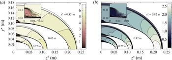
(a) Streamwise Mach number,
 $M_{x}$
, and (b) dimensionless base flow streamwise mass flux,
 $\bar{\unicode[STIX]{x1D70C}}\bar{u}$
, at axial positions
 $x^{\ast }=0.22$
,
 $0.42$
and 0.82 m. The vicinity of the minor-axis meridian at
 $x^{\ast }=0.82~\text{m}$
is shown in detail.

3 Results
3.1 Base flow
The HIFiRE-5 test payload consists of a blunt-nosed elliptic cone of
 $2\,:\,1$
ellipticity and
 $L_{c}^{\ast }=0.86~\text{m}$
length. The nose tip cross-section in the minor axis describes a 2.5 mm radius circular arc, tangent to the cone ray describing the minor axis, and retains a
 $2\,:\,1$
elliptical cross-section to the tip. Flight flow conditions were calculated for a Mach
 $7.45$
flow at an altitude of
 $21.0$
km. The free-stream velocity is
 $\bar{u}_{\infty }^{\ast }=2207.18~\text{m}~\text{s}^{-1}$
, the free-stream temperature is
 $\bar{T}_{\infty }^{\ast }=218.45~\text{K}$
and the corresponding unit Reynolds number is
 $Re^{\prime }=1.015\times 10^{7}~\text{m}^{-1}$
. The surface or wall temperature distribution,
 $\bar{T}_{w}$
, was defined using a prescribed temperature based on heat conduction analysis of an estimated trajectory for the vehicle. The wall temperature near the nose is approximately 650 K and varies between 300 and 400 K over most of the surface of the cone. Downstream of the nose, the ratio between the wall temperature and the corresponding adiabatic wall temperature is
 $\bar{T}_{w}/\bar{T}_{a,w}<0.3$
. More details about the definition of the wall temperature are given by Gosse et al. (Reference Gosse, Kimmel and Johnson2014). The steady laminar flow solution was calculated using the US3D non-equilibrium solver with shock fitting algorithm (Nompelis, Drayna & Candler Reference Nompelis, Drayna and Candler2005) by Gosse et al. (Reference Gosse, Kimmel and Johnson2010) and is used to extract the base flow analysed here at different distances from the cone vertex. High-enthalpy effects were not considered at the present relatively low hypersonic Mach number. The mesh resolution was based on a previous grid resolution study of a sharp elliptic cone and on a study conducted by Choudhari et al. (Reference Choudhari, Chang, Jentink, Li, Berger, Candler and Kimmel2009) and Li et al. (Reference Li, Choudhari, Chang, White, Kimmel, Adamczak, Borg, Stanfield and Smith2012), who both conducted stability analysis of the laminar flow over the HIFiRE-5 vehicle. The grid used was
 $450\times 300\times 300$
(body length by surface normal by radial). A further description of the computation of the base flow as well as some characteristic of its topology are found in Gosse et al. (Reference Gosse, Kimmel and Johnson2010, Reference Gosse, Kimmel and Johnson2014). Furthermore, the authors showed a good qualitative agreement of the calculated heat transfer with experiments conducted in a hypersonic quiet tunnel (Juliano & Schneider Reference Juliano and Schneider2010; Borg et al.
Reference Borg, Kimmel and Stanfield2011) at similar conditions.
Figure 2 shows contours of streamwise Mach number,
 $M_{x}$
, and base flow streamwise mass flux,
 $\bar{\unicode[STIX]{x1D70C}}\bar{u}$
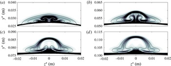
, at different intermediate axial sections of the cone. In the same figure, the stationary mushroom-like vortical structure formed in the vicinity of the minor-axis meridian is shown in detail. The figure shows the spanwise variation of streamwise Mach number and mass flux in the inviscid region between the boundary-layer edge and shock layer. As previously mentioned, the three-dimensional shape of the elliptic cone inevitably produces spanwise pressure gradients, which induce cross-flow, and the flow direction of the interior of the boundary layer is no longer co-planar with the edge velocity vector, unlike circular cones at zero angle of attack. The low-momentum boundary-layer fluid near the surface is deflected from the leading-edge or major-axis meridian towards the minor-axis meridian or centreline. This produces a lift-up of low-momentum boundary-layer fluid at the centreline, generating a low-velocity streak away from the wall, as is observed in figure 3. This figure shows shaded contours of streamwise velocity shear,
 $\bar{u}_{s}=[(\unicode[STIX]{x2202}\bar{u}/\unicode[STIX]{x2202}y)^{2}+(\unicode[STIX]{x2202}\bar{u}/\unicode[STIX]{x2202}z)^{2}]^{1/2}$
, superimposed with contour lines of
 $\bar{u}$
at four different axial positions; namely,
 $x^{\ast }=0.22$
,
 $0.42$
,
 $0.62$
and
 $0.82$
m, which correspond to
 $x/L_{c}=0.26$
,
 $0.49$
,
 $0.72$
and
 $0.95$
, respectively. As the low-velocity streak forms, it induces a three-dimensional detached high-shear layer in its surroundings. A priori, the analysis of such flow structure is only accessible to the present multi-dimensional stability analysis, because classic LST or PSE cannot consider base flows with spanwise gradients of the same order as wall-normal gradients.
Contours of streamwise velocity shear,
 $\bar{u}_{s}$
, showing the localized shear generated at the minor-axis meridian. (a), (b), (c) and (d) correspond to
 $x^{\ast }=0.22$
,
 $0.42$
,
 $0.62$
and 0.82 m, respectively. Solid lines refer to isolines of
 $\bar{u}=0.1:(0.1):0.9$
.

3.2 Instability analysis
The spatial BiGlobal analysis is performed here at a broad range of axial positions and frequencies. As discussed in § 2, the symmetries of the elliptic cone geometry allow the reduction of the discretized domain to one quarter of the cone, using either symmetric or antisymmetric boundary conditions on the major- and minor-axis meridians, as explained in table 1. The symmetric and antisymmetric centreline modes are associated with varicose or sinuous deformations of the low-velocity streak formed in the centreline; they are a consequence of the instability developing in the three-dimensional shear layer. On the opposite side, and at this high-Reynolds-number flow condition, symmetric and antisymmetric high-frequency boundary-layer modes are also amplified in the attachment-line region. Cross-flow and oblique second modes are also observed in the spatial BiGlobal spectrum for low and high frequencies, respectively. The amplitude functions of these modes peak at azimuthal locations along the cone, where the azimuthal variations of the base flow are smaller than wall-normal variations. These modes present an azimuthal sinusoidal shape, which indicates the obliqueness of the instability wave.
3.2.1 Centreline instabilities
The centreline instabilities are obtained using spatial BiGlobal analysis at distances from the cone tip equal to
 $x^{\ast }=0.28$
,
 $0.36$
,
 $0.52$
and 0.72 m, which correspond to
 $x/L_{c}=0.33$
,
 $0.42$
,
 $0.60$
and
 $0.84$
, respectively, and for the broad range of amplified frequencies,
 $F^{\ast }\in (0,550)~\text{kHz}$
. Multiple unstable centreline instability modes are found for each combination of
 $x$
and
 $F$
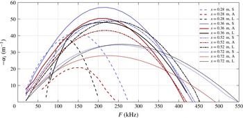
. For simplicity, only the overall most amplified modes are considered next. Figure 4 shows the growth rate of the most amplified centreline modes with symmetric and antisymmetric boundary conditions applied. The symmetric centreline mode is more unstable than the antisymmetric mode for all the
 $x$
positions and frequencies studied. The most amplified frequencies at each axial position for symmetric and antisymmetric modes are similar. Although the range of amplified frequencies is broad, the maximum amplified frequency remains in a narrow band between
 $150$
and 250 kHz along the cone. The maximum growth is achieved at
 $x^{\ast }=0.36~\text{m}$
and
 $F^{\ast }\approx 220~\text{kHz}$
for both symmetric and antisymmetric modes. Although the BiGlobal eigenvalue problem, which does not consider non-parallel effects, is used here, the resulting growth rates can be integrated along the axial positions as solving an spatial initial value problem in a similar way as made in the solution of the PSE-3D analysis (Paredes Reference Paredes2014; Paredes et al.
Reference Paredes, Hanifi, Theofilis and Henningson2015). Doing this, the
 $N$
-factors reach values larger than
 $N=20$
at
 $x^{\ast }=0.72~\text{m}$
for frequencies between 150 and 250 kHz. A
 $N$
-factor of
 $N=20$
means that external perturbations are amplified by a factor of
 $e^{20}\approx 5\times 10^{8}$
, and therefore the transition threshold would be reached even for quiet environmental flight conditions.
Since, to the authors’ knowledge, detailed experiments or direct numerical simulations are not available for the centreline instability problem, the well-known one-dimensional local LST with surface curvature effects is used on the inflectional centreline profile, and results are used as reference values and are included in the same figure 4. LST analysis assumes axisymmetric flow and geometry, neglecting the strong azimuthal variations of the centreline vortical structure. Contrary to expectations, the LST predictions of amplified frequencies and growth rates at each axial position are in fair agreement with the BiGlobal results. The LST results approximate BiGlobal symmetric mode growth rates for increasing axial positions.
Growth rates of leading symmetric (S) and antisymmetric (A) centreline modes computed with the spatial BiGlobal technique. Additionally, growth rates resulting from LST analysis (L) of the profile over the centreline are included.

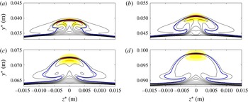
Streamwise velocity magnitude,
 $|\hat{u} |$
, of leading symmetric centreline modes at maximum amplified frequencies for each axial position. Namely, (a)
 $x^{\ast }=0.28~\text{m}$
and
 $F^{\ast }=140~\text{kHz}$
, (b)
 $x^{\ast }=0.36~\text{m}$
and
 $F^{\ast }=220~\text{kHz}$
, (c)
 $x^{\ast }=0.52~\text{m}$
and
 $F^{\ast }=230~\text{kHz}$
and (d)
 $x^{\ast }=0.72~\text{m}$
and
 $F^{\ast }=250~\text{kHz}$
. The colour map varies from
 $|\hat{u} |=0$
(light yellow) to
 $|\hat{u} |=1$
(dark red). The black isolines correspond to
 $\bar{u}=0:(0.1):0.9$
and the thicker blue lines indicate the critical layers.

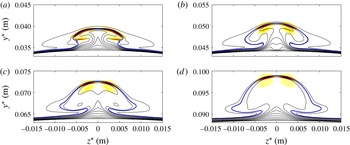
Streamwise velocity magnitude,
 $|\hat{u} |$
, of leading antisymmetric centreline modes at maximum amplified frequencies for each axial position. Namely, (a)
 $x^{\ast }=0.28~\text{m}$
and
 $F^{\ast }=140~\text{kHz}$
, (b)
 $x^{\ast }=0.36~\text{m}$
and
 $F^{\ast }=220~\text{kHz}$
, (c)
 $x^{\ast }=0.52~\text{m}$
and
 $F^{\ast }=220~\text{kHz}$
and (d)
 $x^{\ast }=0.72~\text{m}$
and
 $F^{\ast }=220~\text{kHz}$
. The colour map varies from
 $|\hat{u} |$
=0 (light yellow) to
 $|\hat{u} |=1$
(dark red). The black isolines correspond to
 $\bar{u}=0:(0.1):0.9$
and the thicker blue lines indicate the critical layers.

Several differences are found when comparing these results with the analogous study at a lower Reynolds number,
 $Re^{\prime }=1.89\times 10^{6}~\text{m}^{-1}$
, by Paredes & Theofilis (Reference Paredes and Theofilis2015). In that case, the growth rates of symmetric and antisymmetric modes were almost coincident because the near-centreline instabilities peaked adjacent to the centreline symmetry plane. The amplitude functions of these components decayed to zero at the centreline symmetry plane. The streamwise velocity magnitude of symmetric and antisymmetric centreline modes is plotted in figures 5 and 6, respectively, for the corresponding most amplified frequencies at each axial location. Obeying their physical nature, the shear layer modes peak over the critical layer (
 $\bar{u}=c_{ph}$
, where
 $c_{ph}=\unicode[STIX]{x1D714}/\unicode[STIX]{x1D6FC}_{r}$
is the phase speed of the instability modes). Unlike the lower Reynolds number case of Paredes & Theofilis (Reference Paredes and Theofilis2015), here the maximum value of the amplitude function of the most unstable centreline modes is located at the minor-axis meridian,
 $z=0$
. Also, figure 5 shows how this mode becomes more localized on the wall-normal centreline shear layer at the top of the vortical structure further downstream. A similar observation is found for the antisymmetric modes in figure 6, in which their amplitude functions peak also in the near vicinity of the centreline. In this case, because of the imposed antisymmetric boundary conditions, only the
 ${\hat{w}}$
amplitude function peaks on the centreline. while the rest are zero at the symmetry plane. Amplitude functions of the other components are zero on the symmetry plane. This feature of the antisymmetric modes is a consequence of the imposed centreline boundary conditions, and is distinct from the low-Reynolds-number behaviour of the symmetric and antisymmetric near-centreline modes, which both decayed to zero well away from the centreline.
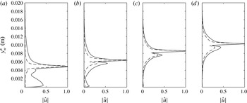
In order to understand the agreement between the LST and BiGlobal predictions of figure 4, the amplitude function of the streamwise velocity component of the most amplified perturbations is plotted in figure 7. Results for LST and BiGlobal analysis are compared. Similar amplitude function profiles are found on the centreline for the four axial locations studied. Again, as in the comparison of growth rate predictions of figure 4, the profiles become more similar as the axial position increases and the amplitude of the BiGlobal eigenfunction becomes more localized on the symmetry plane. It is important to notice that the centreline instabilities are not second Mack mode boundary-layer modes as has been reported in the literature; instead, they correspond to a shear layer or Kelvin–Helmholtz type of instability.
Comparison of normalized streamwise velocity magnitude of centreline symmetric perturbation from spatial BiGlobal analysis (solid line) with the LST mode (dashed line) at the minor-axis meridian for the same frequencies and axial positions as in figure 5, i.e. (a)
 $x^{\ast }=0.28~\text{m}$
and
 $F^{\ast }=140~\text{kHz}$
, (b)
 $x^{\ast }=0.36~\text{m}$
and
 $F^{\ast }=220~\text{kHz}$
, (c)
 $x^{\ast }=0.52~\text{m}$
and
 $F^{\ast }=220~\text{kHz}$
and (d)
 $x^{\ast }=0.72~\text{m}$
and
 $F^{\ast }=220~\text{kHz}$
.

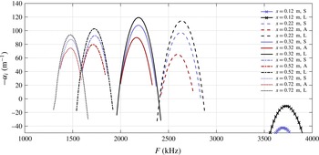
Growth rates of leading symmetric and antisymmetric attachment-line modes. The growth rates resulting from LST analysis on profiles over the major-axis meridian,
 $y=0$
, are added for comparison.

3.2.2 Attachment-line instabilities
Unlike the centreline modes, which have been shown to be driven by the detached high-shear regions of the complex vortical structure formed in the centreline region, attachment-line modes are defined as boundary-layer instabilities. In similarity with the centreline region, the attachment line also exhibits non-negligible variations of the base flow components with respect to the spanwise or azimuthal direction. This occurs mainly on the
 $\unicode[STIX]{x1D701}=0$
symmetry plane, where the streamlines diverge as shown in figure 1. Furthermore, the real surface curvature around the attachment line enhances the three-dimensionality of the flow in this region. Both effects can only be taken into account by the present BiGlobal or two-dimensional stability analysis technique.
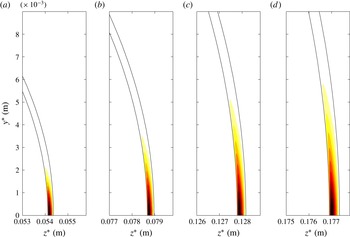
Streamwise velocity magnitude,
 $|\hat{u} |$
, of attachment-line symmetric perturbation at maximum amplified frequency for each
 $x$
positions. Namely, (a)
 $x^{\ast }=0.22~\text{m}$
and
 $F^{\ast }=2620~\text{kHz}$
, (b)
 $x^{\ast }=0.32~\text{m}$
and
 $F^{\ast }=2180~\text{kHz}$
, (c)
 $x^{\ast }=0.52~\text{m}$
and
 $F^{\ast }=1730~\text{kHz}$
and (d)
 $x^{\ast }=0.72~\text{m}$
and
 $F^{\ast }=1480~\text{kHz}$
. The colour map varies from
 $|\hat{u} |=0$
(light yellow) to
 $|\hat{u} |=1$
(dark red). The black isolines correspond to
 $\bar{u}=0$
and
 $0.9$

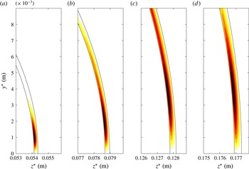
Streamwise velocity magnitude,
 $|\hat{u} |$
, of attachment-line antisymmetric perturbation at maximum amplified frequency for each
 $x$
position. Namely, (a)
 $x^{\ast }=0.22~\text{m}$
and
 $F^{\ast }=2600~\text{kHz}$
, (b)
 $x^{\ast }=0.32~\text{m}$
and
 $F^{\ast }=2160~\text{kHz}$
, (c)
 $x^{\ast }=0.52~\text{m}$
and
 $F^{\ast }=1710~\text{kHz}$
and (d)
 $x^{\ast }=0.72~\text{m}$
and
 $F^{\ast }=1480~\text{kHz}$
. The colour map varies from
 $|\hat{u} |=0$
(light yellow) to
 $|\hat{u} |=1$
(dark red). The black isolines correspond to
 $\bar{u}=0$
and
 $0.9$
.

Attachment-line instabilities are computed using spatial BiGlobal analysis by discretizing a complete
 $(\unicode[STIX]{x1D702},\unicode[STIX]{x1D701})$
-plane from the major-axis,
 $\unicode[STIX]{x1D701}=0$
, to the minor-axis,
 $\unicode[STIX]{x1D701}=\unicode[STIX]{x03C0}/2$
, meridians of the cone, and clustering points towards the wall,
 $\unicode[STIX]{x1D702}=0$
, as explained in § 2.3. Results are shown at distances from the cone tip equal to
 $x^{\ast }=0.12$
,
 $0.22$
,
 $0.32$
,
 $0.52$
and
 $0.72$
m, equal to
 $x^{\ast }=0.28$
,
 $0.36$
,
 $0.52$
and
 $0.72$
m, which correspond to
 $x/L_{c}=0.14$
,
 $0.26$
,
 $0.37$
,
 $0.60$
and
 $0.84$
, respectively, and for the very broad range of amplified frequencies,
 $F^{\ast }\in (0,4000)~\text{kHz}$
. Figure 8 shows the growth rate of the most amplified attachment-line modes with symmetric and antisymmetric boundary conditions. The symmetric mode is more unstable than the antisymmetric mode for all the
 $x$
-positions and frequencies studied. As expected for second Mack modes, the amplified frequency band at each position is narrow and moves towards lower frequencies for increasing
 $x$
-position and the associated increase of the boundary-layer thickness. The frequencies corresponding to maximum growth rates at each axial location are slightly lower for the antisymmetric modes than for the symmetric modes. The narrow amplified frequency band at each axial position translates to a short streamwise amplification domain. Large growth rates are associated with these disturbances. The maximum growth rate observed in figure 8 is
 $-\unicode[STIX]{x1D6FC}_{i}^{\ast }\approx 120~\text{m}^{-1}$
at
 $x^{\ast }=0.32~\text{m}$
. The resulting
 $N$
-factors reach values above
 $N=10$
from
 $x^{\ast }=0.4~\text{m}$
, which is in agreement with the results obtained by Gosse et al. (Reference Gosse, Kimmel and Johnson2014), who solved the PSE analysis along the leading-edge grid line. Confidence in their results is supported by the good prediction given by LST analysis, as shown in figure 8. One-dimensional local LST is used to analyse the boundary-layer profile at the leading edge, similar to the analysis previously performed for the centreline instability case. Results compare favourably with symmetric attachment-line modes. Although LST analysis slightly overpredicts the growth rates, the values of the amplified frequencies are well predicted. The small differences observed between the local LST and BiGlobal growth rates must be due to the real surface curvature and the azimuthal gradients of the base flow variables in this region, which are accounted for only by the BiGlobal analysis.
Figures 9 and 10 show the absolute value of the streamwise velocity of the most amplified attachment-line symmetric and antisymmetric perturbations, respectively. It is observed that the isolines of
 $\bar{u}=0$
and
 $\bar{u}=0.9$
represent the surface wall and the boundary-layer thickness, respectively. The amplitude functions of both symmetric and antisymmetric modes are concentrated inside the boundary layer, as is expected for second Mack mode instabilities (Mack Reference Mack1984). The main difference between symmetric and antisymmetric modes is that all the components but the azimuthal velocity of the symmetric mode peak on the major-axis meridian, while all the components but the azimuthal velocity of the antisymmetric mode are zero at the symmetry plane,
 $\unicode[STIX]{x1D701}=0$
. The different axial stations display a mild modification of these modes downstream. The maxima of the shape functions of these modes are localized in a small azimuthal region near the attachment line. The antisymmetric modes extend farther from the attachment line than the symmetric modes.
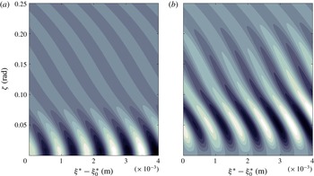
Figure 11 shows the streamwise wave reconstruction of the disturbance density component at the wall,
 $\tilde{\unicode[STIX]{x1D70C}}=\text{Re}(\hat{\unicode[STIX]{x1D70C}}\exp (\text{i}\unicode[STIX]{x1D6FC}(\unicode[STIX]{x1D709}-\unicode[STIX]{x1D709}_{0})))$
. The most amplified symmetric and antisymmetric attachment-line modes at
 $\unicode[STIX]{x1D709}_{0}^{\ast }=x^{\ast }=0.32~\text{m}$
are plotted. Although the base flow and shape functions change along
 $x^{\ast }$
, this variation is negligible for the streamwise range shown in the figure,
 $\unicode[STIX]{x1D709}^{\ast }-\unicode[STIX]{x1D709}_{0}^{\ast }\in (0,0.004)~\text{m}$
. It is observed that both the symmetric and antisymmetric attachment-line modes become oblique for
 $\unicode[STIX]{x1D701}\neq 0$
. Their obliqueness, defined as the angle with respect to the inviscid streamlines, which correspond to grid lines of constant
 $\unicode[STIX]{x1D701}$
, increases for larger
 $\unicode[STIX]{x1D701}$
as the direction of the near-wall streamlines diverge from the inviscid streamlines towards the centreline.
Contours of attachment-line disturbance density component,
 $\tilde{\unicode[STIX]{x1D70C}}$
, at the wall,
 $\unicode[STIX]{x1D702}=0$
, in the vicinity of the attachment line (
 $\unicode[STIX]{x1D701}=0$
) and streamwise coordinate
 $\unicode[STIX]{x1D709}_{0}^{\ast }=x^{\ast }=0.32~\text{m}$
. The disturbance frequencies are (a)
 $F^{\ast }=2180~\text{kHz}$
for symmetric and (b)
 $F^{\ast }=2160~\text{kHz}$
for antisymmetric boundary conditions. The colour map varies from
 $\tilde{\unicode[STIX]{x1D70C}}=-1$
(white) to
 $\tilde{\unicode[STIX]{x1D70C}}=1$
(black).

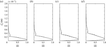
The good agreement between the growth rates predicted by LST and BiGlobal analysis observed in figure 8 is supported by the comparison of the shape functions of the most amplified modes in figure 12. This figure shows the streamwise velocity absolute value profiles at the leading-edge symmetry plane of the same symmetric perturbations shown in figure 9. They are compared with their LST analogues. Both profiles are almost coincident.
Comparison of normalized streamwise velocity magnitude of attachment-line symmetric perturbation from spatial BiGlobal analysis (solid line) with the LST mode (dashed line) at the major-axis meridian for the same frequencies and axial positions as in figure 9.

Contours of oblique second-mode disturbance density component,
 $\tilde{\unicode[STIX]{x1D70C}}$
, at the wall,
 $\unicode[STIX]{x1D702}=0$
, in the vicinity of the attachment line (
 $\unicode[STIX]{x1D701}=0$
) and streamwise coordinate
 $\unicode[STIX]{x1D709}_{0}^{\ast }=x^{\ast }=0.32~\text{m}$
. The disturbance frequency is
 $F^{\ast }=2000~\text{kHz}$
. The colour map varies from
 $\tilde{\unicode[STIX]{x1D70C}}=-1$
(white) to
 $\tilde{\unicode[STIX]{x1D70C}}=1$
(black).

3.2.3 Oblique second modes
Oblique second modes in the HIFiRE-5 elliptic cone model were already found by Paredes & Theofilis (Reference Paredes and Theofilis2015) for a lower Reynolds number
 $Re^{\prime }=1.89\times 10^{6}~\text{m}^{-1}$
. In that work, the authors focused their BiGlobal analysis study on the vicinity of the centreline, where ‘baby’ vortices develop. These vortices produce local strong spanwise gradients and thick boundary layers. Under these circumstances, discrete oblique second modes were observed at frequencies in the range of those of the centreline instabilities. Here, oblique second modes close to the centreline were also observed, but their growth rates were lower than for oblique modes closer to the attachment-line region. For this high-Reynolds-number flow condition,
 $Re^{\prime }=1.015\times 10^{7}~\text{m}^{-1}$
, the most amplified second modes are the previously mentioned attachment-line instabilities. At each axial position, less amplified oblique second modes are found for lower frequencies. In agreement with second Mack mode theory (Mack Reference Mack1984), the frequency of the second modes decreases with increasing boundary-layer thickness. It was observed that by decreasing the frequency, the location of the amplitude function peak moves from the vicinity of the attachment line,
 $\unicode[STIX]{x1D701}=0$
, towards the centreline,
 $\unicode[STIX]{x1D701}=\unicode[STIX]{x03C0}/2$
. Also, the maximum growth rates decrease as frequency decreases. Therefore, the maximum amplified oblique second modes are found in the proximity of the attachment line. An example of these instabilities is shown in figure 13. This mode is found at an axial position
 $x^{\ast }=0.32~\text{m}$
(
 $x/Lc=0.37$
) and frequency
 $F^{\ast }=2000~\text{kHz}$
, which approximately corresponds to the maximum amplified frequency of this mode at this axial position. The growth rate of this instability mode is
 $-\unicode[STIX]{x1D6FC}_{i}^{\ast }=61.27~\text{m}^{-1}$
, which is around a half of the maximum growth rate for the attachment-line instability at the same axial position (see figure 8). The obliqueness of this instability is demonstrated in the same figure 13. Based on the amplitude function shape, the authors think that this particular oblique second mode is a discrete mode, i.e. isolated in the spectrum, because the spanwise characteristic length corresponding to the change of the geometry curvature is of the same order as the spanwise wavelength of this instability. Approximately the same
 $\unicode[STIX]{x1D6FC}$
and
 $\hat{\boldsymbol{q}}$
are recovered for both symmetric and antisymmetric boundary conditions because the amplitude function has already decayed at the symmetry plane,
 $\unicode[STIX]{x1D701}=0$
. Because of the similarities of the oblique second modes with the attachment-line modes, both of which are found to be second Mack instabilities, the attachment-line modes can be identified as the oblique second modes at the leading edge.
3.2.4 Cross-flow instabilities
The cross-flow instabilities are caused by the inflectional three-dimensional boundary-layer profile formed over the surface of the cone between the minor- and major-axis meridians. Therefore, their shape functions are present over most of the surface of the cone. Because of this, large resolutions are needed to solve these modes using the BiGlobal analysis technique. Two resolutions were used to ensure convergence of results,
 $(N_{\unicode[STIX]{x1D701}},N_{\unicode[STIX]{x1D702}})=(601,181)$
and
 $(N_{\unicode[STIX]{x1D701}},N_{\unicode[STIX]{x1D702}})=(1001,221)$
. Although the eigenvalues of the cross-flow branch depend on the resolution, the number of points used was found to be good enough to recover smooth solutions of the cross-flow modes up to a certain wavenumber. The boundary condition imposed at the centreline has a small effect on these modes, although it is not negligible. On the other hand, the boundary condition at the attachment-line boundary has no effect on the eigenvalues and eigenfunctions of the cross-flow modes because the modes vanish towards
 $\unicode[STIX]{x1D701}=0$
. This fact implies that the cross-flow modes are not linked to attachment-line instabilities in this hypersonic flow problem, which is contradictory to what has been observed at the incompressible regime for swept infinite wings (Bertolotti Reference Bertolotti2000). In that incompressible context, these authors found that cross-flow instabilities are fed by their attachment-line counterparts, which is not the case here.
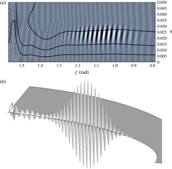
The mode plotted in figure 14 was recovered using symmetric boundary conditions at axial location
 $x^{\ast }=0.32~\text{m}$
(
 $x/L_{c}=0.37$
) and frequency
 $F^{\ast }=60~\text{kHz}$
. Its axial wavenumber is
 $\unicode[STIX]{x1D6FC}_{r}^{\ast }=492.01~\text{m}^{-1}$
and growth rate is
 $-\unicode[STIX]{x1D6FC}_{i}^{\ast }=1.34~\text{m}^{-1}$
. A similar shape was found with antisymmetric boundary conditions. The extension of the shape function up to the centreline explains the observed mild effect of the boundary condition at the centreline,
 $\unicode[STIX]{x1D701}=\unicode[STIX]{x03C0}/2$
. The axial growth rate,
 $-\unicode[STIX]{x1D6FC}_{i}$
, of the cross-flow modes is much smaller than the one associated with the previously listed instabilities. The cross-flow mode shown in figure 14 corresponds to one of the continuous cross-flow branch of modes that appears in the BiGlobal spectrum. Note that the minor-axis centreline is located at the left side of figure 14(a,b). Also, its high obliqueness is clearly visible, which translates into a small azimuthal wavelength. The associated small wavelength together with the mild variation of the base flow with respect to the azimuthal direction, far from the symmetry planes,
 $\unicode[STIX]{x1D701}=0$
and
 $\unicode[STIX]{x1D701}=\unicode[STIX]{x03C0}/2$
, suggests that other more efficient instability analysis techniques could be employed to study these instabilities for this type of flow problem. For example, the quasi-3D or surface-marching PSE (Chang Reference Chang2004; Mughal Reference Mughal2006; Johnson & Candler Reference Johnson and Candler2010) would be a good candidate for this purpose because it includes the effect of mild variations of the base flow variables with respect to both streamwise and spanwise directions.
Cross-flow mode at
 $x^{\ast }=0.32~\text{m}$
and
 $F^{\ast }=60~\text{kHz}$
with symmetric boundary condition. (a) Contours of
 $\text{Re}(\hat{u} )$
in the plane of computational coordinates
 $(\unicode[STIX]{x1D701},\unicode[STIX]{x1D702})$
. The black lines correspond to
 $\bar{u}=0.3$
,
 $0.6$
and
 $0.9$
. (b) Three-dimensional view of
 $\text{Re}(\hat{u} )$
in physical space with axes
 $(z,y,\text{Re}(\hat{u} ))$
. The colour map of part (a) varies from
 $|\hat{u} |=-1$
(white) to
 $|\hat{u} |=1$
(black).

4 Summary and conclusions
A systematic parametric study is presented of the modal global linear instability of boundary-layer flow over the HIFiRE-5 geometry elliptic cone in hypersonic
 $Ma=7.45$
flow at zero angle of attack, a flight altitude of 21.8 km and unit Reynolds number
 $Re^{\prime }=1.015\times 10^{7}~\text{m}^{-1}$
. The analysis is performed using the spatial BiGlobal model, which fully resolves the base flow and its perturbations at selected streamwise locations on planes normal to the cone axis. The parametric study consists of examining the broad range of frequencies from
 $0$
to 4 MHz in order to unravel different types of amplified modal instabilities. Results show that four classes of amplified global eigenmodes exist: (1) centreline modes centred in the shear layer at the minor-axis meridian, (2) attachment-line instabilities in the vicinity of the major axis, as well as (3) cross-flow and (4) oblique second-mode instabilities in the three-dimensional boundary-layer area in between the minor- and major-axis meridians.
Due to the high shear at the minor-axis centreline symmetry plane at this high
 $Re^{\prime }$
, both symmetric and antisymmetric centreline instability modes are amplified in this area. The symmetric mode is found to be more unstable at the studied streamwise positions, reaching
 $N$
-factor values larger than
 $N=20$
from
 $x^{\ast }\approx 0.7~\text{m}$
for frequencies between
 $150$
and 250 kHz. Owing to the localized wall-normal shear over the symmetry plane, classic linear stability analysis, employed upon the one-dimensional profiles at the symmetry plane, is fairly successful in recovering the eigenvalues (streamwise wavenumbers and growth rates) and eigenfunctions (wall-normal profiles). The eigenfunctions are here compared to the wall-normal portion of the two-dimensional eigenfunction of the leading symmetric centreline global mode.
It is worth noting in this context that Juliano et al. (Reference Juliano, Borg and Schneider2015b
) observed transition on HIFiRE-5 at zero angle of attack at
 $Re_{x}=2.8\times 10^{6}$
under quiet flow conditions. In the earlier related work of Paredes & Theofilis (Reference Paredes and Theofilis2015) at a lower unit Reynolds number,
 $Re^{\prime }=1.89\times 10^{6}~\text{m}^{-1}$
, a different modal instability scenario was identified. At those conditions, the highest shear is located adjacent to the centreline flow structure. Consequently, the leading centreline instabilities in those conditions peak over the highest shear regions and vanish towards the plane of symmetry. This relatively lower Reynolds number regime is perhaps more relevant to transition prediction along the centreline, since the rapid growth of centreline instabilities lead to transition at relatively low Reynolds numbers. Under those conditions, classic linear stability theory or PSE, both of which assume lateral homogeneity of the base flow profile, are not expected to yield useful predictions, and use of global instability theory becomes mandatory.
At the attachment line formed near the major-axis meridian, both symmetric and antisymmetric instabilities have been discovered. The symmetric modes are found to be more unstable than their antisymmetric counterparts. Taking into account their instability characteristics, namely, phase velocities close to the slow acoustic speed, high frequencies larger than 1 MHz, and narrow amplified frequency bands at each axial position, it is concluded that the attachment-line instabilities can be catalogued as second Mack modes. Local linear stability theory results also approximate closely the symmetric mode shape function at the plane of symmetry and predict well the range of amplified frequencies, although growth rates are slightly overestimated by the classic analysis.
Spatial BiGlobal instability analysis has been used here for the first time to study the boundary-layer modes amplified over the surface of the cone between the leading edge and centreline. At low frequencies, stationary and travelling cross-flow instabilities have been recovered. Cross-flow modes away from the attachment line appear to be distinct from the attachment-line instabilities. Cross-flow instabilities are present on most of the surface but vanish towards the attachment line. This contrasts with the experience with swept infinite wings at the incompressible limit (Bertolotti Reference Bertolotti2000) and the related swept cylinder problem in supersonic flow (Mack, Schmid & Sesterhenn Reference Mack, Schmid and Sesterhenn2008). In these cases, the attachment-line instabilities in the leading-edge region connected with cross-flow modes further away from the attachment line.
Oblique second Mack modes are also amplified along the surface of the cone. Their growth rates decrease as the modes peak farther from the leading-edge symmetry plane. Close to the leading edge, the oblique second modes have a frequency slightly below those of attachment-line instabilities, but are much less amplified, e.g. the growth rate of the most unstable oblique second mode at
 $x^{\ast }=0.32~\text{m}$
is nearly half of the growth rate corresponding to the symmetric attachment-line mode at the same axial location.
Overall, at the conditions examined, the centreline modes are the strongest candidates to lead to transition. Such an assertion has to be verified by additional analysis work employing PSE-3D, which has been shown to predict linear (De Tullio et al. Reference De Tullio, Paredes, Sandham and Theofilis2013) and nonlinear (Paredes et al. Reference Paredes, Hanifi, Theofilis and Henningson2015) direct numerical simulation results at a much lower level of computing effort compared with DNS. At the same time, PSE-3D can also address flow instability at non-zero angles of attack and yaw, and thus yield predictions for additional flight regimes of the elliptic cone. Work is underway to address these issues, and results will be reported in due course.
Acknowledgements
Fruitful discussions with Dr H. L. Reed are gratefully acknowledged. This effort is sponsored by the Air Force Office of Scientific Research, Air Force Material Command, USAF, under grant no. FA8655-12-1-2004. The US Government is authorized to reproduce and distribute reprints for Governmental purpose notwithstanding any copyright notation thereon. DISTRIBUTION A. Approved for public release: distribution unlimited. 88ABW-2015-5929, 09 Dec 2015.