1. Introduction
Policy-makers and observers are increasingly concerned about the economy's ability to generate, and keep up with, a pace of technological progress capable of fostering economic growth. At its highest institutional level, the European Union has made explicit – with the 2000 Lisbon Strategy for Growth and Jobs – its objective of promoting innovation and its diffusion. According to the European Commission ‘productivity growth require[s] a continued investment in a highly skilled and adaptable workforce. Economies endowed with a skilled labor force are better able to create and make effective use of new technologies.’Footnote 1 Recently, reforms of public financing schemes for research have been implemented (e.g. in Great Britain, Germany, and France) and the average length of higher education curricula is increasing (e.g. in Spain, Italy, and France). There is a clear public concern for providing the economy with a high supply of skilled workers able to effectively perform research and development (R&D) tasks or to adapt to and adopt new technologies. This skill scarcity within the European Union is perceived as a major constraint on its competitiveness.
A related concern is raised by commentators in the US. The dependence of the national research system on the supply of researchers from abroad became noticeable following the fall of the Berlin wall and the visa restrictions in the aftermath of the terrorist attacks of 2001. The inflow of foreign graduate students affects the academic research sector, with spillovers on private R&D. The instability of this flow, and its unpredictability, are sources of public concern. Some observers suggest that the national system of higher education should provide a larger and steadier supply of graduate students and researchers, as a strategy to ensure the sustainability of US technological leadership (Romer, Reference Romer2000).
On the one hand, the level and scope of this debate demonstrate an increasing political awareness of the scarcity of human resources necessary to sustain a continuous and rapid pace of technological change and economic growth. On the other hand, well-established wisdom in natural resource economics suggests that overcoming the constraint imposed by the scarcity of natural resources on future production requires appropriate investment in R&D targeted at resource-augmenting technological progress (e.g. Aghion and Howitt, Reference Aghion and Howitt1998: ch. 5; Amigues et al., Reference Amigues, Grimaud and Moreaux2004a; Amigues et al., Reference Amigues, Long and Moreaux2004b; Tsur and Zemel, Reference Tsur and Zemel2005). We therefore raise the question of whether and to what extent the scarcity of human resources available to perform R&D can frustrate society's ability to face up to the constraint imposed by natural resource scarcity. In this paper we set up a theoretical framework to shed some light on this – previously unexplored – double scarcity problem.
A two-sector growth model with an essential non-renewable natural resource is presented. We perform a normative analysis of the strategies of resource exploitation and labor allocation between two possible tasks: production and R&D. This paper builds on previous work by Amigues et al. (Reference Amigues, Grimaud and Moreaux2004a), Amigues et al. (Reference Amigues, Long and Moreaux2004b), and Amigues and Moreaux (Reference Amigues and Moreaux2004). A Leontief technology is assumed for the production of the consumption good, which uses labor and the natural resource. We suppose that R&D activity uses labor to improve the efficiency of a unit of natural resource in the production of the consumption good. Resource-augmenting technological progress is endogenous and effective, because its potential contribution to production is unbounded.Footnote 2 Here we extend these previous analyses to examine how the heterogeneity of the labor force affects optimal paths.
If skills differ across individuals, we need to establish an efficient way to assign individuals to the competing tasks of production and R&D. In the next section we deal with this issue. We allow the differentiation of individuals according to two dimensions: their absolute productivity in each sector and their relative productivity, i.e. they can be ranked in terms of their comparative advantage in performing production tasks versus R&D task.Footnote 3 Efficient allocation implies assigning individuals to tasks according to their position in the comparative advantage ranking. Using this rule, we define the set of maximum feasible combinations of effective labor input in production and in R&D as the effective labor possibilities frontier of the economy (ELPF). This frontier summarizes information concerning the size of the labor force and the distribution of skills across it, reflecting, importantly, the correlation of absolute sector-specific productivity across individuals. We find that, as long as individuals are differentiated in their relative productivity, the opportunity cost of R&D in terms of foregone production is an increasing function of the level of R&D activity. In fact, as the R&D sector expands it needs to employ workers with ever lower comparative advantage in R&D. This opportunity cost is greater if the ranking based on comparative advantage coincides with the one based on absolute advantage, since in this case R&D employees can be hired out of the least productive workers. This case prevails if individuals have specialized skills. Otherwise, i.e. in the case of weak skill specialization, individuals may be highly differentiated in absolute productivity but poorly so in relative productivity. Then the opportunity cost of R&D is not very elastic. The shape of the ELPF specifies precisely this trade-off, since its slope is an index of the opportunity cost of R&D.
In section 3 we set up the normative problem and study the dynamics of the system, including the properties of the optimal steady state and transition paths. We find that the ELPF plays a crucial role in determining the socially optimal trajectory of the economy, but that it is not significant in the long run (i.e. the optimal steady state is similar to that found assuming that labor is perfectly substitutable between production and R&D, see Amigues et al., Reference Amigues, Grimaud and Moreaux2004a). In order to illustrate our finding, consider the case when initially the economy is endowed with low natural resource stock. We show that it is optimal to maintain resource-augmenting technical progress during the transition above its steady state rate. In order to do this, more workers will be assigned to R&D tasks during transition, only to be gradually released to the production sector at a later date. Increasing R&D employment, however, requires reducing employment in production, and therefore depressing consumption. The greater is the opportunity cost of R&D in terms of consumption, the more interesting it becomes to spread out the R&D plan over time, by initially employing less researchers–engineers but for a longer period of time. As a consequence, the greater is this opportunity cost, i.e. the more concave is the ELPF, the slower is the period of transition. We find that if labor is heterogeneous in such a way that individual skills are relatively specialized, it is optimal to perform relatively little R&D, targeted at substituting the scarce natural resource, and letting the transition phase be relatively slow. The inverse can be said in the case of a resource-scarce economy endowed with a flexible labor force, where labor is relatively homogeneous, i.e. not greatly differentiated in relative productivity.
In view of the importance played by the distribution of relative skills across the active population, we may consider the opportunity of modifying this distribution. In section 4 we provide a taxonomy of three types of possible shifts of the ELPF. In each case we perform comparative statics exercises and discuss possible intertemporal trade-offs. We also present examples of changes in population distribution underpinning the shift of the ELPF. In doing so, we discuss important policy issues, such as education policies and demographic evolutions.
Several papers are related to ours. From a methodological point of view, our approach is to be contrasted with the seminal work on the possibility and social desirability of investing in physical capital to substitute for exhaustible resources (see Dasgupta and Heal, Reference Dasgupta and Heal1979, for a synthesis of the early literature). We neither allow for capital accumulation, nor for the substitution of other inputs for the scarce resource. We consider instead the accumulation of technical knowledge, which can substitute for the resource. A notable difference is that in our case, potential accumulation is unbounded, since R&D does not require – directly or indirectly – natural resource inputs (see Groth, Reference Groth2007). Endogenous growth theory based on intentional investment in resource-augmenting R&D has been used to explore similar issues. Smulders and de Nooji (Reference Smulders and de Nooij2003) and Van Zon and Yetkiner (Reference Van Zon and Yetkiner2003) consider cases with an exogenous evolution of the price of the natural resource, constant in the former and exogenously increasing in the latter. Instead Aghion and Howitt (Reference Aghion and Howitt1998: ch. 5), Scholz and Ziemes (Reference Scholz and Ziemes1999), Schou (Reference Schou2000), Grimaud and Rouge (Reference Grimaud and Rouge2003) allow for an endogenous determination of resource prices. All these papers only consider the case of homogeneous workers, when labor is perfectly substitutable between production and R&D and the ELPF is linear.
There is a strand of literature that deals more explicitly with the process of development of resource substitutes and/or reduction in resource extraction cost. The early approach assumed the discrete introduction of backstop technologies (Dasgupta et al., Reference Dasgupta, Heal, Majumdar and Intriligator1977; Davison, Reference Davison1978; Kamien and Schwartz, Reference Kamien and Schwartz1978). More recently Tahvonen and Salo (Reference Tahvonen and Salo2001) and Tsur and Zemel (Reference Tsur and Zemel2005) consider cases of endogenous and continuous processes. The former, however, rely on the assumption of unintentional technological progress (i.e. learning-by-doing). Tsur and Zemel explicitly consider the R&D effort and show, as we do, that relatively resource-poor economies have relatively strong incentives to engage in R&D activity. In contrast to us, they find that only economies initially endowed with a sufficiently large amount of physical capital and technological knowledge can afford R&D programs ambitious enough to sustain a growing (constant in our framework) consumption path.Footnote 4
Finally, this paper is related to macroeconomic dynamic analyses that assume some form of adjustment costs. It is possible to draw a parallel between this line of literature and our model with regard to the result concerning the influence of the ELPF shape on optimal transition speed. We do this at some length at the end of section 3. Here it is worthwhile noticing that the ELPF is closer to the ‘intratemporal’ adjustment costs proposed by Huffman and Wynne (Reference Huffman and Wynne1999) than to alternative specifications in the literature. However, while Huffman and Wynne simply assume the existence of a concave frontier to shift new capital (or labor) from one sector to the other, we derive the analogous frontier and prove its concavity from first-order assumptions concerning only the heterogeneity of individual skills within the population. Moreover, we do not assume any real cost of reallocating workers between sectors, differently from Bertola (Reference Bertola1994), who assumes that firms incur firing and hiring costs, or Krugman (Reference Krugman1991), who posits a quadratic ‘moving cost’ function à la Mussa (Reference Mussa1978). It should be emphasized that the ELPF and its derivation in section 2 constitute an original theory of adjustment costs based only on the plausible assumption of the heterogeneity of individual skills.
2. The effective labor possibilities frontier
We distinguish between three levels of labor input. First, ‘raw’ units of labor, which are hours of work supplied, determined exogenously by population size. Second, ‘effective’ units of labor supplied in each sector, which, as shown in this section, depend on the distribution of individuals over the space of productivity bundles and on the allocation of workers to sectors. Third, ‘efficiency’ units of labor supplied in each sector, which may vary across time as a result of dedicated R&D activity, i.e. even if the allocation of effective units of labor is constant. This third distinction will play a role in our analysis from the next section onward.
An individual is characterized by a vector measuring his or her productivity in each of the different tasks to which he or she can be assigned. In R&D-based growth models, including ours, there are typically two sectors – production and R&D – and this vector is two-dimensional. An individual denoted by index i is characterized by how many instantaneous units of effective labor he or she can supply to the production sector, denoted by λi, and how many instantaneous units of effective labor he or she can instead supply to the R&D sector with one unit of raw labor, denoted by νi. The vector {νi, λi} summarizes the skills of individual i. We assume that, at a given date, each individual must specialize and work in one sector only.Footnote 5 Nevertheless, it is assumed that a continuum of – possibly different – agents exists and that the reallocation of workers across sectors or of one individual over time does not entail any direct cost.
At any given date, we denote by P the total mass of individuals in the economy, by λ and ν the highest sector-specific skills present within the population, and by  (ν, λ) the population density on the skill bundle {ν, λ} in the domain of feasible skill bundles Γ ≡ {ν, λ|ν ∈ [0, ν], λ ∈ [0, λ]} ⊂ ℜ+2, hereafter called the ‘skills space’. By definition population size is P = ∫0ν ∫0λ (ν, λ)dλ dν. The aggregate amount of effective labor in R&D is denoted by n. Its maximum value is obtained by allocating all individuals to this task, which yields ∫0ν ∫0λ (ν, λ)ν dλ dν ≡ n. Similarly, aggregate effective labor input to production, denoted by l, is always constrained to be smaller than or equal to ∫0λ ∫0ν (ν, λ)λ dν dλ ≡ l.
To each allocation of individuals to tasks corresponds a bundle of effective labor inputs in the (n, l) space. The aim of the present analysis is to establish the efficient way of allocating individuals to tasks. Given the amount of effective labor provided to the R&D sector, efficiency prescribes that effective units of labor in production cannot be increased simply by reallocating workers across tasks. We introduce the effective labor possibilities frontier as follows:
Definition 1. The effective labor possibilities frontier (ELPF)  : [0, n] → [0, l] is the function associating the maximum effective units of labor (n) that can be employed in production with every feasible level of effective units of labor in R&D n.
The following proposition characterizes the building process of the ELPF.
Proposition 1. The ELPF is obtained by allocating individuals to tasks according to their comparative advantage.
Proof. We show in section 1 of the appendixFootnote 6 that, starting from the efficient allocation of workers described in proposition 1, any reallocation of workers implies a loss of l if n is held constant.□
Each individual i∈[0, P] is characterized by an index of relative skill for production θi≡λi/νi. Relatively low values of θ signify a comparative advantage in R&D, and higher θs stand for a comparative advantage in production. The rule of efficient allocation is the following: for any given n, choose θ high enough so that precisely n effective units of labor are supplied to R&D if all the individuals i such that {νi,  (θνi)}, where (θνi) ∈ [0, min{θνi, λ}), are assigned to R&D, while all individuals j characterized by {νj, λ(θνj)}, where λ(θνj) ∈ (min{θνj, λ} λ], perform production tasks. This procedure defines a threshold
 (n) on the scale of relative skill indices, such that all individuals with θi < (n) are assigned to R&D to supply n effective units of labor inputs, and all individuals with θj > (n) are employed in production.
Adopting this allocation rule, we can draw the ELPF by varying θ between 0, for which n = 0 and l = l, and ∞, for which n = n and l = 0. For θ < θ ≡ l/n the amount of efficiency units of labor provided to R&D is computed by considering that there is a mass ∫0θν (ν, λ)dλ of individuals with R&D skill ν allocated to R&D tasks, each supplying ν efficiency units of labor, so that n 1(θ) = ∫0ν ν(∫0θν (ν, λ)dλ)dν is an increasing function of θ. To compute the efficiency units of labor provided to production for θ < θ, we sum the contribution of individuals characterized by production skills λ <  ≡ν, which according to the previous reasoning give
 , and the contribution of those with skills λ > , all of whom are assigned to production. This gives
 , i.e. a decreasing function of θ.Footnote 7 Mutatis mutandis, for θ > θ there exists
 = λ/θ such that the allocation rule defines the maximum amount of efficiency units of labor that can be supplied to each sector as follows
 and l 2(θ) = ∫0λ λ(∫0λ/θ (ν, λ)dν)dλ. To summarize

with ∂ñ(θ)/∂θ > 0 and ∂ (θ)/∂θ < 0. Hence, the ELPF is defined by substituting for θ in (θ) using the inverse function θ = ñ −1(n)

Proposition 2. The ELPF is decreasing. It is linear if individuals are characterized by the same relative skill index θ≡λ/ν and it is quasi-concave in every other case. It is strictly concave if population density is positive on a continuous interval of relative skill indices:

Proof. See section 2 of the appendix (see footnote 6). The frontier is decreasing because increasing effective labor inputs in one sector requires a reduction in raw labor inputs in the other sector, and the productivity of raw labor is never negative. To prove the quasi-concavity of the ELPF we first obtain its explicit expression in the case of a one-point mass distribution to show that it is linear with slope θ. Then we obtain the expression for the case of a two-point mass distribution and show that the ELPF is linear if and only if the two points lie on the same ray (i.e. are characterized by the same θ), and that it is piecewise linear quasi-concave in every other case. Finally, any population distribution that is continuous on some subset of Γ is equivalent to the union of an infinite number of one-point distributions. If the subset of Γ does not coincide with the ray, the θ characteristic of each one-point distribution varies continuously so that the ELPF is the envelope of an infinite number of piecewise linear quasi-concave functions, i.e. it is a strictly concave function. □
The common assumption employed in the literature on growth theory (e.g. Romer, Reference Romer1990; Aghion and Howitt, Reference Aghion and Howitt1992; Jones, Reference Jones1995a) and natural resources economics (e.g. Aghion and Howitt, Reference Aghion and Howitt1998: ch. 5; Scholz and Ziemes, Reference Scholz and Ziemes1999; Amigues et al., Reference Amigues, Grimaud and Moreaux2004a) is that of a linear ELPF since labor is assumed to be homogenous.
Proposition 2 establishes that the ELPF cannot be a convex function. A comparison with a canonical production possibilities frontier (PPF) may help in understanding the result. In standard microeconomics textbooks, the PPF defines efficient combinations of goods that can be produced employing some homogeneous raw input (e.g. raw labor) according to a set of given technologies (i.e. production functions). The PPF can be a convex function if the underlying technologies are characterized by sufficiently strong increasing returns to scale (e.g. if a production function is linear and the other convex). In building the ELPF, as an intermediate step and by analogy to the production function, we can define the ‘ranking’ functions n = kn(N) and l = kl(L) associating every feasible value of raw labor inputs to each sector, N, L∈[0, P], with the efficient level of sector-specific effective units of labor. The shape of the ranking functions depend, on the one hand, on population distribution over the skills space – given exogenously – and, on the other, on the allocation of individuals to tasks – an endogenous process. This endogeneity implies that the two ranking functions depend on each other, differently from the production functions in the canonical PPF model. For instance, if kn(N) is linear, then kl(L) must also be linear, since individuals are not differentiated in their comparative advantage. Conversely, if kn(N) is convex, reflecting an increasing average productivity (n/N) of researchers–engineers, then kl(L) is strongly concave, since decreasing raw labor inputs are matched with falling average productivity (l/L). The interdependence of ranking functions prevents the ELPF from being convex.Footnote 8 Heterogeneity of individual skills implies a large scope for convexifying the economy production possibility set, as discussed toward the end of the next section.
Let us now explain which factors determine the degree of concavity of the ELPF. The slope of this frontier measures the opportunity cost of supplying a marginal effective unit of labor to R&D in terms of forgone effective labor inputs to production. As the units of effective labor supplied to the R&D sector expand, this opportunity cost may increase. Whether or not this happens, and to what extent it does, depends on the population distribution over the skills space and in particular on the correlation of skills across individuals. If the most productive researchers–engineers are also the most skilled workers in production, the correlation of skills is positive and thus the ELPF is relatively flat.Footnote 9 The frontier is in fact linear in the case of perfect (unit) correlation.Footnote 10 Concavity of the frontier increases as the correlation of skills across individuals approaches minus one. In the case of a negative correlation in fact, increasing effective labor in R&D by one unit requires reallocating ever more raw labor out of production and into R&D since ever-less effective researchers–engineers are employed, so that their average productivity falls.Footnote 11
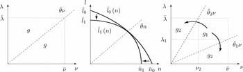
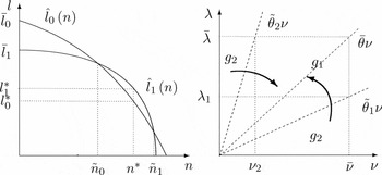
The following examples show how the correlation of skills across individuals determines the degree of concavity of the ELPF. Consider first the case of a uniform distribution of individuals over the skills space, i.e. (ν, λ) = g > 0 ∀ {ν, λ} ∈ Γ (see the left-hand-side panel of figure 1). This case corresponds to a unimodal distribution of population around θ. In section 3.1 of the appendix we compute the ELPF and obtain the following continuous envelope of two concave functionsFootnote 12

Correlation of skills across individuals and shape of the ELPF

Let us next modify the population distribution into a heterogeneous one, characterized by a stronger negative correlation of individual skills. We do this by moving individuals located close to the relative skill index θ toward the extremes of the support. This experiment exacerbates differences in comparative advantage.Footnote 13 We define two thresholds  1 ∈ (0, θ) and 2 ∈ (θ, ∞), then reduce population density to g 1 < g in the area between the two rays 1 ν and 2 ν, and increase population density in the rest of Γg 2 < g just enough to keep the same population size (see the right-hand-side panel of figure 1). This defines λ1 = 1ν and ν2 = λ/2. The ELPF is then the envelope of four concave functionsFootnote 14

This frontier is more concave than the one obtained for a uniform population distribution (1), and more concave the greater is the heterogeneity within the distribution, i.e. the larger g − g 1 and g 2 − g. The middle-panel of figure 1 represents the two ELPFs when all other parameters are identical and the s are symmetric. In this case 1(n) is strictly interior to the set defined by the frontier 0(n) prevailing for uniform distribution, and the frontiers coincide only when the labor-allocation threshold is at its critical level θ. In all other cases the gain obtained by having more specialized individuals is outweighed by the loss due to the lower availability of adaptable workers. The loss is greater the more polarized is employment, i.e. the closer we moves to the axes along the ELPF.
3. Optimal resource extraction and R&D investment paths
In this section, we carry out the normative analysis of the paths of resource extraction, labor allocation, and R&D effort. First we explicitly set up the objective of the social planner and we introduce assumptions concerning production possibilities, including the role of natural resources. Next we derive the necessary and sufficient conditions for solving the social planner's problem. These are used to perform the analysis of the optimal dynamic behavior of the economy. To this end, we study the qualitative features of the steady state and of transition.Footnote 15
We consider an economy in which population and its distribution over the skills space are constant over time.Footnote 16 We assume that individuals supply labor inelastically and normalize population size (i.e. total raw labor supply) to unity.
Our normative approach relies on the assumption that a benevolent social planner seeks to maximize welfare, defined as the sum of instantaneous isoelastic utilities, generated by a stream of consumption c ≡ {ct}∞0 and discounted at some constant rate ρ

The economy can produce some Hicksian consumption good, denoted yt, from effective labor, lt, and a non-renewable natural resource. Let st be the resource input measured in physical units. The efficiency of each production factor depends upon specific technical knowledge. For simplicity, we assume that only the resource efficiency index can be improved through dedicated research effort. Let A be the constant efficiency index of effective labor inputs and Bt the efficiency index of resource use at time t. Inputs measured in efficiency units are then Alt and Btst, which are assumed to be strict complements. The production function is

This Leontief production function is extreme in making the efficiency units of natural resource an essential input. Of course knowledge, as measured by Bt, can substitute for physical resource inputs. This specification allows us to distinguish clearly the role played by production versus R&D activity. An efficient use of inputs requires that

The research sector employs nt units of effective labor inputs. Its output is expressed in terms of growth rate of the resource productivity index Bt

with b > 0. This assumption can also be interpreted as saying that the stock of current technical knowledge, measured by Bt, enters as a (non-rival) factor with constant returns to scale in the production of new technology, i.e. the flow Ḃ t.Footnote 17
Combining (4), (5), and ct ≤ yt to restrict attention to efficient paths, we have

In this formulation the double scarcity problem is clearly put forward. Natural resource scarcity (low st) has ceteris paribus a depressive impact on consumption. Only technological improvement (increasing Bt) can balance this effect.Footnote 18 Promoting technological progress requires reallocating labor toward R&D and out of production (low lt), which in turn tends to depress (current) consumption.
The social planner's problem may be formulated as a problem with only one control variable and two state variables. We choose the formulation in which the control variable is nt. Using (3)–(7), the program is

First let us note that ∀t ct > 0 since  , hence lt > 0 and n − n t ≥ 0, implying that st > 0, hence Ṡ t < 0. Deleting these constraints, we write the Lagrangian of the problem as follows

Functions μ and ω are costate variables for the stock of physical resource and for the level of efficiency index, respectively. The γ s are multipliers for the non-negativity constraint on R&D employment. The first-order condition is

together with the complementary slackness condition γn,t ≥ 0 and γn,tnt = 0. We assume γn,t = 0 to restrict attention to trajectories with active R&D. The dynamics of the costate variables μt and ωt must satisfy


and the transversality conditions at infinity

These conditions imply limt→∞ S t = 0 and limt→∞ ωt = 0 since the resource has a positive value μ > 0, and the stock of knowledge is non-decreasing.Footnote 19 Moreover, the values of the two stocks should always be equalizedFootnote 20

In the aftermath of the analysis we use the following definitions and notations:
Definition 2. Effective resource stock: Rt ≡ BtSt.
Definition 3. Elasticity of the ELPF:
 .
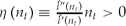
Definition 4. Elasticity of the opportunity cost of R&D:
.Definition 5. The function X(R t, n t) ≡ R t/[A
′(n t)] < 0.
 .
 .
The dynamics of the system is characterized by the way one control, n, and one state variable, R, evolve, according to


These differential equations are obtained in the analysis presented in section 4 of the appendix (see footnote 6). From (14) at the steady state, we have R* = A (n*)/bn*, which, using the definitions of X and σ, implies that

For the numerator of the right-hand side of (15) to be zero at the steady state, the following must hold

substituting (16) for X* in this expression and using previous results, we obtain:
Proposition 3. There exists an optimal steady state if and only if

in which case the constant endogenous variables are equal to

According to Proposition 3, at the steady state the key variable ruling the dynamics of the system, R&D employment, is independent of the shape of the ELPF, which instead affects the levels of consumption and effective resource stock at the steady state, through its level effect, i.e. to what extent steady state R&D employment determines the level of effective labor in production via the exogenous relationship (ρ/b).
The result according to which R&D effort is an increasing function of the rate of preference for the present was already found by Amigues et al. (Reference Amigues, Grimaud and Moreaux2004a). R&D activity entails the accumulation of resource-augmenting technological knowledge. It therefore constitutes a form of saving. According to (18) a relatively impatient society optimally saves more (and consumes less). This result may appear puzzling but actually reflects feasibility constraints. In order to maintain a steady flow of consumption, a constant flow of resource inputs in efficiency units is required. At the steady state, the flow of extracted resources in physical units declines at the same rate as stock of natural resources, i.e. at rate ρ (the Hotelling rule). As a result, it is necessary to increase the efficiency of natural resource inputs at that same rate. R&D employment must be set at n* to obtain Ḃ/B = ρ and keep the effective stock of resource, R, constant. In a relatively impatient society, it is efficient to deplete the physical stock of natural resources at a faster rate. This requires assigning relatively more workers to R&D to cope with increasing natural resource scarcity.
The dynamics of the system outside the steady state are characterized by the following:
Proposition 4. The steady state is the unique saddle path stable equilibrium. Along the stable arms:
• if R 0 < R*, R&D activity is relatively high (i.e. n > n*) and falling over time, consumption is relatively low (i.e. c < c*) and increasing during the transition;Footnote 21
• if R 0 > R*, R&D activity is relatively low (i.e. n < n*) and increasing over time, consumption is relatively high (i.e. c > c*) and falling.Footnote 22
Proof. The phase diagram of system (14)–(15) in the (R, n) space is characterized by the Ṙ = 0 locus being decreasing from n down to zero asymptotically, with R falling below this schedule and increasing above it, and by the ṅ = 0 locus increasing, with n falling above this schedule and increasing below it. The saddle path leading to the steady state lies above the Ṙ = 0 schedule for R 0 < R* and vice versa. For the detailed proof and illustration, please see section 4 of the appendix (see footnote 6). □
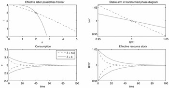
The flexibility in labor allocation plays a role in the short and medium term. What was not visible under the assumption of a linear ELPF (e.g. in Amigues et al., Reference Amigues, Grimaud and Moreaux2004a; Amigues et al., Reference Amigues, Long and Moreaux2004b) is that the law of motion of the R&D employment n, equation (15), depends on both σ(n) and η(n), which measure the concavity of the frontier. The transition toward the steady state depends upon the shape of the ELPF because the slope of the latter provides a measure of the opportunity cost of R&D in terms of forgone (potential) output. To exemplify this result, we run simulations of the transition period, and compare the results obtained for frontiers with varying degrees of concavity but holding the steady state level of consumption constant. We perform comparative dynamics exercises only for the purpose of exploring the qualitative features of the model. We use the following functional form for the ELPF

Hence, (0) = l, (n) = 0,  ,
 implying the restriction δ > 1 for coherence with proposition 2. We have chosen this specification because it provides an easy way to modify the concavity of the frontier, by changing δ.Footnote 23 Under this specification, the elasticity of the ELPF is variable and equal to σ = δ(n/n)δ/[1 − (n/n)δ], while the elasticity of the opportunity cost of R&D is constant and equal to η = δ − 1. Given the qualitative aim of our analysis, the values of parameters, other than ɛ, are not important because they imply only scale shifts (if condition (17) is satisfied). For the baseline case presented here, parameters' values are set at ρ = .2, l = 4, n = 4, b = .1, A = 1. The intertemporal elasticity of substitution influences the socially optimal investment policy, as it is extensively explained in Amigues and Moreaux (Reference Amigues and Moreaux2004). For this critical parameter, we have chosen the common value ϵ = 1.5. To perform comparative dynamics we vary the value of δ. Moreover, we limit the comparison to economies that reach the same steady state level of per capita consumption. To ensure this we adjust n.Footnote 24
Figure 2 reports results for economies that are more flexible (with low δ = 4/3, dashed line) and less flexible (with high δ = 4, continuous line). In the north-west panel the ELPF are represented, with circles indicating the steady state employment bundle. The relatively flexible economy (dashed ELPF) is characterized by a lower opportunity cost of R&D in terms of forgone inputs to production. It follows that in the transition phase the flexible economy performs relatively more R&D if it needs to accumulate effective resources, and less R&D if it is endowed with too many. This can be seen from the stable arm in the phase diagram depicted in the north-east panel of figure 2: for any given negative deviation of the stock of effective resource from its steady state value, R&D is more distant from its long term level in the more flexible economy, and vice versa. As a consequence, transition to the steady state is much faster in the more flexible economy. In the example illustrated in the south-east panel, the more flexible economy takes about half the time the less flexible economy needs to eliminate the gap in effective resource stock. To start off with the same level of effective resources and reach the steady state more quickly, requires a relatively greater effort in R&D during transition. All this translates into relatively rapid change in consumption, i.e. higher growth rate of per capita consumption in an economy accumulating effective resources.Footnote 25
Comparison of transitions

We conclude that the scarcity of skills in R&D plays an important role in shaping the possibilities for the economy to cope with the scarcity of natural resources during transition. Since we have formalized the scarcity of R&D inputs as a problem of flexibility in the allocation of the labor force, scarcity is significant when the system is undergoing change, so that labor needs to be reallocated across sectors.
A remarkable implication of this result on the role of the frontier for the transition is that the framework introduced in this paper provides an original theory of (implicit) adjustment costs in the literature on dynamic macroeconomic modeling, namely in R&D-based growth theory. We can in fact draw a parallel with the existing literature on adjustment costs to highlight similarities and differences with our analysis. In the standard Ramsey–Cass–Koopmans (RCK) model of growth, the aggregate accumulation constraint, Y = c +  , implies a linear production possibilities frontier in the (, c) space.Footnote 26 The optimal steady state is represented by a single bundle on this PPF. In the RCK model, adjustment costs can be introduced by assuming a convex function for the instantaneous cost of investment, I() with I′, I″ > 0.Footnote 27 In this case, the accumulation constraint, Y = c + I(), implies a concave PPF in the , c) plane. The more concave is the PPF, the slower is transition to the steady state (see e.g. Abel, Reference Abel1982). Abstracting from the natural resource constraint, we can define a PPF for our model in the Ḃ/B, c) space. Given that technologies (4) and (6) are linear, the PPF is linear if the ELPF is linear, i.e. if labor is homogenous in relative skills (as in Amigues et al., Reference Amigues, Grimaud and Moreaux2004a; Amigues et al., Reference Amigues, Long and Moreaux2004b). Conversely, the PPF is concave if the ELPF is concave, i.e. if labor is heterogeneous in relative skills. Moreover, the degree of concavity of the PPF is entirely determined by that of the ELPF.Footnote 28 It is therefore possible to argue that heterogeneity in skills across workers implies a form of adjustment cost. Similarly to macroeconomic models using adjustment costs (e.g. Mussa, Reference Mussa1978; Turnovsky, Reference Turnovsky1996), we find that the degree of concavity of the ELPF – hence of the PPF – counts for the speed of transition.Footnote 29 The major difference lies in the origin of the concavity of the PPF. Differently from the previous approaches we do not assume any direct instantaneous cost of reallocating factors across tasks, and in so doing we avoid introducing technological assumptions that directly imply the concavity of the efficiency frontier.Footnote 30 It is noteworthy that in our case its concavity is due, on the one hand, to the plausible assumption of heterogeneity of skills across individuals and, on the other, to the efficient allocation of these individuals to tasks, which is a result and not an assumption of the analysis. In other words we identify an original justification for adjustment costs, one that is micro-founded and exclusively based on opportunity costs.Footnote 31
4. Policy analysis
In the previous sections, we have built and used a model to analyze the socially optimal paths of resource extraction and targeted R&D activity for a given distribution of population over the skills space. In this section we study the consequences of modifications in this distribution, particularly with regard to the shape of the ELPF. These modifications may be the result of intentional policies, such as education policy, or of structural changes, such as demographic evolutions.
Although we allow for modifications in population distribution, we make no assumption on timing and costs, i.e. we do not specify technologies that shift the ELPF. Modelling these technologies would take us far beyond the scope of this paper.Footnote 32 We would rather restrict our attention to shifts of the ELPF that implicitly model a trade-off, i.e. that include some cost.Footnote 33 In the rest of this section we distinguish between three different types of shift of the ELPF. In each case we give examples of modifications in the population distribution over the skills space that generates the shift. This comparative dynamics exercise allows us to identify policies that characteristically imply the type of shift of the frontier.Footnote 34 Admittedly a single policy may imply changes encompassing more than one of the three types of shift that we have identified.
4.1. Demographic expansion
A first type of modification in the population distribution is the one that implies an homothetic outward shift of the ELPF. This is for instance the consequence of a skill-neutral demographic expansion, i.e. a uniform increase in population density over the skills space.Footnote 35 Such a shift in the ELPF increases the potential effective labor inputs that can be employed in any sector. There is however a cost associated with this improvement in possibilities: since B 0 and S 0 are given, there are initially less per capita effective resources available. How does the optimal steady state change?
In section 5 of the appendix (see footnote 6), we provide a detailed answer to this question under the assumption that the social planner is interested in welfare of the representative agent. We find that the steady state level of units of effective labor inputs in R&D is independent of population size (i.e. n* = ρ/b whatever P), and that the steady state level of per capita consumption is an increasing function of population size. Of course for a given amount of initial effective resource stock, a larger population implies lower per capita consumption at the beginning of the transition period. There is a trade-off between initial and steady state per capita consumption.
The positive long-run effect of demographic expansion on per capita consumption may seem surprising in a resource constrained economy. This result depends on three crucial assumptions. First knowledge is a perfect substitute for natural resources, all that matters being the effective stock of resource Rt = BtSt. Second, knowledge accumulation rests on a steady flow of effective labor input in R&D, whose opportunity cost falls with the size of the labor force. This is due to the presence of a scale effect in aggregate R&D, well-known in growth theory (see Jones, Reference Jones1995b; Young, Reference Young1998; Li, Reference Li2000). Third, heterogeneity across workers implies a sort of ‘skill deepening’ effect, an original feature of our analysis, resulting from changes in average productivity of raw labor employed in each sector.
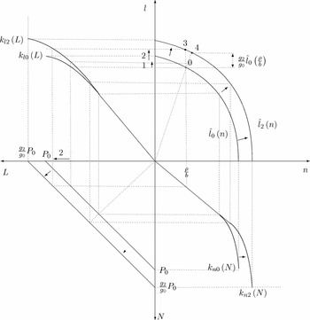
To illustrate these effects, let us assume a uniform population distribution over the constant skills space Γ. Adapting the ELPF as given by expression (1) obtained in the first example of section 2, we see that the ELPF goes through (n = 0, l = P λ/2), (n = P ν/3, l = P λ/3), and n = P ν/2, l = 0), so that changes in P produce homothetic shifts of the frontier. To obtain the ranking functions, we first compute raw labor employed in a sector as a function of θ, under efficient labor allocation (see Proposition 1). We get for θ < θ N = gθν2/2, L = g λν − gθν2/2, and for θ > θ N = g λν − g λ2/(2θ), L = g λ2/(2θ). Combining these results with those on n(θ) and l(θ) developed in section 3.1 of the appendix (see footnote 6), we obtain

and

which are quasi-concave monotonically increasing functions. We denote the ELPFs by 0(n) and 2(n) respectively before and after the demographic expansion. Let us suppose that n* = ρ/b < g 0λν2/3 for the initial level of g 0. If population density increases to g 2 > g 0, so does population size, P = g 2λν, and the raw labor constraint in the south-west panel of figure 3 shifts outwards by the factor g 2/g 0. The ranking functions shift upwards for values of raw labor beyond the threshold g 0λν/2, as illustrated in the north-west and south-east panels of figure 3. The increase in effective units of labor supplied by a given amount of raw labor is due to the ‘skill-deepening’ effect. It implies that the average productivity of raw labor in production (l/L) increases since, holding raw labor inputs constant at L 0, the composition of the sectoral labor force is skewed towards individuals with higher comparative advantage in production.Footnote 36 In figure 3 this ‘skill deepening’ effect is represented by the arrow labeled 1. In the long run, effective labor input in R&D is unchanged at n* = ρ/b. Since population density is higher, a smaller share of the labor force needs to be employed in the R&D sector, that is a smaller labor-allocation threshold θ* is used at the steady state. As a consequence, raw labor is reallocated from R&D to production, further increasing steady state aggregate production and per capita consumption. This is the ‘scale effect’ illustrated by arrows labeled 2 in figure 3. Overall effective labor in production shifts upwards from point 0 to point 3, i.e. from 0(ρ/b) to 2(ρ/b), while an expansion proportional to that of population size – leaving per capita consumption constant – is represented by the vertical distance between points 0 and 4, i.e. (g 2/g 0)0(ρ/b).
A demographic expansion.

4.2. Higher education versus vocational training
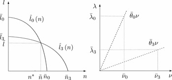
A second type of shift of the ELPF is the case illustrated in figure 4, where the frontier shifts from 0(n) to 3(n) on the pivotal bundle (ñ, ), with 0(ñ) = 3(ñ) = . A shift of this type expands the potential bundles with relatively high effective labor inputs in R&D (on the south-east of the pivotal bundle), at the expense of some previously feasible bundles with relatively high effective labor input in production (on the north-west of the pivotal bundle). To the extent that more effective labor inputs to R&D are feasible and that the frontier is flatter over a large range, the economy can converge more rapidly to its steady state if it is characterized by 3(n) rather than by 0(n) provided they are identical in every other respect and start from an insufficient resource base (R 0 < R*).Footnote 37 This is true even in the case where ñ > n*, i.e. the case in which the steady state level of effective labor inputs in production and per capita consumption are higher in the slower economy than in the faster one, since 0(ρ/b) > 3(ρ/b). In this case, the possibility of (irreversibly) shifting the ELPF from 0(n) to 3(n) implies an intertemporal trade-off.
From vocational training to higher education.

What kind of policies imply this type of shift of the frontier? We use an example to show that this type of shift results from a change in the population distribution over the skills space that (i) reduces the population density of individuals characterized by high productivity in production and low productivity in R&D, (ii) leaves the density unchanged for individuals that have low productivity in both sectors, and (iii) increases (from zero in the example) the density of individuals characterized by high productivity in R&D and low productivity in the production sector. Consider for instance the ELPF as given by expression (1) of section 2 prevailing for a uniform distribution of population over the skills space. The initial distribution is characterized by the threshold θ0 = λ0/ν0. Suppose now that it is possible to move the population distribution to another uniform one with the same density g but over a different skills space characterized by θ3 = λ3/ν3 < θ0 (see the right-hand-panel of figure 4). Same population density and size imply that ν0 < ν3 and λ3 < λ0. The ELPFs are obtained by adding sub-indices to ν and λ to (1). It is trivial that n 3 > n 0 and l 3 < l 0. The pivotal bundle is ñ = g λ3ν02/3.Footnote 38 In the symmetric case when ν0/ν3 = λ3/λ0 and ν3 = λ0 the two ELPFs are perfectly symmetrical (case illustrated in figure 4).
Policies promoting higher education at the expense of vocational training may give rise to this kind of modification of the population density. Easier access to higher education and more difficult access to vocational training might possibly modify the productivity bundles of would-be best production workers and make them become instead the best researchers–engineers. Higher education affects the specialization of (treated) individuals. At the same time improved access to higher education, and worsened access to quality vocational training, would not affect the productivity of individuals with relatively low productivity in both sectors (those in the rectangle delimited by the axes, ν0 and λ3) because of the selective nature of higher education, which only affects the productivity of a part of the population.
4.3. General versus specialized education
A third type of modification of the ELPF concerns its degree of concavity. As explained toward the end of section 2, a low degree of concavity of the frontier corresponds to a relatively flexible labor force, with individual workers characterized by similar relative productivity indices (i.e. the case of high positive correlation of skills across individuals). This is ceteris paribus a desirable feature of the ELPF because the more flexible is the labor force the faster is the transition toward the steady state. Since we do not specify the technology for modifying the shape of the ELPF, we consider the case where the cost associated with greater flexibility takes the form of a lower level of per capita consumption in the long run.
As an example let us compare the case with a uniform population distribution, resulting in the ELPF given by expression (1), with the case where population density is more polarized on the extremes of the relative skill indices, resulting in the ELPF given by expression (2). Situations in which 1(n) dominates 0(n) over some range arise only if the specialization is asymmetric (i.e. if ν2/ν ≠ λ1/λ) or is accompanied by an extension of the distribution over the skills space (i.e. higher ν and/or λ). For instance the case illustrated on the left-hand-side panel of figure 5 prevails when ν2/ν < λ1/λ and the bundle (ν, λ) is unchanged. Here the long-run cost of increasing labor flexibility is represented by lower per capita consumption since n* ∈ (ñ 0, ñ 1), with ñ 0 < ñ 1 defined by 0(ñ 0) = 1(ñ0) and 0(ñ 1) = 1(ñ 1), implies 1(n*) > 0(n*). In this case moving from the specialized distribution, underlying 1(n), to the more uniform one, underlying 0(n), implies skewing rightwards the population distribution over the space of relative skill indices θ, from a distribution relatively concentrated on comparative advantage in R&D (i.e. low θs) to a distribution relatively concentrated around θ. Since the optimal steady state level of effective labor inputs in R&D is unchanged, but a lower density of individuals with comparative advantage in R&D is available, the share of raw labor that is to be assigned to R&D must be larger in the case of the uniform distribution as compared to the case of the heterogeneous distribution concentrated on low values of θ. For this reason there is a loss in the level of consumption.
From specialized to general education.

In the European Union, increasing the flexibility of workers, as well as improving their ability to adapt to and skillfully perform different tasks, is considered a major goal of training and education policy. Among other targets, this policy aims at increasing the generational share of high-school and university graduates, because graduates are seen as more adaptable workers. Raising attainment rates in secondary and tertiary education may be achieved (at least partially) by lowering requirements for attaining diplomas. In this case, the other side of the ‘increased labor adaptability’ coin might be the poorer quality of education received by the most promising students (i.e. those who in any case are educated). The cost of providing general education to a larger number of potential students is given by the lower skills acquired by the best students in each field of specialization (for a given length of curricula). This trade-off is analogous to the case considered above when the density of population over the space of relative productivity indices θ is increased around θ and reduced for lower and for higher values of θ, giving rise to a shift of the frontier from the relatively concave 1(n) to the more flexible 0(n).
5. Conclusion
The simple fact that workers are heterogeneous in their sector-specific productivity implies that, in an efficient economy, the opportunity cost of R&D activity in terms of forgone inputs to production increases with the level of R&D activity. We have introduced the concept of effective labor possibilities frontier to characterize precisely this trade-off. Our first result establishes that the frontier is concave or quasi-concave, apart from the special case of a population where individuals are not differentiated in their comparative advantage (the only case considered so far in the literature). The shape of the frontier is significant for the optimal transition toward the steady state, but not for characterizing the R&D effort in the long run. For example, an economy endowed with relatively scarce natural resources, which needs much resource-augmenting technical progress during transition to cope with resource scarcity, initially performs relatively more R&D the less concave is its frontier. This is the case of a relatively flexible economy, since the opportunity cost of R&D does not change much with the share of the sector in the economy. This second original finding can be interpreted as the result of an adaptation of investment theory with adjustment costs to the case of a two-sector growth model with resource-targeted R&D. Nevertheless, it should be emphasized that the theory that we developed in this paper provides an original micro-foundation of adjustment costs in two-sector growth models. From this point of view, the novelty of our approach lies in its reasonable requirement, i.e. that workers be heterogeneous in their relative skill, which we think is quite plausible. This constitutes a third contribution of the paper.
We have also performed some comparative static exercises to illustrate how the ELPF can be used as a tool for policy analysis. In particular, it has been shown that changes in the population distribution over the skills space imply shifts of the frontier. We provide a taxonomy of possible shifts and give examples of underlying modifications in such distribution. This methodological clarification is another contribution of the paper. When considering real-world cases, our framework suggests a method to distinguish among factors that have different implications. For example, the policies that have recently been adopted in several EU countries, aimed at increasing higher education attainment rates by making curricula longer, imply both a modification of individual skill bundles, similar to the one studied in section 4.2, and a shrinking of (active) population density over the skills space as a consequence of the reduction in the labor force participation rate, similar to (the inverse of) the case considered in section 4.1.Footnote 39 Overall it is shown that the ELPF represents a fruitful, and relatively easy to handle tool to perform policy experiments in previously unexplored, but quite topical, issues.
 ,
 ,
 ,
 , and
 . For the details concerning this case we invite the reader to see section 3.2 in the appendix (see footnote 6).