3.1. Processing of verticality cues

Processing of cues arising from the vertical dimension is a faculty possessed by members of most phyla, and it takes many forms. One of the simplest is detection of the vertical axis itself, using a variety of mechanisms that mostly rely on gravity, or on cues related to gravity, such as hydrostatic pressure or light gradients. This information provides a potential orienting cue which is useful not only in static situations but also for navigation in three-dimensional space. Additionally, within the vertical dimension itself gravity differentiates down from up and thus polarizes the vertical axis. Consequently, animals are always oriented relative to this axis, even though they can become disoriented relative to the horizontal axes. The importance of the gravity signal as an orienting cue is evident in reduced or zero-gravity environments, which appear to be highly disorienting for humans: Astronauts report difficulty in orienting themselves in three-dimensional space when floating in an unfamiliar orientation (Oman Reference Oman, Mast and Jancke2007).

The vertical axis, once determined, can then be used as a reference frame for the encoding of metric information in the domains of both direction and distance. The technical terms for dynamic rotations relative to the vertical axis are pitch, roll, and yaw, corresponding to rotations in the sagittal, coronal, and horizontal planes, respectively (Fig. 2A). Note that there is potential for confusion, as these rotational terms tend to be used in an egocentric (body-centered) frame of reference, in which the planes of rotation move with the subject. The static terms used to describe the resulting orientation (or attitude) of the subject are elevation, bank, and azimuth (Fig. 2B), which respectively describe: (1) the angle that the front-back (antero-posterior) axis of the subject makes with earth-horizontal (elevation); (2) the angle that the transverse axis of the subject makes with earth-horizontal (bank); and (3) the angle that the antero-posterior axis of the subject makes with some reference direction, usually geographical North (azimuth). Tilt is the angle between the dorso-ventral cranial axis and the gravitational vertical.

Figure 2.

(a) Terminolog y describing rotations in the three cardinal planes. (b) Terminology describi ng static orientation (or “attitude”) in each of the three planes.

The other metric category, in addition to direction, is distance, which in the vertical dimension is called height – or (more precisely) elevation, when it refers to distance from a reference plane (e.g., ground or water level) in an upward direction, and depth when it refers to distance in a downward direction. Determination of elevation/depth is a special case of the general problem of odometry (distance-measuring).

There is scant information about the extent to which animals encode information about elevation. A potential source of such information could be studies of aquatic animals, which are exposed to particularly salient cues from the vertical dimension due to the hydrostatic pressure gradient. Many fish are able to detect this gradient via their swim bladders, which are air-filled sacs that can be inflated or deflated to allow the fish to maintain neutral buoyancy. Holbrook and Burt de Perera (Reference Holbrook and Burt de Perera2011a) have argued that changes in vertical position would also, for a constant gas volume, change the pressure in the bladder and thus provide a potential signal for relative change in height. Whether fish can actually use this information for vertical self-localization remains to be determined, however.

The energy costs of moving vertically in water also add navigationally relevant information. These costs can vary across species (Webber et al. Reference Webber, Aitken and O'Dor2000); hence, one might expect that the vertical dimension would be more salient in some aquatic animals than in others. Thermal gradients, which are larger in the vertical dimension, could also provide extra information concerning depth, as well as imposing differential energetic costs in maintaining thermal homeostasis at different depths (Brill et al. Reference Brill, Lutcavage, Metzger, Stallings, Bushnell, Arendt, Lucy, Watson and Foley2012; Carey Reference Carey1992).

Interestingly, although fish can process information about depth, Holbrook and Burt de Perera (Reference Holbrook and Burt de Perera2009) found that they appear to separate this from the processing of horizontal information. Whereas banded tetras learned the vertical and horizontal components of a trajectory equally quickly, the fish tended to use the two components independently, suggesting a separation either during learning, storage, or recall, or at the time of use of the information. When the two dimensions were in conflict, the fish preferred the vertical dimension (Fig. 3), possibly due to the hydrostatic pressure gradient.

Figure 3.

The experiment by Holbrook and Burt de Perera (Reference Holbrook and Burt de Perera2009). (a) Line diagram of the choice maze (taken from the original article, with permission), in which fish were released into a tunnel and had to choose one of the exit arms to obtain a reward. (b) The conflict experiment of that study, in which the fish were trained with the arms at an angle, so that one arm pointed up and to the left and the other arm pointed down and to the right. During testing, the arms were rotated about the axis of the entrance tunnel so that one arm had the same vertical orientation but a different left-right position, and one had the same horizontal (left-right) position but a different vertical level. (c) Analysis of the choices showed that the fish greatly preferred the arm having the same vertical level. Redrawn from the original.

Several behavioural studies support the use of elevation information in judging the vertical position of a goal. For instance, rufous hummingbirds can distinguish flowers on the basis of their relative heights above ground (Henderson et al. Reference Henderson, Hurly and Healy2001; Reference Henderson, Hurly and Healy2006), and stingless bees can communicate the elevation as well as the distance and direction to a food source (Nieh & Roubik Reference Nieh and Roubik1998; Nieh et al. Reference Nieh, Contrera and Nogueira-Neto2003). Interestingly, honeybees do not appear to communicate elevation (Dacke & Srinivasan Reference Dacke and Srinivasan2007; Esch & Burns Reference Esch and Burns1995). Rats are also able to use elevation information in goal localization, and – like the fish in the Holbrook and Burt de Perera (Reference Holbrook and Burt de Perera2009) study – appear to separate horizontal and vertical components when they do so. For example, Grobéty & Schenk (Reference Grobéty and Schenk1992a) found that in a lattice maze (Fig. 4A), rats learned to locate the elevation of a food item more quickly than they learned its horizontal coordinates, suggesting that elevation may provide an additional, more salient spatial cue, perhaps because of its added energy cost, or because of arousal/anxiety.

Figure 4.

Rodent studies of vertical processing. (a) Schematic of the lattice maze of Grobéty and Schenk (Reference Grobéty and Schenk1992a), together with a close-up photograph of a rat in the maze (inset). (b) Schematic and photograph of the pegboard maze used in the experiments of Jovalekic et al. (Reference Jovalekic, Hayman, Becares, Reid, Thomas, Wilson and Jeffery2011) and, as described later, by Hayman et al. (Reference Hayman, Verriotis, Jovalekic, Fenton and Jeffery2011). In the Jovalekic et al. experiment, rats learned to shuttle directly back and forth between start and goal locations, as indicated in the diagram on the right. On test trials, a barrier (black bar) was inserted across the usual route, forcing the rats to detour. The great majority of rats preferred the routes indicated by the arrows, which had the horizontal leg first and the vertical leg second.

Jovalekic et al. (Reference Jovalekic, Hayman, Becares, Reid, Thomas, Wilson and Jeffery2011) also found a vertical/horizontal processing separation in rats, but in the opposite direction from Grobéty and Schenk, suggesting a task dependence on how processing is undertaken. Rats were trained on a vertical climbing wall (studded with protruding pegs to provide footholds; Fig. 4B) to shuttle back and forth between a start and goal location. When a barrier was inserted into the maze, to force a detour, the rats overwhelmingly preferred, in both directions, the route in which the horizontal leg occurred first and the vertical leg second. Likewise, on a three-dimensional lattice similar to the one used by Grobéty and Schenk, the rats preferred the shallow-steep route to the steep-shallow route around a barrier. However, the task in Jovalekic et al.'s study differed from that faced by Grobéty and Schenk's rats in that in the latter, both the starting location and the goal were well learned by the time the obstacle was introduced. It may be that elevation potentiates initial learning, but that in a well-learned situation the animals prefer to solve the horizontal component first, perhaps due to an inclination to delay the more costly part of a journey.

Humans can estimate their own elevation, but with only a modest degree of accuracy. Garling et al. (Reference Garling, Anders, Lindberg and Arce1990) found that subjects were able to judge, from memory, which one of pairs of familiar landmarks in their hometown has a higher elevation, indicating that information about elevation is both observed and stored in the brain. It is not clear how this information was acquired, although there were suggestions that the process may be based partly on encoding heuristics, such as encoding the steepest and therefore most salient portions of routes first, as opposed to encoding precise metric information. Notwithstanding the salience of the vertical dimension, processing of the vertical dimension in humans appears poor (Montello & Pick Reference Montello and Pick1993; Pick & Rieser Reference Pick, Rieser and Potegal1982; Tlauka et al. Reference Tlauka, Wilson, Adams, Souter and Young2007).

As with the fish and rodent studies above, a dissociation between vertical and horizontal processing was seen in a human study, in which landmarks arranged in a 3-by-3 grid within a building were grouped by most participants into (vertical) column representations, and by fewer participants into (horizontal) row representations (Büchner et al. Reference Büchner, Hölscher, Strube, Vosniadou, Kayser and Protopapas2007). Most participants' navigation strategies were consistent with their mental representations; as a result, when locating the given target landmark, a greater proportion of participants chose a horizontal-vertical route. The authors suggested that these results might have been reversed in a building that was taller than it was wide, unlike the building in their study. However, given the results from the rats of Jovalekic et al. (Reference Jovalekic, Hayman, Becares, Reid, Thomas, Wilson and Jeffery2011), in which the climbing wall dimensions were equal, it is also possible that this behaviour reflects an innate preference for horizontal-first routes.

In conclusion, then, studies of both human and nonhuman animals find that there is clear evidence of the use of elevation information in spatial computations, and also for differential processing of information from vertical versus horizontal dimensions. The processing differences between the two dimensions may result from differential experience, differential costs associated with the respective dimensions, or differences in how these dimensions are encoded neurally.

Next, we turn to the issue of how the change in height with respect to change in distance – that is, the slope of the terrain – may be used in spatial cognition and navigation. This is a more complex computation than simple elevation, but its value lies in the potential for adding energy and effort to the utility calculations of a journey.

3.2. Navigation on a sloping surface

Surfaces extending into the vertical dimension locally form either slopes or vertical surfaces, and globally form undulating or crevassed terrain. Slopes have the potential to provide several kinds of information to a navigating animal (Restat et al. Reference Restat, Steck, Mochnatzki and Mallot2004), acting, for instance, as a landmark (e.g., a hill visible from a distance) or as a local organizing feature of the environment providing directional information. Additionally, as described earlier, the added vertical component afforded by slopes is both salient and costly, as upward locomotion requires greater effort than horizontal locomotion, and an extremely steep slope could be hazardous to traverse. As a result, it is reasonable to assume that slopes might influence navigation in several ways.

A number of invertebrates, including desert ants and fiddler crabs, appear able to detect slopes, sometimes with a high degree of accuracy (at least 12 degrees for the desert ant; Wintergerst & Ronacher Reference Wintergerst and Ronacher2012). It is still unknown how these animals perform their slope detection, which in the ant does not appear to rely on energy consumption (Schäfer & Wehner Reference Schäfer and Wehner1993), sky polarization cues (Hess et al. Reference Hess, Koch and Ronacher2009), or proprioceptive cues from joint angles (Seidl & Wehner Reference Seidl and Wehner2008). The degree to which slope is used in ant navigation has been under considerable investigation in recent years, making use of the ability of these animals to “home” (find their way back to the nest) using a process known as path integration (see Etienne & Jeffery Reference Etienne and Jeffery2004; Walls & Layne Reference Walls and Layne2009; Wehner Reference Wehner2003) in which position is constantly updated during an excursion away from a starting point such as a nest.

Foraging ants will home after finding food, and the direction and distance of their return journey provide a convenient readout of the homing vector operative at the start of this journey. Wohlgemuth et al. (Reference Wohlgemuth, Ronacher and Wehner2001) investigated homing in desert ants and found that they could compensate for undulating terrain traversed on an outbound journey by homing, across flat terrain, the horizontally equivalent distance back to the nest, indicating that they had processed the undulations and could extract the corresponding ground distance. Likewise, fiddler crabs searched for their home burrows at the appropriate ground distance as opposed to the actual travelled distance (Walls & Layne Reference Walls and Layne2009). Whether such encoding of slope is relative to earth-horizontal (i.e., the plane defined by gravity) or whether it simply relates the two surfaces (the undulating outbound one and the flat return one), remains to be determined. However, despite the ability of Cataglyphis to extract ground distance, Grah et al. (Reference Grah, Wehner and Ronacher2007) found that the ants did not appear to encode specific aspects of the undulating trajectory in their representations of the journey, as ants trained on outbound sloping surfaces will select homing routes that have slopes even when these are inappropriate (e.g., if the two outbound slopes had cancelled out, leaving the ant at the same elevation as the nest with no need to ascend or descend). Thus, ants do not appear to incorporate elevation into their route memory; their internal maps seem essentially flat.

The ability of humans to estimate the slope of surfaces has been the subject of considerable investigation. Gibson and Cornsweet (Reference Gibson and Cornsweet1952) noted that geographical slant, which is the angle a sloping surface makes with the horizontal plane, is to be distinguished from optical slant, which is the angle the surface makes with the gaze direction. This is important because a surface appears to an observer to possess a relatively constant slope regardless of viewing distance, even though the angle the slope makes with the eye changes (Fig. 5A). The observer must somehow be able to compensate for the varying gaze angle in order to maintain perceptual slope constancy, presumably by using information about the angle of the head and eyes with respect to the body. However, despite perceptual slope constancy, perceptual slope accuracy is highly impaired – people tend to greatly overestimate the steepness of hills (Kammann Reference Kammann1967), typically judging a 5-degree hill to be 20 degrees, and a 30-degree hill to be almost 60 degrees (Proffitt et al. Reference Proffitt, Bhalla, Gossweiler and Midgett1995).

Figure 5.

Visual slant estimation. (a) Slope constancy: A subject viewing a horizonta l surface with a shallow gaze (β₁) versus a steep gaze (β₂) perceives the slope of the ground to be the same (i.e., zero) in both cases despite the optical slant (β) being different in the two cases. In order to maintain constant slope perception, the nervous system must therefore have some mechanism of compensating for gaze angle. (b) The scale expansion hypothesis: An observer misperceives both the declination of gaze and changes in optical slant with a gain of 1.5, so that all angles are exaggerated but constancy of (exaggerated) slant is locally maintained. Increasing distance compression along the line of sight additionally contributes to slant exaggeration (Li & Durgin Reference Li and Durgin2010).

This mis-estimation of slope has been linked to the well-established tendency of people to underestimate depth in the direction of gaze (Loomis et al. Reference Loomis, Da Silva, Fujita and Fukusima1992): If subjects perceive distances along the line of sight to be foreshortened, then they would perceive the horizontal component of the slope to be less than it really is for a given vertical distance, and thus the gradient to be steeper than it is. However, this explanation fails to account for why subjects looking downhill also perceive the hill as too steep (Proffitt et al. Reference Proffitt, Bhalla, Gossweiler and Midgett1995). Furthermore, if observers step back from the edge of a downward slope, there is a failure of slope constancy as well as accuracy: they see the slope as steeper than they do if they are positioned right at the edge (Li & Durgin Reference Li and Durgin2009). Durgin and Li have suggested that all these perceptual distortions can collectively be explained by so-called scale expansion (Durgin & Li Reference Durgin and Li2011; Li & Durgin Reference Li and Durgin2010) – the tendency to overestimate angles (both gaze declination and optical slant) in central vision by a factor of about 1.5 (Fig. 5B). While this expansion may be beneficial for processing efficiency, it raises questions about how such distortions may affect navigational accuracy.

Other, nonvisual distortions of slope perception may occur, as well. Proffitt and colleagues have suggested that there is an effect on slope perception of action-related factors, such as whether people are wearing a heavy backpack or are otherwise fatigued, or are elderly (Bhalla & Proffitt Reference Bhalla and Proffitt1999); whether the subject is at the top or bottom of the hill (Stefanucci et al. Reference Stefanucci, Proffitt, Banton and Epstein2005); and their level of anxiety (Stefanucci et al. Reference Stefanucci, Proffitt, Clore and Parekh2008) or mood (Riener et al. Reference Riener, Stefanucci, Proffitt and Clore2011) or even level of social support (Schnall et al. Reference Schnall, Harber, Stefanucci and Proffitt2012). However, the interpretation of many of these observations has been challenged (Durgin et al. Reference Durgin, Klein, Spiegel, Strawser and Williams2012).

Creem and Proffitt (Reference Creem and Proffitt1998; Reference Creem and Proffitt2001) have argued that visuomotor perceptions of slope are dissociable from explicit awareness. By this account, slope perception comprises two components: an accurate and stable visuomotor representation and an inaccurate and malleable conscious representation. This may be why subjects who appear to have misperceived slopes according to their verbal reports nevertheless tailor their actions to them appropriately. Durgin et al. (Reference Durgin, Hajnal, Li, Tonge and Stigliani2011) have challenged this view, suggesting that experimental probes of visuomotor perception are themselves inaccurate. The question of whether there are two parallel systems for slope perception therefore remains open.

How does slope perception affect navigation? One mechanism appears to be by potentiating spatial learning. For example, tilting some of the arms in radial arm mazes improves performance in working memory tasks in rats (Brown & Lesniak-Karpiak Reference Brown and Lesniak-Karpiak1993; Grobéty & Schenk Reference Grobéty and Schenk1992b; Figure 6a). Similarly, experiments in rodents involving conical hills emerging from a flat arena that rats navigated in darkness found that the presence of the slopes facilitated learning and accuracy during navigation (Moghaddam et al. Reference Moghaddam, Kaminsky, Zahalka and Bures1996; Fig. 6B). In these experiments, steeper slopes enhanced navigation to a greater extent than did shallower slopes. Pigeons walking in a tilted arena were able to use the 20-degree slope to locate a goal corner; furthermore, they preferred to use slope information when slope and geometry cues were placed in conflict (Nardi & Bingman Reference Nardi and Bingman2009b; Nardi et al. Reference Nardi, Nitsch and Bingman2010). In these examples, it is likely that slope provided compass-like directional information, as well as acting as a local landmark with which to distinguish between locations in an environment.

Figure 6.

Behavioural studies of the use of slope cues in navigation, in rats (a and b) and in humans (c). (a) Schematic of the tilted-arm radial maze of Grobéty & Schenk (Reference Grobéty and Schenk1992b). (b) Schematic of the conical-hill arena of Moghaddam et al. (Reference Moghaddam, Kaminsky, Zahalka and Bures1996). (c) The virtual-reality sloping-town study of Restat et al. (Reference Restat, Steck, Mochnatzki and Mallot2004) and Steck et al. (Reference Steck, Mochnatzki, Mallot, Freksa, Brauer, Habel and Wender2003), taken from Steck et al. (Reference Steck, Mochnatzki, Mallot, Freksa, Brauer, Habel and Wender2003) with permission.

In humans, similar results were reported in a virtual reality task in which participants using a bicycle simulator navigated within a virtual town with eight locations (Restat et al. Reference Restat, Steck, Mochnatzki and Mallot2004; Steck et al. Reference Steck, Mochnatzki, Mallot, Freksa, Brauer, Habel and Wender2003; Fig. 6C). Participants experiencing the sloped version of the virtual town (4-degree slant) made fewer pointing and navigation errors than did those experiencing the flat version. This indicates that humans can also use slope to orient with greater accuracy – although, interestingly, this appears to be more true for males than for females (Nardi et al. Reference Nardi, Newcombe and Shipley2011). When slope and geometric cues were placed in conflict, geometric information was evaluated as more relevant (Kelly Reference Kelly2011). This is the opposite of the finding reported in pigeons discussed above. There are, of course, a number of reasons why pigeons and humans may differ in their navigational strategies, but one possibility is that different strategies are applied by animals that habitually travel through volumetric space rather than travel over a surface, in which geometric cues are arguably more salient.

The presence of sloping terrain adds complexity to the navigational calculations required in order to minimize energy expenditure. A study investigating the ability of human participants to find the shortest routes linking multiple destinations (the so-called travelling salesman problem, or “TSP”) in natural settings that were either flat or undulating found that total distance travelled was shorter in the flat condition (Phillips & Layton Reference Phillips and Layton2009). This was perhaps because in the undulating terrain, participants avoided straight-line trajectories in order to minimize hill climbing, and in so doing increased travel distance. However, it is not known to what extent they minimized energy expenditure. Interestingly, Grobéty & Schenk (Reference Grobéty and Schenk1992a) found that rats on the vertical plane made a far greater number of horizontal movements, partly because they made vertical translations by moving in a stair pattern rather than directly up or down, thus minimizing the added effort of direct vertical translations. This reflects the findings of the TSP in the undulating environments mentioned above (Phillips & Layton Reference Phillips and Layton2009) and is in line with the reported horizontal preferences in rats (Jovalekic et al. Reference Jovalekic, Hayman, Becares, Reid, Thomas, Wilson and Jeffery2011).

In summary, then, the presence of sloping terrain not only adds effort and distance to the animal's trajectory, but also adds orienting information. However, the extent to which slope is explicitly incorporated into the metric fabric of the cognitive map, as opposed to merely embellishing the map, is as yet unknown.

3.3. Navigation in multilayer environments

Multilayer environments – such as trees, burrow systems, or buildings – are those in which earth-horizontal x-y coordinates recur as the animal explores, due to overlapping surfaces that are stacked along the vertical dimension. They are thus, conceptually, intermediate between planar and volumetric environments. The theoretical importance of multilayer environments lies in the potential for confusion, if – as we will argue later – the brain prefers to use a plane rather than a volume as its basic metric reference.

Most behavioural studies of spatial processing in multilayer environments have involved humans, and most human studies of three-dimensional spatial processing have involved multilayer environments (with the exception of studies in microgravity, discussed below). The core question concerning multilayer environments is the degree to which the layers are represented independently versus being treated as parts within an integrated whole. One way to explore this issue is to test whether subjects are able to path integrate across the layers. Path integration, introduced earlier, consists of self-motion-tracking using visual, motor, and sensory-flow cues in order to continuously update representations of current location and/or a homing vector (for a review, see Etienne & Jeffery Reference Etienne and Jeffery2004).

An early study of path integration in three dimensions explored whether mice could track their position across independent layers of an environment (Bardunias & Jander Reference Bardunias and Jander2000). The mice were trained to shuttle between their nest-box on one horizontal plane and a goal location on a parallel plane directly above the first, by climbing on a vertical wire mesh cylinder joining the two planes. When the entire apparatus was rotated by 90 degrees, in darkness while the animals were climbing the cylinder, all mice compensated for this rotation by changing direction on the upper plane, thus reaching the correct goal location. This suggests that they had perceived and used the angle of passive rotation, and mapped it onto the overhead space. A second control experiment confirmed that the mice were not using distal cues to accomplish this, thus suggesting that they were able to rely on internal path integration mechanisms in order to remain oriented in three dimensions.

However, it is not necessarily the case that the mice calculated a 3D vector to the goal, because in this environment the task of orienting in three dimensions could be simplified by maintaining a sense of direction in the horizontal dimension while navigating vertically. This is generally true of multilayer environments, and so to show true integration, it is necessary to show that subjects incorporate vertical angular information into their encoding. In this vein, Montello and Pick (Reference Montello and Pick1993) demonstrated that human subjects who learned two separate and overlapping routes in a multilevel building could subsequently integrate the relationship of these two routes, as evidenced by their ability to point reasonably accurately from a location on one route directly to a location on the other. However, it was also established that pointing between these vertically aligned spaces was less accurate and slower than were performances within a floor. Further, humans locating a goal in a multi-storey building preferred to solve the vertical component before the horizontal one, a strategy that led to shorter navigation routes and times (Hölscher et al. Reference Hölscher, Meilinger, Vrachliotis, Brösamle and Knauff2006). In essence, rats and humans appear in such tasks to be reducing a three-dimensional task to a one-dimensional (vertical) followed by a two-dimensional (horizontal) task. However, their ability to compute a direct shortest route was obviously constrained by the availability of connecting ports (stairways) between the floors, and so this was not a test of true integration.

Wilson et al. (Reference Wilson, Foreman, Stanton and Duffy2004) investigated the ability of humans to integrate across vertical levels in a virtual reality experiment in which subjects were required to learn the location of pairs of objects on three levels of a virtual multilevel building. Participants then indicated, by pointing, the direction of objects from various vantage points within the virtual environment. Distance judgements between floors were distorted, with relative downward errors in upward judgements and relative upward errors in downward judgements. This effect is interesting, as the sense of vertical space seems to be biased towards the horizontal dimension. However, in this study there was also a (slightly weaker) tendency to make rightward errors to objects to the left, and leftward errors to objects to the right. The results may therefore reflect a general tendency for making errors in the direction towards the center point of the spatial range, regardless of dimension (although this was more pronounced for the vertical dimension). Another interesting finding from this study is that there appears to be a vertical asymmetry in spatial memories, with a bias in favour of memories for locations that are on a lower rather than higher plane.

Tlauka et al. (Reference Tlauka, Wilson, Adams, Souter and Young2007) confirmed the findings of Wilson et al. (Reference Wilson, Foreman, Stanton and Duffy2004) and suggested that there might be a “contraction bias” due to uncertainty, reflecting a compressed vertical memory. They further speculated that such biases might be experience-dependent, as humans pay more attention to horizontal space directly ahead than to regions above or below it. This view is interesting and might explain the experimental results seen with rats in Jovalekic et al. (Reference Jovalekic, Hayman, Becares, Reid, Thomas, Wilson and Jeffery2011). Finally, young children appear to have more problems in such three-dimensional pointing tasks (Pick & Rieser Reference Pick, Rieser and Potegal1982), once again suggesting that experience may modulate performance in vertical tasks.

In the third part of this article, we will argue that the mammalian spatial representation may be fundamentally planar, with position in the vertical dimension (orthogonal to the plane of locomotion) encoded separately, and in a different (non-metric) way, from position in the horizontal (locomotor) plane. If spatial encoding is indeed planar, this has implications for the encoding of multilevel structures, in which the same horizontal coordinates recur at different vertical levels. On the one hand, this may cause confusion in the spatial mapping system: That is, if the representations of horizontal and vertical dimensions are not integrated, then the navigational calculations that use horizontal coordinates may confuse the levels. As suggested above, this may be why, for example, humans are confused by multilevel buildings. On the other hand, if there is, if not full integration, at least an interaction between the vertical and horizontal representations, then it is possible that separate horizontal codes are able to be formed for each vertical level, with a corresponding disambiguation of the levels. Further studies at both behavioural and neurobiological levels will be needed to determine how multiple overlapping levels are represented and used in navigation.

3.4. Navigation in a volumetric space

Volumetric spaces such as air and water allow free movement in all dimensions. Relatively little navigational research has been conducted in such environments so far. One reason is that it is difficult to track animal behaviour in volumetric spaces. The advent of long-range tracking methods that use global positioning system (GPS) techniques or ultrasonic tagging is beginning to enable research into foraging and homing behaviours over larger distances (Tsoar et al. Reference Tsoar, Nathan, Bartan, Vyssotski, Dell'Omo and Ulanovsky2011). However, many of these studies still address navigation only in the earth-horizontal plane, ignoring possible variations in flight or swim height. Laboratory studies have started to explore navigation in three-dimensional space, though the evidence is still limited.

One of the earliest studies of 3D navigation in rats, the Grobéty and Schenk (Reference Grobéty and Schenk1992a) experiment mentioned earlier, involved a cubic lattice, which allowed the animals to move in any direction at any point within the cube (see Fig. 4A). As noted earlier, it was found that rats learned the correct vertical location before the horizontal location, suggesting that these elements may be processed separately. Grobéty and Schenk suggested that the rats initially paid greater attention to the vertical dimension both because it is salient and because greater effort is required to make vertical as opposed to horizontal translations; therefore, minimizing vertical error reduced their overall effort.

By contrast, Jovalekic et al. (Reference Jovalekic, Hayman, Becares, Reid, Thomas, Wilson and Jeffery2011) found that rats shuttling back and forth between diagonally opposite low and high points within a lattice maze or on a vertical subset of it, the pegboard (see Fig. 4B), did not tend to take the direct route (at least on the upward journey) but preferred to execute the horizontal component of the journey first. However, the separation of vertical from horizontal may have occurred because of the constraints on locomotion inherent in the maze structure: the rats may have found it easier to climb vertically than diagonally. Another experiment, however, also found vertical/horizontal differences in behavior: Jovalekic et al. (Reference Jovalekic, Hayman, Becares, Reid, Thomas, Wilson and Jeffery2011) examined foraging behaviour in the Grobéty and Schenk lattice maze and found that rats tended to retrieve as much of the food as possible on one horizontal layer before moving to the next. These authors observed similar behaviour on a simplified version of this apparatus, the pegboard, where again, foraging rats depleted one layer completely before moving to the next. The implication is that rather than using a truly volumetric representation of the layout, the animals tend to segment the environment into horizontal bands.

A similar propensity to treat three-dimensional environments as mainly horizontal has been reported in humans by Vidal et al. (Reference Vidal, Amorim and Berthoz2004), who studied participants in a virtual 3D maze and found that they performed better if they remained upright and had therefore aligned their egocentric and allocentric frames of reference in one of the dimensions. Similar results were also reported by Aoki et al. [Reference Aoki, Ohno and Yamaguchi2005]. Likewise, astronauts in a weightless environment tended to construct a vertical reference using visual rather than vestibular (i.e., gravitational) cues, and remain oriented relative to this reference (Lackner & Graybiel Reference Lackner and Graybiel1983; Tafforin & Campan Reference Tafforin and Campan1994; Young et al. Reference Young, Oman, Watt, Money and Lichtenberg1984).

Finally, one intriguing study has shown that humans may be able to process not only three- but also four-dimensional information (Aflalo & Graziano Reference Aflalo and Graziano2008). In this virtual-reality study, in addition to the usual three spatial dimensions, a fourth dimension was specified by the “hot” and “cold” directions such that turns in the maze could be forward/back, left/ right, up/down or hot/cold, and the usual trigonometric rules specified how “movements” in the fourth (hot-cold) dimension related to movements in the other three. Participants were required to path integrate by completing a multi-segment trajectory through the maze and then pointing back to the start. They eventually (after extensive practice) reached a level of performance exceeding that which they could have achieved using three-dimensional reasoning alone. This study is interesting because it is highly unlikely that any animals, including humans, have evolved the capacity to form an integrated four-dimensional cognitive map, and so the subjects' performance suggests that it is possible to navigate reasonably well using a metrically lower-dimensional representation than the space itself. The question, then, is whether one can in fact navigate quite well in three dimensions using only a two-dimensional cognitive map. We return to this point in the next section.

4.1. Neural processing of verticality cues

The simplest form of three-dimensional processing is detection of the vertical axis. Verticality cues are those that signal the direction of gravity, or equivalently, the horizontal plane, which is defined by gravity. The brain can process both static and dynamic verticality cues: Static information comprises detection of the gravitational axis, or detection of slope of the terrain underfoot, while dynamic information relates to linear and angular movements through space and includes factors such as effort. Both static and dynamic processes depend largely on the vestibular apparatus in the inner ear (Angelaki & Cullen Reference Angelaki and Cullen2008) and also on a second set of gravity detectors (graviceptors) located in the trunk (Mittelstaedt Reference Mittelstaedt1998). Detection of the vertical depends on integration of vestibular cues, together with those from the visual world and also from proprioceptive cues to head and body alignment (Angelaki et al. Reference Angelaki, McHenry, Dickman, Newlands and Hess1999; Merfeld et al. Reference Merfeld, Young, Oman and Shelhamer1993; Merfeld & Zupan Reference Merfeld and Zupan2002).

The vestibular apparatus is critical for the processing not only of gravity but also of movement-related inertial three-dimensional spatial cues. The relationship of the components of the vestibular apparatus is shown in Figure 8a, while the close-up in Figure 8b shows these core components: the otolith organs, of which there are two – the utricle and the saccule – and the semicircular canals. The otolith organs detect linear acceleration (including gravity, which is a form of acceleration) by means of specialized sensory epithelium. In the utricle the epithelial layer is oriented approximately horizontally and primarily detects earth-horizontal acceleration, and in the saccule it is oriented approximately vertically and primarily detects vertical acceleration/gravity. The two otolith organs work together to detect head tilt. However, because gravity is itself a vertical acceleration, there is an ambiguity concerning how much of the signal is generated by movement and how much by gravity – this “tilt-translation ambiguity” appears to be resolved by means of the semicircular canals (Angelaki & Cullen Reference Angelaki and Cullen2008). These are three orthogonal fluid-filled canals oriented in the three cardinal planes, one horizontal and two vertical, which collectively can detect angular head movement in any rotational plane.

Figure 8.

The vestibular apparatus in the human brain. (a) Diagram showing the relationship of the vestibular apparatus to the external ear and skull. (b) Close-up of the vestibular organ showing the detectors for linear acceleration (the otolith organs – comprising the utricle and saccule) and the detectors for angular acceleration (the semicircular canals, one in each plane). (Taken from: http://www.nasa.gov/audience/forstudents/9-12/features/F_Human_Vestibular_System_in_Space.html)

Source: NASA.

Neural encoding of direction in the vertical plane (tilt, pitch, roll, etc.) is not yet well understood. Head direction cells have been examined in rats locomoting on a vertical plane, and at various degrees of head pitch, to see whether the cells encode vertical as well as horizontal direction. Stackman and Taube (Reference Stackman and Taube1998) found pitch-sensitive cells in the lateral mammillary nuclei (LMN). However, these were not true volumetric head direction cells, because their activity was not at all related to horizontal heading direction. Nor did they correspond to the vertical-plane equivalent of HD cells: Most of the observed cells had pitch preferences clustered around the almost-vertical, suggesting that these cells were doing something different from simply providing a vertical counterpart of the horizontal direction signal. By contrast, the HD cells in LMN were insensitive to pitch, and their firing was uniformly distributed in all directions around the horizontal plane. Thus, vertical and horizontal directions appear to be separately and differently represented in this structure.

In a more formal test of vertical directional encoding, Stackman et al. (Reference Stackman, Tullman and Taube2000) recorded HD cells as rats climbed moveable wire mesh ladders placed vertically on the sides of a cylinder. When the ladder was placed at an angular position corresponding to the cell's preferred firing direction, the cell continued to fire as the animal climbed the ladder, but did not fire as the animal climbed down again. Conversely, when the ladder was placed on the opposite side of the cylinder, the reverse occurred: now the cell remained silent as the animal climbed up, but started firing as the animal climbed down. This suggests that perhaps the cells were treating the plane of the wall in the same way that they usually treat the plane of the floor. Subsequently, Calton and Taube (Reference Calton and Taube2005) showed that HD cells fired on the walls of an enclosure in a manner concordant with the firing on the floor, and also informally observed that the firing rate seemed to decrease in the usual manner when the rat's head deviated from the vertical preferred firing direction. This observation was confirmed in a follow-up experiment in which rats navigated in a spiral trajectory on a surface that was either horizontal or else vertically aligned in each of the four cardinal orientations (Taube et al. Reference Taube, Wang, Kim and Frohardt2013). In the vertical conditions, the cells showed preferred firing directions on the vertical surface in the way that they usually do on a horizontal surface. When the vertical spiral was rotated, the cells switched to a local reference frame and maintained their constant preferred firing directions with respect to the surface.

What are we to make of these findings? In the Calton and Taube (Reference Calton and Taube2005) experiment, it appears that the HD cells seemed to be acting as if the walls were an extension of the floor – in other words, as if the pitch transformation, when the rat transitioned from horizontal to vertical, had never happened. A possible conclusion is that HD cells are insensitive to pitch, which accords with the LMN findings of Stackman and Taube (Reference Stackman and Taube1998). This has implications for how three-dimensional space might be encoded and the limitations thereof, which we return to in the final section. In the spiral experiment described by Taube (2005), it further appears that the reference frame provided by the locomotor surface became entirely disconnected from the room reference frame – when the rat was clinging to the vertical surface, the cells became insensitive to the rotations in the azimuthal plane that would normally modulate their firing on a horizontal plane. The idea of local reference frames is one that we will also come back to later.

The Calton and Taube (Reference Calton and Taube2005) experiment additionally replicated an observation made in microgravity, which is that head direction cells lose their directional specificity, or are greatly degraded, during inverted locomotion on the ceiling (Taube et al. Reference Taube, Stackman, Calton and Oman2004). In another study, head direction cells were monitored while animals were held by the experimenter and rotated by 360 degrees (relative to the horizontal plane) in the upright and in the inverted positions, as well as by 180 degrees in the vertical plane (Shinder & Taube Reference Shinder and Taube2010). Although the animal was restrained, head direction cells displayed clear directionality in the upright and vertical positions, and no directionality in the inverted position. Additionally, directionality in the vertical position was apparent until the animal was almost completely inverted. These findings confirm those of the previous studies (Calton & Taube Reference Calton and Taube2005; Taube et al. Reference Taube, Stackman, Calton and Oman2004), that loss of HD cell directionality is a feature of the inverted position, at least in rats.

This breakdown in signalling may have arisen from an inability of the HD cells to reconcile visual evidence for the 180 degree heading-reversal with the absence of a 180 degree rotation in the plane to which they are sensitive (the yaw plane). This finding is consistent with a recent behavioural study by Valerio et al. (Reference Valerio, Clark, Chan, Frost, Harris and Taube2010). Here, rats were trained to locomote while clinging upside-down to the underside of a circular arena, in order to find an escape hole. Animals were able to learn fixed routes to the hole but could not learn to navigate flexibly in a mapping-like way, suggesting that they had failed to form a spatial representation of the layout of the arena. Taking these findings together, then, it appears that the rodent cognitive mapping system is not able to function equally well at all possible orientations of the animal.

What about place and grid cells in vertical space? Processing of the vertical in these neurons has been explored in a recent study by Hayman et al. (Reference Hayman, Verriotis, Jovalekic, Fenton and Jeffery2011). They used two environments: a vertical climbing wall (the pegboard), and a helix (Fig. 9). In both environments, place and grid cells produced vertically elongated fields, with grid fields being more elongated than place fields, thus appearing stripe-like (Fig. 9E). Hence, although elevation was encoded, its representation was not as fine-grained as the horizontal representation. Furthermore, the absence of periodic grid firing in the vertical dimension suggests that grid cell odometry was not operating in the same way as it does on the horizontal plane.

Figure 9.

Adapted from Hayman et al. (Reference Hayman, Verriotis, Jovalekic, Fenton and Jeffery2011). (a) Photograph of the helical maze. Rats climbed up and down either five or six coils of the maze, collecting food reward at the top and bottom, while either place cells or grid cells were recorded. (b) Left – The firing pattern of a place cell (top, spikes in blue) and a grid cell (bottom, spikes in red), as seen from the overhead camera. The path of the rat is shown in grey. The place cell has one main field with a few spikes in a second region, and the grid cell has three fields. Right - the same data shown as a heat plot, for clarity (red = maximum firing, blue = zero firing). (c) The same data as in (b) but shown as a firing rate histogram, as if viewed from the side with the coils unwound into a linear strip. The single place field in (b) can be seen here to repeat on all of the coils, as if the cell is not discriminating elevation, but only horizontal coordinates. The grid cell, similarly, repeats its firing fields on all the coils. (d) Photograph of the pegboard, studded with wooden pegs that allowed the rat to forage over a large vertical plane. (e) Left – The firing pattern of a place cell (top, spikes in blue) and a grid cell (bottom, spikes in red) as seen from a horizontally aimed camera facing the pegboard. The place cell produced a single firing field, but this was elongated in the vertical dimension. The grid cell produced vertically aligned stripes, quite different from the usual grid-like pattern seen in Fig. 8c. Right – the same data as a heat plot.

One possible explanation is that grid cells do encode the vertical axis, but at a coarser scale, such that the periodicity is not evident in these spatially restricted environments. If so, then the scale or accuracy of the cognitive map, at least in the rat, may be different in horizontal versus vertical dimensions, possibly reflecting the differential encoding requirements for animals that are essentially surface-dwelling. An alternative possibility, explored below, is that while horizontal space is encoded metrically, vertical space is perhaps encoded by a different mechanism, possibly even a non-grid-cell-dependent one. Note that because the rats remained horizontally oriented during climbing, it is also possible that it is not the horizontal plane so much as the current plane of locomotion that is represented metrically, while the dimension normal to this plane (the dorso-ventral dimension with respect to the animal) is represented by some other means. Indeed, given the HD cell data discussed above, this alternative seems not only possible but likely. Thus, if the rats had been vertically oriented in these experiments, perhaps fields would have had a more typical, hexagonal pattern.

It is clear from the foregoing that much remains to be determined about vertical processing in the navigation system – if there is a vertical HD–cell compass system analogous to the one that has been characterized for the horizontal plane, then it has yet to be found and, if elevation is metrically encoded, the site of this encoding is also unknown. The cells that might have been expected to perform these functions – head direction, place, and grid cells – do not seem to treat elevation in the same way as they treat horizontal space, which argues against the likelihood that the mammalian brain, at least, constructs a truly integrated volumetric map.

We turn now to the question of what is known about the use of three-dimensional cues in navigationally relevant computations – processing of slopes, processing of multilayer environments, and processing of movement in volumetric space.

4.2. Neural encoding of a sloping surface

Investigation of neural encoding of non-horizontal surfaces is only in the early stages, but preliminary studies have been undertaken in both the presence and the absence of gravity. In normal gravity conditions, a slope is characterized by its steepness with respect to earth-horizontal, which provides important constraints on path integration. If the distance between a start location and a goal includes a hill, additional surface ground has to be travelled to achieve the same straight-line distance (i.e., that of flat ground). Furthermore, routes containing slopes require more energy to traverse than do routes without slopes, requiring a navigator to trade off distance against effort in undulating terrain. Therefore, one might imagine that slope should be incorporated into the cognitive map, and neural studies allow for an investigation of this issue that is not feasible with behavioural studies alone.

The effect of terrain slope has been explored for place cells but not yet for grid cells. The earliest place cell study, by Knierim and McNaughton (Reference Knierim and McNaughton2001), investigated whether place fields would be modulated by the tilt of a rectangular track. A priori, one possible outcome of this experiment was that place fields would expand and contract as the tilted environment moved through intrinsically three-dimensional, ovoid place fields. However, fields that were preserved following the manipulation did not change their size, and many place cells altered their firing altogether on the track, evidently treating the whole tilted track as different from the flat track. One interpretation of these findings is that the track remained the predominant frame of reference (the “horizontal” from the perspective of the place cells), and that the tilt was signalled by the switching on and off of fields, rather than by parametric changes in place field morphology.

This study also showed that slope could be used as an orienting cue: In rotations of the tilted track, cells were more likely to be oriented by the track (as opposed to the plethora of distal cues) than in rotations of the flat track. This observation was replicated in a subsequent study by Jeffery et al. (Reference Jeffery, Anand and Anderson2006), who found that place cells used the 30-degree slope of a square open arena as an orienting cue after rotations of the arena, and preferred the slope to local olfactory cues. Presumably, because the cells all reoriented together, the effect was mediated via an effect on the head direction system. Place cells have also been recorded from bats crawling on a near-vertical (70-degree tilt) open-field arena (Ulanovsky & Moss Reference Ulanovsky and Moss2007). Firing fields were similar to rodent place fields on a horizontal surface, a pattern that is consistent with the fields using the surface of the environment as their reference plane (because if earth-horizontal were the reference, then fields should have been elongated along the direction of the slope, as in the Hayman et al. [2011] experiment) (see Fig. 9e).

Grid cells have not yet been recorded on a slope. The pattern they produce will be informative, because their odometric properties will allow us to answer the question of whether the metric properties of place fields in horizontal environments arise from distances computed in earth-horizontal or with respect to environment surface. The results discussed above lead us to predict the latter.

Only one place cell study has been undertaken in the absence of gravity, in an intriguing experiment by Knierim and colleagues, conducted on the Neurolab Space Shuttle mission of 1998 (Knierim et al. Reference Knierim, McNaughton and Poe2000; Reference Knierim, Poe, McNaughton, Buckey and Homick2003). Rats were implanted with microelectrodes for place cell recording, and familiarized with running on a rectangular track on Earth, before being carried in the shuttle into space. Under microgravity conditions in space, the animals were then allowed to run on a 3D track, the “Escher staircase,” which bends through three-dimensional space such that three consecutive right-angle turns in the yaw plane of the animal, interspersed with three pitch rotations, leads the animal back to its starting point (Fig. 10a). The question was whether the cells could lay down stable place fields on the track, given that the visual cues might have conflicted with the path integration signal if the path integrator could not process the 3D turns. On the rats' first exposure to the environment on flight day 4, the cells showed somewhat inconsistent patterns, with those from one rat showing degraded spatial firing, those from a second rat showing a tendency to repeat their (also degraded) firing fields on each segment of the track, and those from a third looking like normal place fields. By the second recording session, on flight day 9, place fields from the first two rats had gained normal-looking properties, with stable place fields (Fig. 10b). This suggests either that the path integrator could adapt to the unusual conditions and integrate the yaw and pitch rotations, or else that the visual cues allowed the construction of multiple independent planar representations of each segment of the track.

Figure 10.

(a) The “Escher staircase” track, on which rats ran repeated laps while place fields were recorded. (b) The firing field of a place cell, showing a consistent position on the track, indicating either the use of visual cues or of three-dimensional path integration (or both) to position the field. (From Knierim et al. [2000] with permission.)

It will be important to answer the question of which of these explanations is correct. If the cells could integrate turns in three dimensions, this would imply a highly sophisticated ability of the head direction system to co-ordinate turns in the three axes of rotation, which – given that they respond mainly to yaw – suggests an integrative process outside the HD cells themselves.

4.3. Neural encoding of multilayer environments

Very little work has examined neural encoding of space in multilayer environments, which is unfortunate given the theoretical importance of this issue, discussed earlier. Stackman et al. (Reference Stackman, Tullman and Taube2000) compared the firing of HD cells between the floor of a cylinder and an annular mezzanine (“annulus”) located 74 cm above the floor, and found a 30% increase in firing rate on the annulus. However, the wire-mesh studies of Stackman et al. (Reference Stackman, Tullman and Taube2000) and Calton and Taube (Reference Calton and Taube2005) did not report increases in firing rate as animals climbed the walls, so the height effect may perhaps have been due to arousal or anxiety on the annulus. Directional firing preferences were shifted slightly on the upper level with respect to the lower, which may have resulted from transient slight disorientation during the climb.

There is also little work on place and grid cells in multilayer environments. Fenton et al. (Reference Fenton, Kao, Neymotin, Olypher, Vayntrub, Lytton and Ludvig2008) recorded place cells in a large environment, the walls of which supported stairs leading to an upper ledge housing reward drinking ports. They found that, frequently, fields that were present on the floor were also present on the corresponding part of the stairs/ledge. This could mean that either the fields were three-dimensional and extended from the floor to the staircase, or else that the cells were only responding to horizontal coordinates and ignoring the vertical. Results from the Hayman et al. (Reference Hayman, Verriotis, Jovalekic, Fenton and Jeffery2011) experiment on the helical track support the latter interpretation, in that the data showed that firing tended to repeat on each successive coil (Fig. 9, b and c). There was modulation of firing rate across the coils, which is not inconsistent with the notion that the fields may have been intrinsically three-dimensional (albeit very elongated in the vertical dimension). However, it could also simply be rate modulation of the same field on each coil. Rate modulation of place fields has been seen in other situations (Leutgeb et al. Reference Leutgeb, Leutgeb, Treves, Moser and Moser2004) and suggests an influence of some other cues (in this case, elevation) on field production. Grid cells in the Hayman et al. experiment showed a similar pattern, with field location repeating from one coil to the next, but also (as with the place cells) a slight degree of rate modulation – something, interestingly, that has not been reported in other experiments on grid cells.

The implication of these findings is that the system was treating the environment as a stack of horizontal planes, rather than as an integrated three-dimensional space. However, the helical track experiment is not a true test of multilayered environment representation, because there was no discrete boundary between layers as there is in, say, a multi-storey building. Also, the stereotypical nature of the route the animals ran might have precluded the formation of independent maps for each layer. A truly multi-storey apparatus will be required to resolve this issue.

4.4. Neural encoding of a volumetric space

The final and most important question concerning three-dimensional spatial encoding is whether there is metric encoding of volumetric space. As with multilayer environments, there have been no studies done to date on neural responses to free movement through true volumetric spaces, and so the answer to this question remains open. However, it is interesting to speculate about what kinds of evidence we should look for.

A volumetric map requires direction and distance to be calculated for both the horizontal and vertical dimensions. We have already seen that there is no evidence as yet for three-dimensional head direction cells, at least in rodents; so either there are three-dimensional HD cells in some other region of the brain, or else the cognitive map has a way of combining the planar signal from the classic HD areas together with pitch or elevation information, perhaps from the lateral mammillary nuclei.

What about distance in three dimensions? Because grid cells seem to provide the odometric representation for horizontal distance by virtue of their regularly spaced grid fields, we could predict that the periodicity observed in the horizontal dimension might be part of a three-dimensional, lattice-like arrangement of spherical fields. There are two ways of close-packing spheres in a volume, termed hexagonal and face-centered cubic, respectively (Fig. 11a and b). Since we already know that the grid array on the horizontal plane is hexagonal close-packed, if either of these volumetric arrangements were to pertain, then we would predict it should be the hexagonal form.

Figure 11.

The two ways of efficiently filling a volumetric space with spheres: (a) Hexagonal close-packing, in which the spheres on each layer are planar hexagonal close-packed, and offset between one layer and the next and (b) Face-centered cubic, in which the spheres on each layer are in a square arrangement, with each sphere in a given layer nestling in the dip formed by four of those in the layers on either side. (c) The result of transecting a three-dimensional hexagonal close-packed array is a regular set of circles. (d) The result of transecting a set of horizontally hexagonal close-packed columns is stripes, resembling the grid cell pattern shown in Figure 9e.

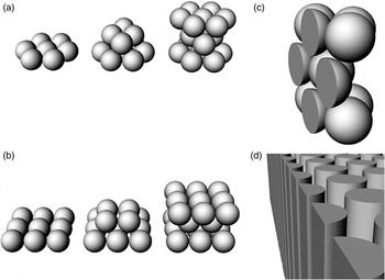
Although no recordings have yet been made of grids in a volumetric space, the experiment by Hayman et al. (Reference Hayman, Verriotis, Jovalekic, Fenton and Jeffery2011) of grids recorded on a vertical plane might have been expected to reveal evidence of periodicity in the vertical dimension, akin to what one would find by transecting a close-packed volume (Fig. 11c). However, that experiment found that the grid fields formed stripes on the vertical surface, implying instead that the true underlying pattern of grids in a volumetric space might be in the form of hexagonal close-packed columns (Fig. 11c). Whether this would also hold true for animals moving in an unconstrained way through the space remains to be seen. It is also possible that there is periodicity in the vertical dimension, but at a much greater scale than could be seen in a small laboratory setting.

5.1. Arguments for a bicoded cognitive map

The above possibilities concerning 3D maps notwithstanding, we suggest here that even ecologically three-dimensional animals may turn out to form planar, or quasi-planar, cognitive maps. Such animals often live in environments that are relatively more extended horizontally than vertically, making a planar map useful (particularly as almost all animals maintain a canonical body orientation with respect to gravity). Also, as discussed below, encoding three dimensions poses considerable technical challenges for a compass system. Indeed, there is little evidence for such integrated encoding in the species that have been studied so far. Head direction cells evidently operate in a plane rather than a volume, and grid cells are not periodic in the vertical dimension (or perhaps not in the dimension perpendicular to the animal's body plane).

In a bicoded map, there is a spatially metric representation of a reference plane – usually the horizontal plane – and a non-metric, or at least differently metricized, representation for the axis perpendicular to this plane. In the geographical example given earlier (Fig. 1c), the non-spatial indicator of distance was colour, which varies as a function of elevation but from which elevation cannot be extracted without a key. Loosely speaking, it is as if the non-metric variable conveys a coarse signal along the lines of “high” or “very high,” but does not contain explicit information about distance that could enter into a trigonometric calculation.

Obviously, the cognitive map does not use colour as its non-metric variable, but it could plausibly use an analogous signal, which we call here, for want of a better word, “contextual” – that is, information that pertains to a space but need not itself contain distance or direction information. A real-world example of a contextual elevation cue might be hydrostatic pressure, which Burt de Perera and colleagues put forward as a possible mechanism for fish to localize themselves in the vertical axis (Burt de Perera et al. Reference Burt de Perera, de Vos and Guilford2005). For terrestrial animals, it could be visual or kinaesthetic cues to ascent/descent, or aspects of the visual panorama; for flying animals, it could be depth cues from stereopsis or motion parallax, or perhaps olfactory gradients in the atmosphere.

Our hypothesis, then, is that the cognitive map is such a bicoded map – it is metric in a given plane (the plane of locomotion), and contextually modulated orthogonal to this. It is possible that contextual information concerning elevation could be processed by brain areas that are located outside the currently established navigation circuitry, although it is likely that these signals would interact at some point.

What evidence supports this bicoding view? Existing behavioural data from a number of studies, reviewed earlier, suggest a potential separation between horizontal and vertical dimensions. However, this does not prove that the encoding itself is different, merely that execution of navigational plans is different. Theoretically, this could be because the energetic costs of moving vertically are taken into account when planning, even if the planning is based on a fundamentally volumetric, three-dimensional map. The neural data, however, tell a more revealing story. The observation that head direction cells appear to use the plane of locomotion as a local reference (Stackman et al. Reference Stackman, Tullman and Taube2000) implies that the directional signal for the vertical plane (or rather, the plane normal to locomotion) must lie elsewhere, in an as yet undiscovered region. Furthermore, the finding that grid and place cells have different metric properties in the vertical dimension, at least for horizontally oriented body posture, implies that odometry does not take place equally in all three dimensions – the map is anisotropic (Hayman et al. Reference Hayman, Verriotis, Jovalekic, Fenton and Jeffery2011).

Note that it remains to be determined experimentally whether there is something special about the horizontal plane in the cognitive map, or whether it is simply that gravity primarily orients the locomotor plane and it is this plane that is metrically encoded. Recordings of grid cells on steeply sloping surfaces may answer this question.

A bicoded scheme seems suboptimal, but in fact a surface-travelling animal could do quite well with such a map, because it could use the metrically encoded locomotor plane to calculate the directions needed for travel, and the topography of the landscape would constrain the animal to be at the correct elevation for that position. Although a bicoded map could not be used for path integration in volumetric space, an animal could divide the navigational task into two parts: It could first calculate the horizontal trajectory and then ascend to the correct elevation (as indicated by the contextual gradient), or vice versa – or both simultaneously but in separate computational circuits. Indeed, the findings of Grobéty and Schenk (Reference Grobéty and Schenk1992a) seem to suggest that this is indeed what happens, at least in rats. However, in the case where “horizontal” is not true earth-horizontal, but lies on a slope, then it would be advantageous for the map to encode, in some form, information about that slope, as this would affect the energy costs of navigational routes involving that surface. Hence, there may be some mechanism for encoding the angle of a given planar fragment with respect to earth-horizontal.

A bicoded map has a planar metric reference, but as noted earlier, the real world is far from planar. How could a bicoded map be used on undulating topology? One possibility is that an undulating surface could be encoded as a manifold – not a single unified map, but a mosaic of contiguous map fragments. In such a scheme, each fragment would comprise a local reference frame defined by a reference plane (which would be horizontal on a horizontal surface, but need not be) and an axis orthogonal to this (which would correspond to the gravitationally defined vertical for an animal locomoting in its canonical orientation on a horizontal surface). Figure 12 shows an illustrative example of such a mosaicized representation. In the example, a rat, in a fairly short excursion, moves across the ground from a rock to a tree, up the trunk of the tree, and out onto a branch – each of these planes being orthogonal to the one before. To maintain orientation the animal must switch from a planar map referenced to the ground, to a new one referenced to the tree trunk, to a third referenced to the branch.

Figure 12.

Hypothetical structure of the cognitive map in a dimensionally complex environment. The map is assumed to be metric in the plane of locomotion, which is the ground for the space between the rock and the tree, the vertical trunk as the animal climbs, and the horizontal branch. The shading gradient represents the nonmetric encoding, which conveys coarse information about distance in the plane orthogonal to the locomotor plane, which is encoded differently from the precise metric of the locomotor plane.

If the planar fragments of the cognitive map need not be oriented horizontally, then how does the animal process the vertical axis, which remains a special, and important, reference due to the effects of gravity? To form an integrated map of large-scale space using mosaic fragments, there also should be some means of associating the local reference frames, both to one another (to enable navigation between fragments) and to earth-horizontal (to enable appropriate energy and other gravity-related calculations to be made). A plausible means of achieving this could be the vestibular system, which tracks changes in orientation via the semi-circular canals and could therefore provide some means of linking the map fragments together at, so to speak, their “edges.” With such a scheme it would be possible to use heuristic methods to compute, for example, approximate shortcuts between map fragments. For more sophisticated navigation, however, it would be preferable to weld fragments together into a larger, unitary frame that would allow for precise metric computations across the space. It may be that such a reference frame adaptation could occur with experience. In fact, the head direction cell studies of Stackman et al. (Reference Stackman, Tullman and Taube2000), in which reference frames could be local to the surface or more globally referenced to the surrounding room, support the possibility of such experience-dependent plasticity.

The possibility that the cognitive map is formed of a mosaic of locally planar fragments is consistent with the sudden reorientations experienced by humans and other animals as they transition from one region of the environment to the next (Wang & Spelke Reference Wang and Spelke2002). It is a commonplace experience of urban navigators when taking an unfamiliar route between two locally familiar places, for example, that a sudden, almost dizzying re-alignment of reference frames occurs across the interface between the two regions. This subjective experience may reflect the sudden reorientation of head direction cells that occurs when animals cross between local connected regions having different head direction cell orientations (Dudchenko & Zinyuk Reference Dudchenko and Zinyuk2005; Taube & Burton Reference Taube and Burton1995; Zugaro et al. Reference Zugaro, Arleo, Berthoz and Wiener2003). The reorientation episodes experienced by astronauts in conditions of microgravity may have a similar underlying cause (Oman Reference Oman, Mast and Jancke2007; See Fig. 12.)

What about subjects that habitually navigate in volumetric spaces, including animals such as fish, birds and bats, and also human divers, aviators and astronauts? Do they use a surface map too? In these environments, a plane-referenced map would seem much less useful. However, evidence from microgravity environment studies shows that even in a weightless environment, astronauts tend to find a reference plane to serve as a local “floor” (Oman Reference Oman, Mast and Jancke2007). This is usually the surface beneath their feet, but if they drift too far away from this “floor” and too far toward the “ceiling,” or switch visual attention, they frequently report visual reorientation illusions (VRIs), where surfaces abruptly and unexpectedly exchange identity (Oman et al. Reference Oman, Lichtenberg, Money and McCoy1986), testifying to the salience of the reference plane. Volume-travelling animals tend to maintain a constant body posture with respect to earth-horizontal and so they, too, may use a planar map for navigating, even though their movement in space is unconstrained.

5.2. Why would animals have a metrically planar map?

Why would animal cognitive maps be (quasi-)planar? On the face of it, this seems maladaptive, because a planar map, even a bicoded one, has inherently less information than a fully integrated volumetric one.

The first possibility is an ontogenetic one: that formation of the map during development is constrained by experience during infancy, and the animals that have been investigated to date have been, mainly for technical reasons, those species that are primarily surface-dwelling. An exception is fish, in which we also saw a processing separation between horizontal and vertical space (Holbrook & Burt de Perera Reference Holbrook and Burt de Perera2009), but this could have been a behavioural adaptation superimposed on an underlying volumetric map. It may be that if rats and mice were to be raised from birth in a volumetric space – for example, in microgravity, or at least in a lattice system in which they could move in all directions – then we would see true three-dimensional HD cells, and path integration behaviour that seamlessly encompassed all three dimensions.

Second, it may be that phylogenetic development of the map was so constrained, and therefore, surface-dwelling animals such as rats, mice, and humans would never develop a 3D map even if raised in conditions that would allow it. In other words, surface-dwellers have either lost or else never evolved the neurological capacity to fully represent three-dimensional space. However, if we were to study HD cells in animals that can move freely in all dimensions, then we may find three-dimensional HD cells in these species. Emerging studies in bats may soon answer this question, we hope. It should be noted, however, that rats and mice naturally inhabit dimensionally complex environments, and therefore might be expected to show integrated three-dimensional encoding if this ever did evolve in vertebrates.

The third and final possibility – and one for which we argue here – is that a fully 3D map has never evolved in any species, because of the difficulties inherent in stably encoding an allocentric three-dimensional space using egocentric sensory receptors. A volumetric map requires three coordinates for position and three for direction. Monitoring position and travel in such a space is complicated because the vestibular inputs to the head direction system originate in the semicircular canals, which are themselves planar (one aligned in each plane). In order to extract three-dimensional heading, the system would need to modulate the rotational signal from each canal with each of the other two, and do so dynamically and instantaneously. It is possible that the cost-benefit ratio of the required extra processing power is not sufficiently great, even for animals that have a three-dimensional ecological niche. As we saw in the four-dimension experiment of Aflalo and Graziano (Reference Aflalo and Graziano2008), it is possible to navigate quite well in a space using a lower-dimensional representation, together with some heuristics, and what applies in four dimensions may equally well apply in three.