


1. Introduction
As pointed out by Svante Janson in his seminal work [Reference Janson8], in many random combinatorial problems the interesting statistic is the sum of independent and identically distributed (i.i.d.) random variables conditioned on some exogenous integer-valued random variable. In general, the exogenous random variable is itself a sum of integer-valued random variables. Here, we are interested in the law of N −1(Y 1 + … + YN) conditioned on a specific value of X 1 + … + XN, that is, in the conditional distribution
 $${{\cal L}_N}\,: = {\cal L}({N^{ - 1}}({Y_1} + \cdots + {Y_N})\mid {X_1} + \cdots + {X_N} = m),$$
where m and N are integers and the (Xi, Yi) for 1 ≤ i ≤ N are i.i.d. copies of a vector (X, Y) of random variables with X integer valued.
Janson [Reference Janson8] proved a general central limit theorem (with convergence of all moments) for this kind of conditional distribution under some reasonable assumptions and gave several applications in classical combinatorial problems: occupancy in urns, hashing with linear probing, random forests, branching processes, etc. Following this work, one natural question arises: is it possible to obtain a general Berry–Esseen inequality for these models?
The first Berry–Esseen inequality for a conditional model is given by Malcolm P. Quine and John Robinson in [Reference Quine and Robinson17]. They study the particular case of the occupancy problem, i.e. the case when the random variable X is Poisson distributed and Y =1{X=0}. To the best of our knowledge, it is the only result in that direction for this kind of conditional distribution.
Our paper is organized as follows. In Section 2 we present the model and we state our main results (Theorems 1 and 2). In Section 3 we describe classical examples. The last section is dedicated to the proofs.
2. Conditional Berry–Esseen inequality
For all n ≥ 1, we consider a vector of random variables (Xn, Yn) such that Xn is integer valued and Yn real valued. Let Nn be a natural number such that Nn → ∞ as n goes to ∞. Let (Xn ,i, Y n,i)1≤i≤N n be an i.i.d. sample distributed as (Xn, Yn) and define
 $${S_{n,k}}: = \sum\limits_{i = 1}^k {\rm{ }} {X_{n,i}}\;\;\>{\rm{and}}\;\;\>{T_{n,k}}: = \sum\limits_{i = 1}^k {\rm{ }} {Y_{n,i}},$$
for  $k \in [\quad [1,N_n ]\quad ]$. To lighten notation, define Sn := Sn,N n and Tn := Tn,N n. Let mn ∈ ℤ be such that ℙ (Sn = mn) > 0. The purpose of the paper is to prove a Berry–Esseen inequality for the conditional distributions
 $${\cal L}({U_n}): = {\cal L}({T_n}|{S_n} = {m_n}).$$
Assumption 1. Suppose that there exist positive constants c 1, c̃ 2, c 2, c 3, c̃ 4, c 4, c 5, c 6, c 7, and η 0 such that
(A1)
 ${\gamma _n}: = 2\pi \sigma {X_n}N_n^{1/2}{\rm{\mathbb P}}({S_n} = {m_n}) \ge {C_1},$,
(A2) c̃ 2 ≤ σXn :=var (Xn)1/2 ≤ c 2,
(A3)
$\rho {X_n}: = {\rm{\mathbb E}}[|{X_n} - {\rm{\mathbb E}}[{X_n}]{|^3}] \le {c_3}\sigma _{{X_n}}^3,$,(A4) c̃ 4 ≤ σY n := var (Yn)1/2 ≤ c 4,
(A5)
$\rho {Y_n}: = {\rm{\mathbb E}}[|{Y_n} - {\rm{\mathbb E}}[{Y_n}]{|^3}] \le {c_5}\sigma _{{Y_n}}^3,$,(A6) the correlations
${r_n}: = cov\,({X_n},{Y_n})\sigma _{{X_n}}^{ - 1}\sigma _{{Y_n}}^{ - 1}$ satisfy |rn| ≤ c 6 <1,(A7) for
$Y'n\mathop :\nolimits_ = Yn - [Yn] - (Xn,Yn)X{n^{ - 2}}(Xn - [Xn])$, for all s ∈ [−ππ],and for all t ∈ [−η 0, η 0],
$|{\rm {\mathbb E}} [{e^{\rm{i}}}^{(s{X_n} + t{{Y'}_n})}]| \le 1 - {c_7}({\sigma _{Xn}}^2{s^2} + {\sigma _{{{Y'}_n}}}^2{t^2}).$






Obviously, Assumption 1 is very close to the set of assumptions of the central limit theorem established in [Reference Janson8, Theorem 2.3]. In particular, (A1) is a consequence of  $m_n = N_n {\rm{E}}[Xn] + O(XnN_n^{1/2} )$, (A3) and (A7) (see the proof of Theorem 2.3 of [Reference Janson8]). By [Reference Janson8, Lemma 4.1],
 ${\sigma _{{X_n}}}^2 \le 4{\rm{\mathbb E}}[|X - {\rm{\mathbb E}}[X]{|^3}]$, so c̃ 2 can be chosen as 1/(4). (A6) is not very restricting and holds in the examples provided in Section 3. Following [Reference Janson8], we introduce
 $Y'n$ in (A7) in order to work with a centred variable uncorrelated with Xn. If (X, Y′) is a vector of centred and uncorrelated random variables, then
 $$|{\rm {\mathbb E}}[{e^{\rm{i}}}^{(sX + tY')}]| = 1 - {1 \over 2}({\sigma _X}^2{s^2} + {\sigma _{Y'}}^2{t^2}) + o({s^2} + {t^2}),$$
so (A7) is reasonable if the vectors  $(Xn,Y'n)$ are identically distributed.
Proposition 1. Assume that
 $${m_n} = {N_n}{\rm{\mathbb E}}[Xn] + O(XnN_n^{1/2}),$$
that (Xn, Yn) converges in distribution to (X, Y) as n → ∞, and that, for every fixed r > 0,
 $$\mathop {\lim \,sup\,}\limits_{n \to \infty } {\rm{\mathbb E}}[|{X_n}{|^r}] < \infty \quad {\rm{and}}\quad \mathop {\lim \,sup}\limits_{n \to \infty } {\rm{\mathbb E}}[|Yn{|^r}] < \infty .$$
Suppose further that the distribution of X has span 1 and that Y is not almost surely equal to an affine function c + dX of X. Then, Assumption 1 is satisfied.
The proof is omitted since the proposition relies on Corollary 2.1 and Theorem 2.3 of [Reference Janson8].
Theorem 1. Under Assumption 1,  $\tau _n^2\mathop :\nolimits_ = Y{n^2}(1 - r_n^2) > 0$ and we have
 $$\mathop {\sup }\limits_{x \in {\rm{\mathbb R}}} |{\rm{\mathbb P}}({{{U_n} - {N_n}{\rm{\mathbb E}}[Yn] - {r_n}YnX{n^{ - 1}}({m_n} - {N_n}{\rm{E}}[Xn])} \over {N_n^{1/2}{\tau _n}}}x) - \Phi (x)|{C \over {N_n^{1/2}}},$$
where Φ denotes the standard normal cumulative distribution function and C is a positive constant that depends only on c̃ 2, c 2, c 3, c̃ 4, c 4, c 5, c 6, c 7, η 0, and c 1.
Remark that the standardization of the variables Un involved in (1) is not the natural one. The following theorem fixes this default of standardization.
Proposition 2. Under (A1), (A3), (A4), (A5), and (A7), there exist two positive constants d 1 and d 2 depending only on c 3, c 4, c 5, c 7, and c 1 such that, for Nn ≥ 3,
 $$|{\rm{\mathbb E}}[{U_n}] - {N_n}{\rm{\mathbb E}}[Yn] - {r_n}YnX{n^{ - 1}}({m_n} - {N_n}{\rm{\mathbb E}}[Xn])| \le {\rm {d_1}}$$
and
 $$|{\rm {var}}({U_n}) - {N_n}\tau _n^2| \le {\rm {d_2}} N_n^{1/2}.$$
Theorem 2. Under Assumption 1, we have
 $$\mathop {\sup }\limits_{x \in {\rm{\mathbb R}}} |{\rm{\mathbb P}}({{{U_n} - {\rm{E}}[{U_n}]} \over {{{({U_n})}^{1/2}}}}x) - \Phi (x)|{{\widetilde C} \over {N_n^{1/2}}},$$
where C̃ is a constant that depends only on c̃ 2, c 2, c 3, c̃ 4, c 4, c 5, c 6, c 7, η 0, and c 1.
Furthermore, as in [Reference Janson8], the results of Theorems 1 and 2 simplify considerably in the special case when the vector (Xn, Yn) does not depend on n, that is, when we consider an i.i.d. sequence instead of a triangular array. This is a consequence of Proposition 1.
3. Classical examples
In this section we describe the examples mentioned in [Reference Holst6] and [Reference Janson8]. Each example satisfies the assumptions of Proposition 1, as shown in [Reference Janson8], leading to a Berry–Esseen inequality.
3.1. Occupancy problem
In the classical occupancy problem, m balls are thrown uniformly at random into N urns. The resulting numbers of balls (Z 1, …, ZN) have a multinomial distribution. It is well known that (Z 1, …, ZN) is also distributed as (X 1, …, XN) conditioned on 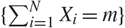 $\{ \sum\nolimits_{i = 1}^N X_i = m\}$, where the random variables Xi are i.i.d., with
 $X_i \sim {\cal P}(\lambda )$ for any arbitrary λ > 0. The classical occupancy problem studies the number of empty urns
 $U = \sum\nolimits_{i = 1}^N 1_{\{ Z_i = 0\} }$, which is distributed as
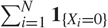 $\sum\nolimits_{i = 1}^N 1_{\{ X_i = 0\} }$ conditioned on
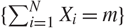 $\{ \sum\nolimits_{i = 1}^N X_i = m\}$. Now, if m = mn → ∞ and N = Nn → ∞ with mn/Nn → λ ∈ (0, ∞), we can take
 $Xn \sim {\cal P}(\lambda _n )$ with λn := mn/Nn, Yn = 1{X n=0}, and apply Proposition 1 to obtain a Berry–Esseen inequality for
 $U_n = \sum\nolimits_{i = 1}^{N_n } 1_{\{ Z_i = 0\} }$.
Remark 1. In [Reference Quine and Robinson17], the authors proved a Berry–Esseen inequality for the occupancy problem in a more general setting: the probability of landing in each urn may be different. The tools they developed will be used below to prove our results.
Remark 2. Here, we need a result for triangular arrays, and not only for i.i.d. sequences. Indeed, if we took Xn = X with  $X \sim \mathcal{P}(\lambda)$, we would only have
 $${m_n} = {N_n}(\lambda + o(1)) = {N_n}{\rm{\mathbb E}}[Xn] + o({N_n}).$$
But Proposition 1 requires
 $${m_n} = {N_n}{\rm{\mathbb E}}[X] + O(N_n^{1/2}),$$
which is stronger. This remark goes for the following examples too.
3.2. Bose–Einstein statistics
This example is borrowed from [Reference Holst6] (see also [Reference Feller3]). Consider N urns and put m indistinguishable balls in the urns in such a way that each distinguishable outcome has the same probability  $1/\left( {\matrix{
{m + N - 1} \cr
m \cr
} } \right)$. Let Zk be the number of balls in the kth urn. It is well known that (Z 1, …, ZN) is distributed as (X 1, …, XN) conditioned on
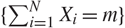 $\{ \sum\nolimits_{i = 1}^N X_i = m\}$, where the random variables Xi are i.i.d., with
 $X_i \sim {\cal G}(p)$ for any arbitrary p ∈ (0, 1). If m = n, N = Nn → ∞ with Nn/n → p, take
 $Xn \sim {\cal G}(p_n )$ with pn = Nn/n to obtain a Berry–Esseen inequality for any sequence of variables of the type
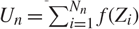 $U_n = \sum\nolimits_{i = 1}^{N_n } f(Z_i )$.
3.3. Branching processes
Consider a Galton–Watson process, beginning with one individual, where the number of children of an individual is given by a random variable X having finite moments. Assume further that  ${\rm{E}}[X] = 1$. We number the individuals as they appear. Let Xi be the number of children of the ith individual and
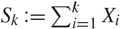 $S_k \mathop :\nolimits_ = \sum\nolimits_{i = 1}^k X_i$. It is well known (see [Reference Janson8, Example 3.4] and the references therein) that the total progeny SN + 1 is N ≥ 1 if and only if, for all k ∈ {0, …, N −1},
 \begin{equation}
S_k \geq k \quad\text{and}\quad S_N = N-1 .
\end{equation}
This type of conditioning is different from the one studied in the present paper, but, by [Reference Wendel18, Corollary 2] and [Reference Janson8, Example 3.4], if we ignore the cyclical order of X 1, …, XN, it is proved that X 1, …, XN, have the same distribution conditioned on (5) as conditioned on {SN = N − 1}. Applying Proposition 1 with N = n and m = n − 1, we obtain a Berry–Esseen inequality for any sequence of variables Un distributed as  $T_n = \sum\nolimits_{i = 1}^n f(X_i )$ conditioned on {SN = n − 1}. For instance, if f (x) = 1{x=3}, Un is the number of individuals with three children given that the total progeny is n.
3.4. Random forests
Consider a uniformly distributed random labelled rooted forest with m vertices and N roots with N < m. Without loss of generality, we may assume that the vertices are 1, …, m and, by symmetry, that the roots are the first N vertices. Following [Reference Janson8], this model can be realized as follows. The sizes of the N trees in the forest are distributed as (X 1, …, XN) conditioned on 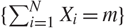 $\{ \sum\nolimits_{i = 1}^N X_i = m\}$, where the random variables Xi are i.i.d. and Borel distributed for any arbitrary parameter μ ∈ (0, 1), i.e.
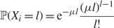 $${\rm{\mathbb P}}({X_i} = l{) = ^{ - \mu l}}{{{{(\mu l)}^{l - 1}}} \over {l{\kern 1pt} !{\kern 1pt} }}$$
(see, e.g. [Reference Flajolet, Poblete and Viola5] or [Reference Janson7] for more details). Then the ith tree is drawn uniformly among the trees of size Xi. Proposition 1 provides a Berry–Esseen inequality for any sequence of variables of the type 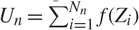 $U_n = \sum\nolimits_{i = 1}^{N_n } f(Z_i )$ where Nn → ∞and Z 1, …, ZN n are the sizes of the trees in the forest. For instance, if f (x) = 1{x= K}, Un is the number of trees of size K in the forest (see, e.g. [Reference Kolchin12], [Reference Pavlov15], and [Reference Pavlov16]).
3.5. Hashing with linear probing
Hashing with linear probing is a classical model in theoretical computer science that appeared in the 1960s. It was first studied from a mathematical point of view in [Reference Knuth10]. For more details on the model, we refer the reader to [Reference Chassaing and Flajolet1], [Reference Chassaing and Louchard2], [Reference Flajolet, Poblete and Viola5], [Reference Janson7], [Reference Janson9], and [Reference Marckert14]. The model describes the following experiment. One throws n balls sequentially into m urns at random with m > n; the urns are arranged in a circle and numbered clockwise. A ball that lands in an occupied urn is moved to the next empty urn, always moving clockwise. The length of the move is called the displacement of the ball and we are interested in the sum of all displacements which is a random variable denoted by dm ,n. After throwing all balls, there are N := m − n empty urns. These divide the occupied urns into blocks of consecutive urns. We consider that the empty urn following a block belongs to this block. Following [Reference Flajolet, Poblete and Viola5] and [Reference Knuth11], Janson [Reference Janson7] proved that the lengths of the blocks and the sums of displacements inside each block are distributed as (X 1, Y 1), …, (XN, YN) conditioned on 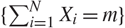 $\{ \sum\nolimits_{i = 1}^N X_i = m\}$, where the random vectors (Xi, Yi) are i.i.d. copies of a vector (X, Y) of random variables, X being Borel distributed with any arbitrary parameter μ ∈ (0, 1) and Y given {X = l} being distributed as dl ,l−1. In particular, dm ,n is distributed as
 $\sum\nolimits_{i = 1}^N Y_i$ conditioned on
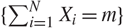 $\{ \sum\nolimits_{i = 1}^N X_i = m\}$. If m= mn → ∞ and N = Nn = mn − n → ∞ with n/mn→μ ∈ (0, 1), we take Xn following Borel distribution with parameter μn := n/mn to get a Berry–Esseen inequality for dmn ,n, by Proposition 1.
4. Proofs
Recall that Un is distributed as Tn conditioned on {Sn = mn}. Following the procedure of [Reference Janson8], we consider the projection
 $$Y'n = Yn - {\rm{\mathbb E}}[Yn] - (Xn,Yn)X{n^{ - 2}}(Xn - {\rm{\mathbb E}}[Xn]).$$
Then  ${\rm{E}}[Y'n] = 0$ and
 ${\rm{cov }}(Xn,Y'n) = {\rm{E}}[XnY'n] = 0$. Besides, (A7) and (A6) are verified by
 $Y'n$. By (A6),
 $${\sigma _{{{Y'}_n}}}^2 = {\sigma _{{Y_n}}}^2(1 - r_n^2) \in [{\tilde c_4}^2(1 - {c_6}^2),{c_4}^2],$$
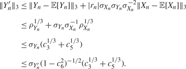
so (A4) is satisfied by  $Y'n$. Finally, by the Minkowski inequality, (A3), (A5), and the fact that |rn| ≤ 1,
 $$\matrix{
{\parallel {{Y'}_n}{\parallel _3}} \hfill & \le \hfill & {\parallel {Y_n} - {\rm{\mathbb E}}[Yn]{\parallel _3} + |{r_n}|{\sigma _{{X_n}}}{\sigma _{{Y_n}}}{\sigma _{{X_n}}}^{ - 2}\parallel {X_n} - {\rm{\mathbb E}}[{X_n}]{\parallel _3}} \hfill \cr
{} \hfill & \le \hfill & {{\rho _{{Y_n}}}^{1/3} + {\sigma _{{Y_n}}}{\sigma _{{X_n}}}^{ - 1}{\rho _{{X_n}}}^{1/3}} \hfill \cr
{} \hfill & \le \hfill & {{\sigma _{{Y_n}}}({c_3}^{1/3} + {c_5}^{1/3})} \hfill \cr
{} \hfill & \le \hfill & {\sigma {{Y'}_n}{{(1 - c_6^2)}^{ - 1/2}}({c_3}^{1/3} + {c_5}^{1/3}).} \hfill \cr
} $$
Hence,  $Y'n$ satisfies (A5). Consequently, all conditions hold for the vector
 $(Xn,Y'n)$ too. Finally,
 $${T'_n}\mathop :\limits_ = \sum\limits_{i = 1}^{{N_n}} {Y'_{n,i}} = {T_n} - {N_n}{\rm{\mathbb E}}[{Y_n}] - {\mathop{\rm cov}} ({X_n},{Y_n}){X_{{X_n}}}^{ - 2}({S_n} - {N_n}{\rm{\mathbb E}}[{X_n}]).$$
So, conditioned on {Sn = mn}, we have
 $${T'_n} = {T_n} - {N_n}{\rm{\mathbb E}}[{Y_n}] - {r_n}{\sigma _{{Y_n}}}{\sigma _{{X_n}}}^{ - 1}({m_n} - {N_n}{\rm{\mathbb E}}[{X_n}]).$$
Hence, the conclusions in Theorems 1 and 2 for (Xn, Yn) and  $(Xn,Y'n)$ are the same. Thus, it suffices to prove the theorems for
 $(Xn,Y'n)$. In other words, we will henceforth assume that
 ${\rm{E}}[Yn] = {\rm{E}}[XnYn] = 0$, rn = 0 and
 $\tau _n^2 = {\rm{ }}\sigma Yn^2$. Moreover, the constants
 $c_4^{'}$,
 $\tilde c_4^{'}$,
 $c_5^{'}$,
 $c_6^{'}$, and
 $c_7^{'}$ for (X, Y′) are linked to that of (X, Y) by the following relations:
 $c_4^{'} = {c_{4}}$,
 $\tilde c_4^{'} = {\tilde c_4}{(1 - c_6^2)^{1/2}}$,
 $\tilde c_5^{'} = {(1 - c_6^2)^{1/3}}{(c_3^{1/3} + c_5^{1/3})^3}$,
 $c_6^{'} = 0$, and
 $c_7^{'} = {c_7}$. In the proofs we omit the primes.
The proofs of Theorems 1 and 2 intensively rely on the use of Fourier transforms through the functions φn and ψn defined by
 $${\varphi _n}(s,t)\mathop :\limits_ = {\rm{\mathbb E}}[\exp \{ {\rm{i}}s({X_n} - {\rm{\mathbb E}}[{X_n}]) + {\rm{i}}t{Y_n}\} ],\quad \quad {\psi _n}(t)\mathop :\limits_ = 2\pi P({S_n} = {m_n}){\rm{\mathbb E}}[\exp \{ {\rm{i}}t{U_n}\} ].$$
The controls of these functions (respectively the controls of their derivatives) needed in the proofs are postponed to Lemmas 1 and 2 in Section 4.4 (respectively Lemma 3). In particular, (15)–(18) will be used several times below.
4.1. Proof of Theorem 1
We follow the classical proof of Berry–Esseen theorem (see, e.g. [Reference Feller4]) combined with the procedure in [Reference Quine and Robinson17]. As shown in [Reference Loève13, p. 285] or [Reference Feller4], the left-hand side of (1) is dominated by
 \[\frac{2}{\pi }\int_{0}^{\eta \sigma {{Y}_{n}}N_{n}^{1/2}}{}|\frac{{{\psi }_{n}}(u\sigma _{{{Y}_{n}}}^{-1}N_{n}^{-1/2})}{2\pi {\rm {\mathbb P}}({{S}_{n}}={{m}_{n}})}{{-}^{-{{u}^{2}}/2}}|\frac{\text{d}u}{u}+\frac{24\sigma _{{{Y}_{n}}}^{-1}N_{n}^{-1/2}}{\eta \pi \sqrt{2\pi }},\]
where η > 0 is arbitrary. We choose to define
 $$\eta : = \min ({2 \over 9}{({c_4}{c_5})^{ - 1}},\,{\eta _0}) > 0.$$
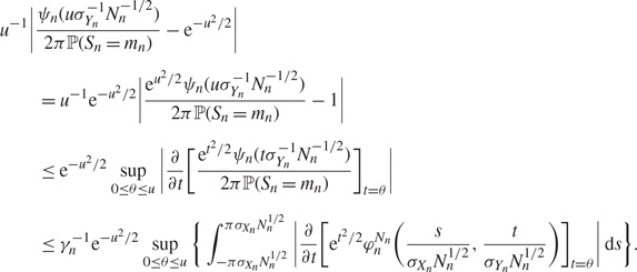
From (15) of Lemma 1 and using Taylor’s expansion,
 $$\eqalign{
& {u^{ - 1}}|{{{\psi _n}(u\sigma _{{Y_n}}^{ - 1}N_n^{ - 1/2})} \over {2\pi {\rm{\mathbb P}}({S_n} = {m_n})}} - {{\rm{e}}^{ - {u^2}/2}}| \cr
& \matrix{
{ = {u^{ - 1}}^{ - {u^2}/2}|{{{{\rm{e}}^{{u^2}/2}}{\psi _n}(u\sigma _n^{ - 1/2})} \over {2\pi {\rm{P}}({S_n} = {m_n})}} - 1|} \hfill \cr
{{ \le ^{ - {u^2}/2}}\mathop {\sup }\limits_{0 \le \theta \le u} |{\partial \over {\partial t}}{{\left[ {{{{{\rm{e}}^{{t^2}/2}}{\psi _n}(t\sigma _{{Y_n}}^{ - 1}N_n^{ - 1/2})} \over {2\pi ({S_n} = {m_n})}}} \right]}_{t = \theta }}|} \hfill \cr
{ \le {\gamma _n}^{ - 1}{{\rm{e}}^{ - {u^2}/2}}\mathop {\sup }\limits_{0 \le \theta \le u} \left\{ {\int_{ - \pi {\sigma _{{X_n}}}N_n^{1/2}}^{\pi {\sigma _{{X_n}}}N_n^{1/2}} |{\partial \over {\partial t}}{{\left[ {{e^{{t^2}/2}}\varphi _n^{{N_n}}\left( {{s \over {{\sigma _{{X_n}}}N_n^{1/2}}},{t \over {{\sigma _{{Y_n}}}N_n^{1/2}}}} \right)} \right]}_{t = \theta }}|{\rm{d}}s} \right\}.} \hfill \cr
} \cr} $$
By (A1), γn ≥ c 1.Now we split the integration domain of s into
 $${A_1}\mathop :\limits_ = \{ s:|s| < \varepsilon \} \quad {\rm{and}}\quad {A_2}\mathop :\limits_ = \{ s:\varepsilon |s| \le \pi \} ,$$
where
 $$\varepsilon : = \min ({\textstyle{2 \over 9}}{({c_2}{c_3})^{ - 1}},\pi ),$$
and decompose
 $${u^{ - 1}}|{{{\psi _n}(u\sigma _{{Y_n}}^{ - 2/2})} \over {2\pi {\rm{\mathbb P}}({S_n} = {m_n})}} - {{\rm{e}}^{ - {u^2}/2}}| \le \mathop {\sup }\limits_{0 \le \theta \le u} [{I_1}(n,u,\theta ) + {I_2}(n,u,\theta )],$$
where
 $${I_1}(n,u,\theta ) = {\gamma _n}^{ - 1}\int_{{A_1}} {{\rm{e}}^{ - ({u^2} + {s^2})/2}}|{\partial \over {\partial t}}{\left[ {{{\rm{e}}^{({t^2} + {s^2}}}\varphi _n^{{N_n}}\left( {{s \over {{\sigma _{{X_n}}}N_n^{1/2}}},{t \over {{\sigma _{{Y_n}}}N_n^{1/2}}}} \right)} \right]_{t = \theta }}|{\rm{d}}s,$$
 $${I_2}(n,u,\theta ) = {\gamma _n}^{ - 1}{{\rm{e}}^{ - {u^2}/2}}\int_{{A_2}} |{\partial \over {\partial t}}{\left[ {{{\rm{e}}^{{t^2}/2}}\varphi _n^{{N_n}}\left( {{s \over {{\sigma _{{X_n}}}N_n^{1/2}}},{t \over {{\sigma _{{Y_n}}}N_n^{1/2}}}} \right)} \right]_{t = \theta }}|{\rm{d}}s.$$
Lemmas 5 and 6 state that there exists positive constants C 1 and C 2, depending only on c̃ 2, c 2, c 3, c 5, c 7, and c 7 such that, for  ${N_n} \ge \max {(12^3}^2{,12^3}^2,2),$,
 $$\int_0^{\eta {\sigma _{{Y_n}}}N_n^{1/2}} \mathop {\sup }\limits_{0 \le \theta \le u} {I_1}(n,u,\theta )u \le {{{C_1}} \over {N_n^{1/2}}},$$
and
 $$\int_0^{\eta {\sigma _{{Y_n}}}N_n^{1/2}} \mathop {\sup }\limits_{0 \le \theta \le u} {I_2}(n,u,\theta )u \le {{{C_2}} \over {N_n^{1/2}}},$$
So,
 $$\mathop {\sup }\limits_{x \in {\rm{\mathbb R}}} |{\rm{\mathbb P}}({{{U_n}} \over {N_n^{1/2}{\sigma _Y}_{_n}}} \le x) - \Phi (x)| \le {C \over {N_n^{1/2}}}$$
with
 $$C: = \max \left( {{C_1} + {C_2} + {{24} \over {\widetilde {c4}\pi \sqrt {2\pi } {\kern 1pt} }}{{\left( {\min \left( {{2 \over 9},{c_4}{s_5}{\eta _0}} \right)} \right)}^{ - 1}}{{,12}^{3/2}}{c_3}{{,12}^{3/2}},\sqrt 2 } \right).$$
4.2. Proof of Proposition 2
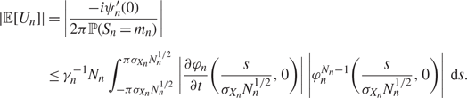
Proof of (2). We adapt the proof given in [Reference Janson8]. Using the definition of Ψn given in (6), and differentiating under the integral sign of (15) of Lemma 1, we naturally have
 $$\matrix{
{|{\rm{\mathbb E}}[{U_n}]| = \left| {{{ - i\psi _n^{'}(0)} \over {2\pi {\rm{\mathbb P}}({S_n} = {m_n})}}} \right|} \hfill \cr
{ \le {\gamma _n}^{ - 1}{N_n}\int_{ - \pi \sigma {X_n}N_n^{1/2}}^{\pi {\sigma _{{X_n}}}N_n^{1/2}} \left| {{{\partial {\varphi _n}} \over {\partial t}}\left( {{s \over {{\sigma _{{X_n}}}N_n^{1/2}}},0} \right)} \right|\left| {\varphi _n^{{N_n} - 1}\left( {{s \over {{\sigma _{{X_n}}}N_n^{1/2}}},0} \right)} \right|{\rm{d}}s.} \hfill \cr
} $$
Using (18) of Lemma 3 with t = 0, (A2), (A3), and (A5), we deduce that
 $$\left| {{{\partial {\varphi _n}} \over {\partial t}}\left( {{s \over {{\sigma _{{X_n}}}N_n^{1/2}}},0} \right)} \right| \le {{{s^2}} \over 2}{{\rho _{{Y_n}}^{1/3}{\rho _{{X_n}}}^{2/3}} \over {{\sigma _{{X_n}}}^2{N_n}}} \le {{{c_3}^{2/3}{c_5}^{1/3}} \over {2{N_n}}}{s^2}.$$
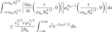
Then, using (16) of Lemma 2 (with l = 1 and t = 0) and for Nn ≥ 3,
 $$\matrix{
{\int_{ - \pi {\sigma _{{X_n}}}N_n^{1/2}}^{\pi {\sigma _{{X_n}}}N_n^{1/2}} \left| {{{\partial {\varphi _n}} \over {\partial t}}\left( {{s \over {{\sigma _{{X_n}}}N_n^{1/2}}},0} \right)||\varphi _n^{{N_n} - 1}({s \over {{\sigma _{{X_n}}}N_n^{1/2}}},0)} \right|{\rm{d}}s} \hfill \cr
{\quad \quad \le {{{c_3}^{2/3}{c_5}^{1/3}} \over {2{N_n}}}\int_{ - \infty }^{ + \infty } {s^2}{{\rm{e}}^{ - 2{s^2}/3}}{\rm{d}}s.} \hfill \cr
} $$
So, (2) holds with
 $${d_1}: = {2^{ - 1}}{c_3}^{2/3}{c_5}^{1/3}{c_1}^{ - 1}\int_{ - \infty }^{ + \infty } {s^2}{{\rm{e}}^{ - 2{c_7}{s^2}/3}}{\rm{d}}s.$$
Proof of (3) Since  $\tau _n^2 = Yn^2$ and
 ${\rm{E}}[U_n ]$ is bounded, it suffices to show that the quantity
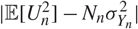 $|{\rm{E}}[U_n^2 ] - N_n Yn^2 |$ is bounded by some
 $N_n^{1/2}$ to prove (3). Proceeding as before,
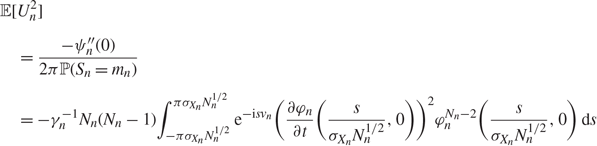 $$\eqalign{
& {\rm{E}}[U_n^2] \cr
& \matrix{
{\quad = {{ - {{\psi {''}}_n}(0)} \over {2\pi {\rm{P}}({S_n} = {m_n})}}} \hfill \cr
{\quad = - {\gamma _n}^{ - 1}{N_n}({N_n} - 1)\int_{ - \pi {\sigma _{{X_n}}}{N^{1/2}}_n}^{\pi {\sigma _{{X_n}}}{N^{1/2}}_n} {e^{ - is{v_n}}}{{\left( {{{\partial {\varphi _n}} \over {\partial t}}\left( {{s \over {{\sigma _{{X_n}}}N_n^{1/2}}},0} \right)} \right)}^2}\varphi _n^{{N_n} - 2}\left( {{s \over {{\sigma _{{X_n}}}N_n^{1/2}}},0} \right){\rm{d}}s} \hfill \cr
} \cr} $$
 $$ - {\gamma _n}^{ - 1}{N_n}\int_{ - \pi {\sigma _{{X_n}}}{N^{1/2}}_n}^{\pi {\sigma _{{X_n}}}{N^{1/2}}_n} {e^{ - is{v_n}}}\left( {{s \over {{\sigma _{{X_n}}}N_n^{1/2}}},0} \right)\varphi _n^{{N_n} - 1}\left( {{s \over {{\sigma _{{X_n}}}N_n^{1/2}}},0} \right){\rm{d}}s,$$
where
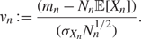 $${v_n}: = {{({m_n} - {N_n}{\rm{\mathbb E}}[Xn])} \over {({\sigma _{{X_n}}}N_n^{1/2})}}.$$
First, by (18) of Lemma 3 with t = 0 and by (16) of Lemma 2 (with l = 2 and t = 0), we have, for Nn ≥ 3,
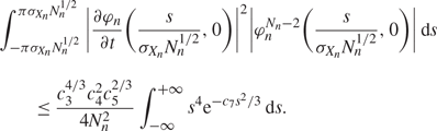 $$\matrix{
{\int_{ - \pi {\sigma _{{X_n}}}N_n^{1/2}}^{\pi {\sigma _{{X_n}}}N_n^{1/2}} \left| {{{\partial {\varphi _n}} \over {\partial t}}{{\left( {{s \over {{\sigma _{{X_n}}}N_n^{1/2}}},0} \right)}^2}} \right|\left| {\varphi _n^{{N_n} - 2}\left( {{s \over {{\sigma _{{X_n}}}N_n^{1/2}}},0} \right)} \right|{\rm{d}}s} \hfill \cr
{\quad \quad \le {{{c_3}^{4/3}c_4^2{c_5}^{2/3}} \over {4N_n^2}}\int_{ - \infty }^{ + \infty } {s^4}{{\rm{e}}^{ - {c_7}{s^2}/3}}{\rm{d}}s.} \hfill \cr
} $$
Finally, by (A1), the term (13) is bounded by
 $${d{''}_2}: = {{{c_3}^{4/3}{c_4}^2{c_5}^{2/3}} \over {4{c_1}}}\int_{ - \infty }^{ + \infty } {s^4}{{\rm{e}}^{ - {c_7}{s^2}/3}}{\rm{d}}s.$$
Second, we study the term (14). We want to show that
 $${\Delta _n}: = {\gamma _n}^{ - 1}\int_{ - \pi {\sigma _{Xn}}N_n^{1/2}}^{\pi {\sigma _{Xn}}N_n^{1/2}} \,{e^{ - {\rm{i}}s{v_n}}}{{{\partial ^2}{\varphi _n}} \over {\partial {t^2}}}\left( {{s \over {{\sigma _{Xn}}N_n^{1/2}}},0} \right)\varphi _n^{{N_n} - 1}\left( {{s \over {{\sigma _{Xn}}N_n^{1/2}}},0} \right){\rm{d}}s + {\sigma _{{Y_n}}}^2$$
is bounded by some  $d_2^{'''}/N_n^{1/2}$. By (15) with t = 0,
 $$\int_{ - \pi {\sigma _{{X_n}}}N_n^{1/2}}^{\pi {\sigma _{{X_n}}}N_n^{1/2}} \,{{\rm{e}}^{ - {\rm{i}}s{v_n}}}\varphi _n^{{N_n}}\left( {{s \over {{\sigma _X}_nN_n^{1/2}}},0} \right){\rm{d}}s = 2\pi {\rm{P}}({S_n} = {m_n}){\sigma _X}_nN_n^{1/2} = {\gamma _n},$$
so
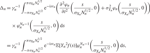 $$\matrix{
{{\Delta _n}{ = ^{ - 1}}{{\int_{ - \pi }^\pi }^{ - s{v_n}}}({{{\partial ^2}{\varphi _n}} \over {\partial {t^2}}}(\underline s,0) + Y{n^2}{\varphi _n}(\underline s,0))} \hfill \cr
{\quad \times \varphi _n^{{N_n} - 1}(\underline s,0)s} \hfill \cr
{{ = ^{ - 1}}{{\int_{ - \pi }^\pi }^{ - s{v_n}}}{\rm{E}}[Y{n^2}f(s)]\varphi _n^{{N_n} - 1}(\underline s,0)s,} \hfill \cr
} $$
where
 $$f(s) = - ({e^{{\rm{i}}s{\sigma ^{ - 1}}_{{X_n}}N_n^{ - 1/2}(Xn - {\rm{\mathbb E}}[Xn])}} - {\rm{\mathbb E}}{[^{{e^{{\rm{i}}s{\sigma ^{ - 1}}_{{X_n}}N_n^{ - 1/2}(Xn - {\rm{\mathbb E}}[Xn])}}}}]).$$
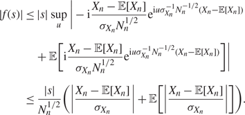
Applying Taylor’s theorem yields
 $$\matrix{
{|f(s)| \le |s|\mathop {\sup }\limits_u | - {\rm{i}}{{{X_n} - {\rm{\mathbb E[}}{{\rm{X}}_n}{\rm{]}}} \over {{\sigma _{{X_n}}}N_n^{1/2}}}{\rm{ei}}u\sigma _{{X_n}}^{ - 1}N_n^{ - 1/2}({X_n} - {\rm{\mathbb E}}[{X_n}])} \cr
{ + {\rm{\mathbb E}}\left[ {{\rm{i}}{{{X_n} - {\rm{\mathbb E[}}{X_n}{\rm{]}}} \over {\sigma {X_n}N_n^{1/2}}}{{\rm{e}}^{{\rm{i}}u\sigma }}X_n^{ - 1}N_n^{ - 1/2}({X_n} - E[{X_n}])} \right]|} \cr
{ \le {{|s|} \over {N_n^{1/2}}}\left( {\left| {{{Xn - {\rm{\mathbb E}}[{X_n}]} \over {\sigma {X_n}}}} \right| + {\rm{\mathbb E}}\left[ {\left| {{{{X_n} - {\rm{\mathbb E}}[{X_n}]} \over {\sigma {X_n}}}} \right|} \right]} \right).} \cr
} $$
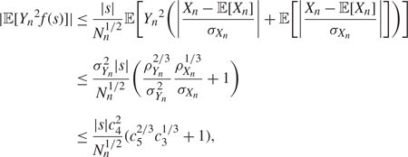
Thus, using Hölder’s inequality,
 $$\matrix{
{|{\rm{\mathbb E}}[{Y_n}^2f(s)]| \le {{|s|} \over {N_n^{1/2}}}{\rm{\mathbb E}}Y{n^2}\left[ {\left( {|{{Xn - {\rm{E}}[{X_n}]} \over {{X_n}}}| + {\rm{\mathbb E}}\left[ {|{{{X_n} - {\rm{\mathbb E}}[{X_n}]} \over {{X_n}}}|} \right]} \right)} \right]} \cr
{ \le {{{\sigma _{{Y_n}}}^2|s|} \over {N_n^{1/2}}}\left( {{{{\rho _{{Y_n}}}^{2/3}} \over {{\sigma _{{Y_n}}}^2}}{{{\rho _{{X_n}}}^{1/3}} \over {{\sigma _{{X_n}}}}} + 1} \right)} \cr
{ \le {{|s{|^2}} \over {N_n^{1/2}}}({c_5}^{2/3}{c_3}^{1/3} + 1),} \cr
} $$
where the last inequality is obtained using (A2)–(A5). Now, by (A1) and the upper bound in (16) (with l = 1 and t = 0), we get, for Nn ≥ 3,
 $$|{\Delta _n}| \le {{{c_4}^2} \over {{c_1}N_n^{1/2}}}({c_5}^{2/3}{c_3}^{1/3} + 1)\int_{ - \infty }^{ + \infty } |s|{{\rm{e}}^{ - {s^2}{c_7}({N_n} - 1)/{N_n}}}{\rm{d}}s \le {{d_2^{'''}} \over {N_n^{1/2}}},$$
with
 $$d_2^{'''}: = {c_4}^2{c_1}^{ - 1}({c_5}^{2/3}{c_3}^{1/3} + 1)\int_{ - \infty }^{ + \infty } |s|{{\rm{e}}^{ - 2{s^2}c7/3}}{\rm{d}}s.$$
Finally,
 $$|{\mathop{\rm var}} ({U_n}) - {N_n}{\sigma _{{Y_n}}}^2| \le ({d_1}^2 + d_2^{''} + d_2^{'''})N_n^{1/2} = :{d_2}{\kern 1pt} N_n^{1/2}.$$
The proof of (3) is complete.
4.3. Proof of Theorem 2
Write
 $$\matrix{
{|{\rm{\mathbb P}}\left( {{{{U_n} - {\rm{\mathbb E}}[{U_n}]} \over {{\mathop{\rm var}} {{({U_n})}^{1/2}}}} \le x} \right) - \Phi (x)|} \hfill \cr
{\quad \quad \le |{\rm{\mathbb P}}({{{U_n}} \over {N_n^{1/2}{Y_n}}}{a_n}x + {b_n}) - \Phi ({a_n}x + {b_n})| + |\Phi ({a_n}x + {b_n}) - \Phi (x)|,} \hfill \cr
} $$
where
 $${a_n}: = {{{\mathop{\rm var}} {{({U_n})}^{1/2}}} \over {N_n^{1/2}\sigma {Y_n}}}\quad {\rm{and}}\quad {b_n}: = {{{\rm{\mathbb E}}[{U_n}]} \over {N_n^{1/2}\sigma {Y_n}}}.$$
The previous estimates of  ${\rm{\mathbb E}}[U_n ]$ and (Un) yield
 $$|{a_n} - 1| \le |a_n^2 - 1| \le {d_2}{\tilde c_4}^{ - 2}N_n^{ - 1/2}\quad {\rm{and}}\quad |{b_n}| \le {d_1}{\tilde c_4}^{ - 1}N_n^{ - 1/2}.$$
Then, for 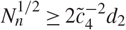 $N_n^{1/2} \ge 2^{ - 2}$,
 $a_n \ge {\textstyle{1 \over 2}}$ and applying Taylor’s theorem to Φ, we obtain
 $$\matrix{
{|\Phi ({a_n}x + {b_n}) - \Phi (x)| \le |({a_n} - 1)x + {b_n}|\mathop {\sup }\limits_t {{{{\rm{e}}^{ - {t^2}/2}}} \over {\sqrt {2\pi } {\kern 1pt} }}} \hfill \cr
{ \le {{N_n^{ - 1/2}} \over {\sqrt {2\pi } {\kern 1pt} }}\max ({d_2}{{\tilde c}_4}^{ - 2},{d_1}{{\tilde c}_4}^{ - 1})(|x| + 1){{\rm{e}}^{ - {{(|x|/2{ - ^{ - 1}})}^2}/2}},} \hfill \cr
} $$
the supremum being over t between x and anx +bn. The last function in x being bounded, we can define
 $$C': = {1 \over {\sqrt {2\pi } {\kern 1pt} }}\max ({d_2}{\tilde c_4}^{ - 2},{d_1}{\tilde c_4}^{ - 1})\mathop {\sup }\limits_{x \in {\rm{\mathbb R}}} [(|x| + 1){{\rm{e}}^{ - {{(|x|/2 - {d_1}{{\tilde c}_4}^{ - 1})}^2}/2}}].$$
Finally, we apply (1), and (4) holds with  $\tilde C: = C + \max (C',2{\tilde c_4}^{ - 2}{d_2}).$.
4.4. Technical results
Recall that
 $${v_n} = {{({m_n} - {N_n}{\rm{\mathbb E}}[Xn])} \over {({\sigma _{{X_n}}}N_n^{1/2})}}\quad {\rm{and}}\quad {\gamma _n} = 2\pi {\rm{\mathbb P}}({S_n} = {m_n}){\sigma _{{X_n}}}N_n^{1/2}.$$
Moreover,
 $${\varphi _n}(s,t) = {\rm{\mathbb E}}[\exp \{ {\rm{i}}s({X_n} - {\rm{\mathbb E}}[{X_n}]) + {\rm{i}}t{Y_n}\} ]\quad {\rm{and}}\quad {\psi _n}(t) = 2\pi {\rm{\mathbb P}}({S_n} = {m_n}){\rm{\mathbb E}}[\exp \{ {\rm{i}}t{U_n}\} ].$$
Lemma 1. We have
 $${\psi _n}(t) = {1 \over {{\sigma _{{X_n}}}N_n^{1/2}}}\int_{ - \pi {\sigma _{{X_n}}}N_n^{1/2}}^{\pi {\sigma _{{X_n}}}N_n^{1/2}} {{\rm{e}}^{ - {\rm{i}}s{v_n}}}\varphi _n^{{N_n}}\left( {{s \over {\sigma {X_n}N_n^{1/2}}},t} \right){\rm{d}}s.$$
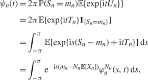
Proof. Indeed, since
 $$\int_{ - \pi }^\pi {{\rm{e}}^{{\rm{i}}s({S_n} - {m_n})}}{\rm{d}}s = 2\pi {1_{\{ {S_n} = {m_n}\} }},$$
we have
 $$\matrix{
{{\psi _n}(t) = 2\pi {\rm{\mathbb P}}({S_n} = {m_n}){\rm{\mathbb E}}[\exp \{ {\rm{i}}t{U_n}\} ]} \cr
{ = 2\pi {\rm{\mathbb E}}[\exp \{ {\rm{i}}t{T_n}{{\} 1}_{\{ {S_n} = {m_n}\} }}]} \cr
{ = \int_{ - \pi }^\pi {\rm{\mathbb E}}[\exp \{ {\rm{i}}s({S_n} - {m_n}) + {\rm{i}}t{T_n}\} ]{\rm{d}}s} \cr
{ = \int_{ - \pi }^\pi {{\rm{e}}^{ - {\rm{i}}s({m_n} - {N_n}{\rm{\mathbb E}}[{X_n}])}}\varphi _n^{{N_n}}(s,t){\rm{d}}s,} \cr
} $$
which leads to (15) after the change of variable 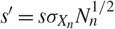 $s' = s{\sigma _X}_{_n}N_n^{1/2}.$.
Now we give controls on the function φn and its partial derivatives (see Lemmas 2 and 3).
Lemma 2. Under (A7), for any integer l ≥ 0,  $|s| \le \pi {\sigma _{{X_n}}}N_n^{1/2}$, and
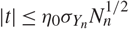 $|t| \le {\eta _0}\sigma {Y_n}N_n^{1/2}$, we obtain
 $$\left| {\varphi _n^{{N_n} - l}\left( {{s \over {{\sigma _{{X_n}}}N_n^{1/2}}},{t \over {{\sigma _{{Y_n}}}N_n^{1/2}}}} \right)} \right| \le {{\rm{e}}^{ - ({s^2} + {t^2}).{c_7}.({N_n} - l)/{N_n}}}.$$
Proof. The proof is a mere consequence of the inequality 1 + x ≤ ex that holds for any x ∈ ℝ.
Lemma 3. For any s and t, we have
 $$\left| {{{\partial {\varphi _n}} \over {\partial t}}\left( {{s \over {{\sigma _{{X_n}}}N_n^{1/2}}},{t \over {{\sigma _{{Y_n}}}N_n^{1/2}}}} \right)} \right| \le {{{\sigma _{{Y_n}}}} \over {N_n^{1/2}}}(|s| + |t|)$$
and
 $$\matrix{
{\left| {{{\partial {\varphi _n}} \over {\partial t}}\left( {{s \over {{\sigma _{{X_n}}}N_n^{1/2}}},{t \over {{\sigma _Y}_{_n}N_n^{1/2}}}} \right)} \right|} \hfill \cr
{\quad \quad \le {{{\sigma _{{Y_n}}}} \over {N_n^{1/2}}}|t| + {{\sigma {Y_n}} \over {{N_n}}}\left[ {{{{s^2}} \over 2}{{\left( {{{\rho {X_n}} \over {\sigma {X_n}^3}}} \right)}^{2/3}}{{\left( {{{\rho {Y_n}} \over {{\sigma _Y}{{_{_n}}^3}}}} \right)}^{1/3}} + |st|{{\left( {{{\rho {X_n}} \over {{\sigma _X}{{_{_n}}^3}}}} \right)}^{1/3}}{{\left( {{{\rho {Y_n}} \over {{\sigma _Y}{{_{_n}}^3}}}} \right)}^{2/3}} + {{{t^2}} \over 2}\left( {{{\rho {Y_n}} \over {\sigma {Y_n}^3}}} \right)} \right].} \hfill \cr
} $$
Proof. We apply Taylor’s theorem to the function defined by
 $$(s,t) \mapsto f(s,t) = {{\partial {\varphi _n}} \over {\partial t}}\left( {{s \over {{\sigma _{{X_n}}}N_n^{1/2}}},{t \over {{\sigma _{{Y_n}}}N_n^{1/2}}}} \right).$$
We obtain (17) using
 $$|f(s,t) - f(0,0)| \le |s|\mathop {\sup }\limits_{\theta ,\theta ' \in \left[ {0,1} \right]} \left| {{{\partial f} \over {\partial s}}(\theta s,\theta 't)} \right| + |t|\mathop {\sup }\limits_{\theta ,\theta ' \in \left[ {0,1} \right]} \left| {{{\partial f} \over {\partial t}}(\theta s,\theta 't)} \right|$$
and (18) using
 $$\matrix{
{|f(s,t) - f(0,0)| \le |s|\left| {{{\partial f} \over {\partial s}}(0,0)} \right| + |t|\left| {{{\partial f} \over {\partial t}}(0,0)} \right| + {{{s^2}} \over 2}\mathop {\sup }\limits_{\theta ,\theta ' \in \left[ {0,1} \right]} \left| {{{{\partial ^2}f} \over {{\partial ^2}s}}(\theta s,\theta 't)} \right|} \cr
{\quad {\kern 1pt} + |st|\mathop {\sup }\limits_{\theta ,\theta ' \in \left[ {0,1} \right]} \left| {{{{\partial ^2}f} \over {\partial t\partial s}}(\theta s,\theta 't)} \right| + {{{t^2}} \over 2}\mathop {\sup }\limits_{\theta ,\theta ' \in \left[ {0,1} \right]} \left| {{{{\partial ^2}f} \over {{\partial ^2}t}}(\theta s,\theta 't)} \right|.} \cr
} $$
The partial derivatives of f are estimated by mixed moments of Xn and Yn and then bounded above by Hölder’s inequality.
The following lemma is a result due to Quine and Robinson [Reference Quine and Robinson17, Lemma 2].
Lemma 4. Define
 $${l_{1,n}}: = {\rho _X}_{_n}{\sigma _X}{_{_n}^{ - 3}}N_n^{ - 1/2}\quad {\rm{and}}\quad {l_{2,n}}: = {\rho _Y}_{_n}{\sigma _Y}{_{_n}^{ - 3}}N_n^{ - 1/2}.$$
If l 1,n ≤ 12−3/2 and l 2,n ≤ 12−3/2, then, for all
 $$(s,t) \in R\mathop :\limits_ = \left\{ {(s,t):|s| < {\textstyle{2 \over 9}}l_{1,n}^{ - 1},|t| < {\textstyle{2 \over 9}}l_{2,n}^{ - 1}} \right\},$$
we have
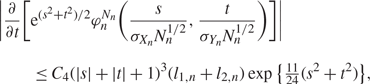 $$\matrix{
{\left| {{\partial \over {\partial t}}\left[ {{{\rm{e}}^{({s^2} + {t^2})/2}}\varphi _n^{{N_n}}\left( {{s \over {{\sigma _{{X_n}}}N_n^{1/2}}}} \right)} \right]} \right|} \hfill \cr
{\quad \quad \le {C_4}{{(|s| + |t| + 1)}^3}({l_{1,n}} + {l_{2,n}})\exp \{ {\textstyle{{11} \over {24}}}({s^2} + {t^2})\} ,} \hfill \cr
} $$
with C 4: = 161.
Remark 3. We make explicit the constant C 4 appearing at the end of the proof of Lemma 2 of [Reference Quine and Robinson17]. For all ν and s in R 2 as defined in [Reference Quine and Robinson17], we have
 $${{(|v| + 2|s|)} \over {{{(|v| + |s| + 1)}^3}({\ell _{1,n}} + {\ell _{2,n}})}}{e^{ - ({v^2} + {s^2})/24}} \le 108 \cdot \sqrt 6 { \cdot ^{ - 1/2}} \le 161.$$
By (A2) and (A3),
 $${l_{1,n}} \le N_n^{ - 1/2} \le {c_2}{c_3}\sigma _{{X_n}}^{ - 1/2}N_n^{ - 1/2},$$
which implies that 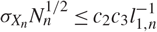 ${\sigma _{{X_n}}}N_n^{1/2} \le {c_2}{c_3}l_{1,n}^{ - 1}.$. Similarly,
 $${l_{2,n}} \le {c_5}N_n^{ - 1/2} \le {c_4}{c_5}{\sigma _{Yn}}^{ - 1}N_n^{ - 1/2},$$
and 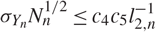 $\sigma {Y_n}N_n^{1/2} \le {c_4}{c_5}l_{2,n}^{ - 1}.$. Now we are able to establish (11).
Lemma 5. There exists a positive constant C 1, depending only on c 3, c 5, and c 1 such that, for  ${N_n} \ge {12^3}\max ({c_3}^2,{c_5}^2),$,
 $$\int_0^{\eta \sigma {Y_n}N_n^{1/2}} \mathop {\sup }\limits_{0\theta u} \,{I_1}(n,u,\theta ){\rm{d}}u \le {{{C_1}} \over {N_n^{1/2}}}.$$
Proof. The definitions of η in (7) and ε in (8) imply that, for s ∈ A 1 and u and θ as in the integral in the statement above, we have
 $$|s| < \varepsilon {\sigma _{{X_n}}}N_n^{1.2} \le {\textstyle{2 \over 9}}l_{1,n}^{ - 1}\quad {\rm{and}}\quad |\theta | \le |u| \le \eta {\sigma _{{Y_n}}}N_n^{1/2} \le {\textstyle{2 \over 9}}l_{2,n}^{ - 1},$$
which ensures that (s, θ) ∈ R as specified in Lemma 4. Moreover, for  ${N_n} \ge {12^3}\max ({c_3}^2,{c_5}^2),$, l 1,n ≤ 12-3/2 and l 2,n ≤ 12-3/2. Now using Lemma 4 in (9) and by (A1), we get
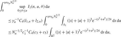 $$\matrix{
{\int_0^{\eta \sigma {Y_n}N_n^{1/2}} \mathop {\sup }\limits_{0\theta u} {I_1}(n,u,\theta ){\rm{d}}u} \hfill \cr
{\quad \quad \le {\gamma _n}^{ - 1}{C_4}({l_{1,n}} + {l_{2,n}})\int_0^{\eta \sigma {Y_n}N_n^{1/2}} \int_{{A_1}} (|s| + |u| + 1){{\rm{e}}^3}^{ - ({s^2} + {u^2})/24}{\rm{d}}s\,{\rm{d}}u} \hfill \cr
{\quad \quad \le N{{_n^{ - 1/2}}^{ - 1}}c_1^{ - 1}{C_4}({c_3} + {c_5})\int_{{{\rm{\mathbb R}}^2}} {{(|s| + |u| + 1)}^3}{{\rm{e}}^{ - ({s^2} + {u^2})/24}}{\rm{d}}s\,{\rm{d}}u,} \hfill \cr
} $$
and the result follows with
 $${C_1}: = {c_1}^{ - 1}{C_4}({c_3} + {c_5})\int_{{{\rm{\mathbb R}}^2}} {(|s| + |u| + 1)^3}{{\rm{e}}^{ - ({s^2} + {u^2})/24}}{\rm{d}}s\,{\rm{d}}u.$$
Remark 4. Actually, Lemma 5 is valid as soon as  $N_n \ge \max (c_3^2, c_5^2 )$: the constants in the proof of Lemma 2 of [Reference Quine and Robinson17] can be improved.
Now we are able to prove (12).
Lemma 6. There exists a positive constant C 2, depending only on c 1, c̃ 2, c 2, c 3, and c 7 such that, for Nn ≥ 2,
 $$\int_0^{\eta {\sigma _{{Y_n}}}N_n^{1/2}} {\mathop {\sup }\limits_{0 \le \theta \le u} } {I_2}(n,u,\theta ){\rm{d}}u \le {{{C_2}} \over {N_n^{1/2}}}.$$
Proof. We use the controls (16) with t = θ and l = 1, (17), and |φn| ≤ 1 to get
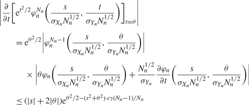 $$\matrix{
{\left| {{\partial \over {\partial t}}{{\left[ {{{\rm{e}}^{{t^2}/2}}\varphi _n^{{N_n}}\left( {{s \over {{\sigma _{{X_n}}}N_n^{1/2}}},{t \over {{\sigma _{{Y_n}}}N_n^{1/2}}}} \right)} \right]}_{t = \theta }}} \right|} \hfill \cr
{\quad \quad = {{\rm{e}}^{{\theta ^2}/2}}\left| {\varphi _n^{{N_n} - 1}\left( {{s \over {{\sigma _{{X_n}}}N_n^{1/2}}},{\theta \over {{\sigma _{{Y_n}}}N_n^{1/2}}}} \right)} \right|} \hfill \cr
{\quad \quad \quad {\kern 1pt} \times \left| {\theta {\varphi _n}\left( {{s \over {{\sigma _{{X_n}}}N_n^{1/2}}},{\theta \over {{\sigma _{{Y_n}}}N_n^{1/2}}}} \right) + {{N_n^{1/2}} \over {{\sigma _Y}_{_n}}}{{\partial {\varphi _n}} \over {\partial t}}\left( {{s \over {{\sigma _{{X_n}}}N_n^{1/2}}},{\theta \over {{\sigma _{{Y_n}}}N_n^{1/2}}}} \right)} \right|} \hfill \cr
{\quad \quad \le (|s| + 2|\theta |){{\rm{e}}^{{\theta ^2}/2 - ({s^2} + {\theta ^2}) \cdot {c_7}({N_n} - 1)/{N_n}}}} \hfill \cr
} $$
for s ∈ A2 and u and θ as in the integral in the statement of the lemma. Finally, using (10), we get, for Nn ≥2,
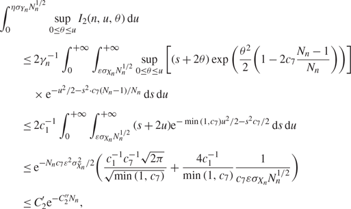 $$\eqalign{
& \int_0^\eta \mathop {\sup }\limits_{0\theta u} {I_2}(n,u,\theta )u \cr
& \matrix{
{\quad \quad \le {2^{ - 1}}\int_0^{ + \infty } \int_{\varepsilon XnN_n^{1/2}}^{ + \infty } \mathop {\sup }\limits_{0 \le \theta \le u} [(s + 2\theta )\exp ({{{\theta ^2}} \over 2}(1 - 2{{{N_n} - 1} \over {{N_n}}}))]} \hfill \cr
{\quad \quad \quad {\kern 1pt} \times {{\kern 1pt} ^{ - {u^2}/2 - {s^2} \cdot ({N_n} - 1)/{N_n}}}su} \hfill \cr
{\quad \quad \le {2^{ - 1}}\int_0^{ + \infty } \int_{\varepsilon XnN_n^{1/2}}^{ + \infty } {{(s + 2u)}^{ - \min (1,){u^2}/2 - {s^2}/2}}su} \hfill \cr
{\quad \quad { \le ^{ - {N_n}{\varepsilon ^2}X{n^2}/2}}({{{{^{ - 1}}^{ - 1}}\sqrt {2\pi } } \over {\sqrt {\min (1,)} {\kern 1pt} }} + {{{4^{ - 1}}} \over {\min (1,)}}{1 \over {\varepsilon XnN_n^{1/2}}})} \hfill \cr
{\quad \quad \le {C_{2'}}^{ - {C_{2''}}{N_n}},} \hfill \cr
} \cr} $$
where
 $$C_2^{'}: = {c_1}^{ - 1}{c_7}^{ - 1}\left( {{{\sqrt {2\pi } } \over {\sqrt {\min (1,{c_7})} {\kern 1pt} }} + {4 \over {\min (1,{c_7})\min ((2/9)({c_2}{c_3}{)^{ - 1}},\pi ){{\tilde c}_2}}}} \right)$$
and
 $$C_2^{''}: = {\tilde c_2}^2/2{c_7}\min {({\textstyle{2 \over 9}}{({c_2}{c_3})^{ - 1}},\pi )^2}.$$
The result follows, writing
 $$C_2^{'}{{\rm{e}}^{ - C_2^{''}{N_n}}} = {{C_2^{'}{{(C_2^{''})}^{ - 1/2}}} \over {N_n^{1/2}}}{({C_3}{N_n})^{1/2}}{{\rm{e}}^{ - {C_3}{N_n}}} \le {{C_2^{'}{{(C_2^{''})}^{ - 1/2}}} \over {N_n^{1/2}}}{(1/2)^{1/2}}{e^{ - 1/2}} = :{\kern 1pt} {{{C_2}} \over {N_n^{1/2}}},$$
since x 1/2e-x is maximum in  ${1 \over 2}$.


