Nomenclature
 ${a_{t,i}}$
action assigned to tail number
$i$ at timestep $t$- ${{{\mathord{\buildrel{\lower3pt\hbox{$\scriptscriptstyle\rightharpoonup$}}\over A}}_t}}$
action vector
- $b$
body width in metres
- $C$
Paris coefficient
- ${d_{t,i}}$
damage level at time
$t$ for tail number $i$- ${f_0}$
cyclic stress frequency in Hz
- $m$
Paris exponent
- ${M_i}$
mission type
- MADDPG
multi-agent deep deterministic policy gradient
- MDP
Markov decision process
- MT
(preventative) maintenance
- O&M
operations and maintenance
- ${P_{sa\;}}$
state transition probabilities
- $Q( {{{\mathord{\buildrel{\lower3pt\hbox{$\scriptscriptstyle\rightharpoonup$}}\over S} }_t},{{\mathord{\buildrel{\lower3pt\hbox{$\scriptscriptstyle\rightharpoonup$}}\over A} }_t}} )$
value of action
${{{\mathord{\buildrel{\lower3pt\hbox{$\scriptscriptstyle\rightharpoonup$}}\over A} }_t}}$ in state ${{{\mathord{\buildrel{\lower3pt\hbox{$\scriptscriptstyle\rightharpoonup$}}\over S} }_t}}$- $R( {{{\mathord{\buildrel{\lower3pt\hbox{$\scriptscriptstyle\rightharpoonup$}}\over S} }_t},{{\mathord{\buildrel{\lower3pt\hbox{$\scriptscriptstyle\rightharpoonup$}}\over A} }_t}})$
reward obtained for taking action
${{{\mathord{\buildrel{\lower3pt\hbox{$\scriptscriptstyle\rightharpoonup$}}\over A} }_t}}$ in state ${{{\mathord{\buildrel{\lower3pt\hbox{$\scriptscriptstyle\rightharpoonup$}}\over S} }_t}}$- RL
reinforcement learning
- SB
standby
- ${{{\mathord{\buildrel{\lower3pt\hbox{$\scriptscriptstyle\rightharpoonup$}}\over S} }_t}}$
state vector
- $x\!\left( t \right)$
crack length in metres at timestep
$t$


Greek symbols
- $\alpha $
learning rate
- $\gamma $
discount factor
- ${{\rm{\Delta }}_\sigma }$
stress range in MPa
- $\Delta t$
interval between of time between
$t$ and $t + 1$- $\Delta x$
change in crack length
- $\varepsilon $
exploration rate
- ${\varepsilon _{max}},\;{\varepsilon _{min}}\;$
maximum and minimum exploration rate
- ${\varepsilon _{decay}}$
decay of exploration rate
- ${\mu _i}$
manoeuvre type


1.0 Introduction
A fleet of aircraft can be seen as a set of degrading systems that undergo variable loads as they fly missions and require maintenance throughout their lifetime. Aircraft fleet management aims to maximise fleet availability while minimising maintenance costs. To achieve this goal, individual aircraft, with variable age and degradation paths, need to operate cooperatively to maintain high fleet availability while avoiding mechanical failure by scheduling preventive maintenance actions. Therefore, decision planning for an efficient fleet management is crucial to ensure fleet availability, reliability and reduce maintenance costs [Reference Painter, Erraguntla, Hogg and Beachkofski1, Reference Khoo and Teoh2]. Yet, aircraft fleet management is a very complex decision-making problem with a large number of degrees of freedom, as operators need to decide for each tail number whether to fly a mission, stand-by or go under maintenance. Finding an optimal solution to this problem is non-trivial.
In recent years, reinforcement learning (RL) has emerged as an effective optimisation method for complex decision-making problems. RL is a machine learning technique suitable to solve sequential decision-making problems and it has had success in many applications including autonomous driving [Reference Kiran, Sobh, Talpaert, Mannion, Al Sallab, Yogamani and Pérez3], inventory management [Reference Giannoccaro and Pontrandolfo4] and game artificial intelligence [Reference Silver, Hubert and Schrittwieser5]. It distinguishes itself from supervised learning in many ways. While in supervised learning we provide examples to our models from which they can learn how to match the inputs to exact outputs (labels or numeric values), when dealing with a sequential decision-making problem it becomes very challenging to provide explicit supervision. Instead, in RL we provide the algorithms with a reward function and let the agent explore the different state-action pairs and learn from experience, in a process that is referred to as ‘self-play’ [Reference Sutton and Barto6]. During self-play the agent randomly explores the actions in a simulated environment, formulated as a Markov decision process (MDP), and iteratively learns the sequence of actions that lead to maximum rewards.
Given the importance of maintenance management in many industrial applications, a growing body of literature has focused on developing optimisation frameworks, RL and non-RL (e.g., Monte Carlo simulations, linear programming etc.), for the operation and maintenance (O&M) of mechanical components. While a significant body of work has focused on simulation/optimisation frameworks to solve the maintenance task scheduling problem of a fleet of aircraft [Reference Mattila and Virtanen7–Reference Marlow, Looker and Mukerjee10], in this work we will mainly focus on previous RL applications. Several recent studies [Reference Bellani, Compare, Baraldi and Zio11, Reference Lee and Mitici12] proposed novel RL frameworks to optimise the O&M of a single mechanical component (e.g., pump/turbine/turbofan engine) and demonstrated that it can find optimal policies when compared to traditional maintenance strategies. However, when considering an entire fleet of aircraft, there is not a single component to optimise but multiple components must be operated simultaneously and cooperatively to reach a common goal, maximising the overall availability of the fleet and minimising the cost of maintaining the fleet. This multi-component optimisation drastically increases the difficulty (i.e., degrees of freedom) of the decision-making problem. For instance, [Reference Yousefi, Tsianikas and Coit13] used RL to optimise the maintenance scheduling of a system with three individually repairable components, but extending this framework to more components rapidly becomes computationally intractable. To overcome this combinatorial explosion, where the computational space exponentially increases with the number of components, different approaches have been employed in the literature. For a manufacturing process with multiple repairable machines, Ref. [Reference Kuhnle, Jakubik and Lanza14] suggested to break down the system by assigning one RL agent per machine. Another way of restricting the computational space is observed in Ref. [Reference Mattila and Virtanen15], the only other study to our knowledge that attempts to use RL to optimise the maintenance scheduling of a fleet of aircraft. In Ref. [Reference Mattila and Virtanen15], however, only the most damaged tail number in the fleet is considered by the RL agent at each timestep, instead of making decisions for each aircraft in the fleet, which drastically reduces the complexity of the problem. Although both methods manage to considerably decrease the computational space of the problem, they come at a price of losing information related to the state of the fleet and potentially not capturing the optimal collaborative behaviour of each component in order to achieve overall fleet availability.
This article aims to develop a comprehensive RL framework for aircraft fleet availability optimisation that considers both mission assignment and maintenance scheduling. A degradation model is combined with flight missions and maintenance actions to design an environment (i.e. MDP) that simulates the operation of a fleet of aircraft, with variable age and degradation paths, over their lifetime. The goal of the RL algorithm is to find a sequence of actions (policy) that maximises the number of missions completed by the fleet while minimising the maintenance costs, and doing so, outperforms a set of baseline policies derived from traditional O&M strategies.
The manuscript is organised as follows. Section 2.0 presents the simulated environment that describes the logic of the fleet O&M, including a degradation model based on the Virkler fatigue crack propagation experimental dataset [Reference Virkler, Hillberry and Goel16] (Section 2.1), a set of flight manoeuvres and missions (Section 2.2) and preventive and corrective maintenance actions (Section 2.3). Section 3.0 describes the RL framework, which uses an MDP and a Q-learning algorithm. Section 4.0 presents three case studies with fleets that have an increasing number of aircraft (2, 3 and 4, respectively) and compares the resulting RL policies against baseline strategies. Section 5.0 discusses the results and potential applications of this work and highlights the limitations and areas of improvement for future work.
2.0 Simulated enviroment
This section describes the mathematical formulation that was designed to simulate the O&M of a fleet of aircraft, including mission assignment and maintenance scheduling.
2.1 Degradation model
The maintenance of aircraft can be driven by multiple factors, such as corrosion damage, fatigue crack damage and aircraft usage [Reference Findlay and Harrison17]. Assuming the driving factor for aircraft maintenance is the cracking damage at the critical locations of the airframe structure (e.g., the wing root), a model describing the propagate of a crack was used to simulate aircraft damage. The degradation was designed to follow a Paris’ law [Reference Paris and Erdogan18] and replicate the degradation paths observed in the Virkler experiment [Reference Virkler, Hillberry and Goel16]. The crack length propagation is described by the following equation:
 \begin{align}x\!\left( {t + \;{\rm{\Delta }}t} \right) = C\;{f_0}{\rm{\;\Delta }}t{\left( {{{\rm{\Delta }}_\sigma }\sqrt {\frac{{\;\pi \;x\!\left( t \right)}}{{\cos \!\frac{{\pi \;x\!\left( t \right)}}{{2b}}}}} } \right)^m}\end{align}
where  $x\!\left( {t + \;{\rm{\Delta }}t} \right)$ is the new crack length after a period
 ${\rm{\Delta }}t$,
 ${f_0}$ the cyclic stress frequency (in Hz),
 $C$ the Paris coefficient,
 $m$ the Paris exponent,
 $\;{{\rm{\Delta }}_\sigma }$ the stress range (in MPa),
 $b$ the body width (in metres) and
 $x\!\left( t \right)$ the initial crack length (in metres).
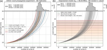
Each tail number in the fleet is assigned a different C coefficient drawn from a normal distribution (with mean 8.586e–11 and standard deviation 0.619e–11). The Paris exponent  $m$ is set to 2.9. These parameters of the degradation model were calibrated to reproduce the degradation paths observed during the Virkler experiment [Reference Virkler, Hillberry and Goel16], based on 68 replicate crack propagation tests of aluminium alloy panels under constant load and environmental conditions run to failure during a large number of cycles (N). In the Virkler experiment, the initial crack length was 9 mm and the body width (
 $b$) 76.2 mm, the tests were stopped when the crack length reached 50 mm. Figure 1 shows the similarity between the experimental degradation paths in the Virkler dataset (Fig. 1a) and degradation model described above (Fig. 1b).
(a) Degradation paths for the 68 replicates in the Virkler fatigue crack propagation experiment [Reference Virkler, Hillberry and Goel16]. (b) Degradation model as described in Equation 1) using a stress range  ${\rm{\;}}{{\rm{\Delta }}_{\rm{\sigma }}}$ = 48.26 MPa and Paris exponent m = 2.9. The degradation paths are plotted for 68 Paris coefficients (C in Equation 1) drawn from a normal distribution with mean 8.586e–11 and standard deviation 0.619e–11. N is the number of cycles with constant load over which the crack propagates.

The crack length was discretised into 10 equally spaced bins between the initial crack length (9 mm) and half the body width of the aluminium alloy panels (38.1 mm), hereafter referred to as ‘damage levels’ and shown in Fig. 1b. The failure threshold was set to 50% of the body width to ensure an ample margin of safety. When the crack length surpasses the failure threshold, the aircraft must undergo repairs before it can resume operation.
2.2 Aircraft manoeuvres and missions
While the Paris coefficients ( $C$ values) are drawn randomly for each aircraft in the fleet and then used throughout their lifetime, the stress range (
 $\;{{\rm{\Delta }}_\sigma }$) varies depending on the manoeuvre that the aircraft performs. Five manoeuvres that an aircraft can perform were designed based on expert input and are described in Table 1, note that these numbers are indicative and only useful for the purpose of this synthetic environment (not to be referenced as ground truth). Subsequently, mission types were designed by combining each manoeuvre over a varying length of time. While a wide range of mission types may be completed by the aircraft in real-word scenarios, here it was simplified by designing two mission types with varying degree of difficulty. The manoeuvre composition of the two missions,
 ${M_1}$ and
 ${M_2}$, is reported in Table 2. Mission 1 consists of 2,600 seconds of level fly (
 ${\mu _1}$), 60 seconds for take-off and landing (
 ${\mu _2}$), 30 seconds of barrel rotate (
 ${\mu _3}$) and 10 seconds of vertical up/down (
 ${\mu _5}$). On the other hand, Mission 2 consists of 4,500 seconds of level fly (
 ${\mu _1}$), 60 seconds for take-off and landing (
 ${\mu _2}$), 60 seconds of pull up/down (
 ${\mu _4}$) and 80 seconds of vertical up/down (
 ${\mu _5}$). A cyclic stress frequency
 ${f_0}$ of 5 Hz is used to propagate the crack length for the duration of each manoeuvre. We need to emphasise that this synthetic environment for aircraft operation is not necessarily representational in the real world but the principle of applying the RL to an environment of aircraft operation is the same.
Manoeuvres and missions

Mission types

Equation (1) can now be reformulated to calculate the crack propagation resulting from a tail number flying one of the two missions:
 \begin{align}\Delta {x_i}\!\left( {t,\;{M_j}} \right) = {C_i}\;{f_0}\mathop \sum \nolimits_{k = 1}^{k = 5} \Delta t\!\left( {{\mu _k}} \right){\left[ {\Delta \sigma\!\left( {{\mu _k}} \right)\sqrt {{{\;\pi \;{x_i}\!\left( t \right)} \over {\cos {{\pi \;{x_i}\!\left( t \right)} \over {2b}}}}} } \right]^m}\end{align}
where  $\Delta {x_i}\!\left( {t,\;{M_j}} \right)$ is the crack length propagation for tail number
 $i$ at timestep
 $t$ after completing mission
 ${M_j}$.
 $\Delta t(\mu_{k})$ and
 $\Delta \sigma(\mu_{k})$ are taken from Table 2 based on the selected mission (
 ${M_1}$ or
 ${M_2}$). A set of missions is prescribed daily to the fleet, and each tail number can either fly one of the prescribed missions.
2.3 Preventive and corrective maintenance
As the tail numbers fly the prescribed missions, they accumulate damage, and to continue operating, maintenance is required. Each tail number can be sent to preventive maintenance at any time during its lifetime. When the tail number is under maintenance it becomes unavailable for a period of time and its damage level is restored to the initial crack length (9 mm). However, if the tail number is not sent to preventive maintenance in time and its damage level goes above the failure threshold (38.1 mm, as the specimen width b = 76.2 mm in the Virkler experiment), the tail number automatically goes to corrective maintenance, which has a much higher cost than preventive maintenance. Arbitrarily, the costs of preventive and corrective maintenance are set to 10 and 100 respectively, and in both cases the tail number becomes unavailable for a week, after which it can resume operation.
3.0 Reinforcement learning framework
3.1 Markov decision processes
An MDP is the formalism to describe sequential decision making and is adopted in RL problems. As defined in Ref. [Reference Sutton and Barto6], an MDP is a tuple with five variables (  $\mathord{\buildrel{\lower3pt\hbox{$\scriptscriptstyle\rightharpoonup$}} \over S} \;$,
 $\mathord{\buildrel{\lower3pt\hbox{$\scriptscriptstyle\rightharpoonup$}} \over A} \;$,
 ${P_{sa\;}}$,
 $R$,
 $\gamma $) where:
•
$\mathord{\buildrel{\lower3pt\hbox{$\scriptscriptstyle\rightharpoonup$}} \over S} $ is a set of states that the agent observes (e.g., damage level of each aircraft in the fleet).-
•
$\mathord{\buildrel{\lower3pt\hbox{$\scriptscriptstyle\rightharpoonup$}} \over A} $ is a set of actions (e.g., fly a mission, stand-by or apply preventive maintenance). -
•
${P_{sa}}$ are the state transition probabilities, which give the probability of transitioning to each other state when taking action a in state s. -
•
$R$ is the reward function which maps each state-action pair to a reward value. -
•
$\gamma $ is the discount factor, a value between 0 and 1 used to discount future rewards.


In the dynamics of an MDP, we start in a certain state  ${s_0}$, choose action
 ${a_0}$, randomly transition to the next state
 ${s_1}$ and receive reward
 $R\!\left( {{s_0},{a_0}} \right)$, then choose another action
 ${a_1}$ and transition to state
 ${s_2}$ and receive reward
 $R\!\left( {{s_1},{a_1}} \right)$, and so on and so forth:
 \begin{align}{s_0}\;\begin{array}{*{20}{c}}{{a_0}}\\{ - - - - - \; \to \;}\\{R\!\left( {{s_0},{a_0}} \right)}\end{array}\;{s_1}\;\begin{array}{*{20}{c}}{{a_1}}\\{ - - - - - \; \to \;{s_2}\;}\\{R\!\left( {{s_1},{a_1}} \right)}\end{array}\begin{array}{*{20}{c}}{{a_2}}\\{ - - - - - \; \to \;}\\{R\!\left( {{s_2},{a_2}} \right)}\end{array}\;\;.\;\;.\;\;.\end{align}
The goal of RL algorithms is to choose the sequence of actions that maximise the expected value of the total payoff, which is the immediate reward plus the sum of future discounted rewards:
 \begin{align}E\!\left[ {R\!\left( {{s_0},{a_0}} \right) + \gamma R\!\left( {{s_1},{a_1}} \right) + \;{\gamma ^2}R\!\left( {{s_2},{a_2}} \right) + \;.\;\;.\;\;.\;} \right]\end{align}
The function that maps the states to the actions  $\pi :\;\mathord{\buildrel{\lower3pt\hbox{$\scriptscriptstyle\rightharpoonup$}} \over S} \to \mathord{\buildrel{\lower3pt\hbox{$\scriptscriptstyle\rightharpoonup$}} \over A} $ is referred to as a policy. While there are no universal methods for searching the optimal policy, popular approaches include dynamic programming (value iteration and policy iteration), Monte-Carlo methods and time-difference methods (e.g., Q-learning) [Reference Sutton and Barto6]. While some methods like dynamic programming require a model of the environment (i.e. known state transition probabilities
 ${P_{sa}}$), other methods are model-free and do not require prior knowledge of the state transition probabilities. In this case, the state transition probabilities
 ${P_{sa}}$ are not known so it was decided to use Q-learning [Reference Watkins and Dayan19], a model-free RL algorithm.
3.2 States and actions
The State vector ( ${\mathord{\buildrel{\lower3pt\hbox{$\scriptscriptstyle\rightharpoonup$}}\over S} _t}$) contains the observed variables, which track the damage level (discrete values) of each tail number in the fleet at each point in time. The Action vector (
 ${\mathord{\buildrel{\lower3pt\hbox{$\scriptscriptstyle\rightharpoonup$}}\over S} _t}$) contains the decision chosen by the RL agent at each timestep, which includes one action for each tail number in the fleet. For a fleet of
 $n\;$aircraft, they are defined as follows:
 \begin{align}{\mathord{\buildrel{\lower3pt\hbox{$\scriptscriptstyle\rightharpoonup$}}\over S} _t} = \left[ {{d_{t,1}}\;\;\;\;{d_{t,2}}\;\; \ldots \;\;{d_{t,n}}} \right],\quad {\mathord{\buildrel{\lower3pt\hbox{$\scriptscriptstyle\rightharpoonup$}}\over S} _t} \in {\mathbb N}^{n}\end{align}
where  ${d_{t,i}} \in \left\{ {1,\; \ldots ,\;9} \right\}$ is the damage level of tail number
 $i$ at timestep
 $t$ and
 $n$ is the number of aircraft in the fleet.
 \begin{align} {\mathord{\buildrel{\lower3pt\hbox{$\scriptscriptstyle\rightharpoonup$}}\over A} _t} = \left[ {{a_{t,1}}\;\;\;\;{a_{t,2}}\; \ldots \;\;{a_{t,n}}} \right],\quad {\mathord{\buildrel{\lower3pt\hbox{$\scriptscriptstyle\rightharpoonup$}}\over A} _t} \in {\mathbb N}^{n}\end{align}
where  ${a_{t,i}}$ is the action assigned to tail number
 $i$ at timestep
 $t$. The action
 ${a_{t,i}}$ can take one of four possible values depending on whether the tail number is assigned one of the two missions, put in standby or sent to preventive maintenance:
 \begin{align}{a_{t,i}} = \left\{ {\begin{array}{l@{\quad}l}0&{{\rm{fly\;}}{{\rm{M}}_1}}\\[5pt] 1&{{\rm{fly\;}}{{\rm{M}}_2}}\\[5pt] 2&{{\rm{standby\;}}\left( {{\rm{SB}}} \right)}\\[5pt] 3&{{\rm{preventive\;maint}}.{\rm{\;}}\left( {{\rm{MT}}} \right)}\end{array}} \right.\end{align}
Hence, at each timestep the RL agent must choose one out of  ${4^n}$ possible decisions.
The following logic is used when an action is chosen in each state:
i. if a tail number is assigned a mission (
${M_1}$ or ${M_2}$), its damage level is updated using Equation (2)a. if the new damage level after flying a mission is above the failure threshold, the tail number is automatically sent to corrective maintenance: the tail number is unavailable for one week and its damage level is restored to the initial damage (9 mm crack length).
-
ii. if a tail number is under preventive maintenance, the tail number becomes unavailable to fly missions for one week after which its damage level is restored to the initial damage.
-
iii. if standby is chosen, the damage level remains unchanged.


3.3 Rewards
The Reward function  $R( {{{\mathord{\buildrel{\lower3pt\hbox{$\scriptscriptstyle\rightharpoonup$}}\over S} }_t},{{\mathord{\buildrel{\lower3pt\hbox{$\scriptscriptstyle\rightharpoonup$}}\over A} }_t}})$ is designed to help the agent achieve its goal by incentivising certain actions. It is defined as follows:
 \begin{align}R( {{{\mathord{\buildrel{\lower3pt\hbox{$\scriptscriptstyle\rightharpoonup$}}\over S} }_t},{{\mathord{\buildrel{\lower3pt\hbox{$\scriptscriptstyle\rightharpoonup$}}\over A} }_t}\;}) =
\left\{ \begin{array}{l@{\quad}l} + 1 & \textrm{for\;completing}\; {{\rm{M}}_1} \\[5pt] + 2 & \textrm{for\;completing}\;{{\rm{M}}_2} \\[5pt] - 1 & \textrm{for\;standby} \\[5pt] - 10 & \textrm{preventive\;maint.}\\[5pt] - 100 & \textrm{corrective\;maint.} \end{array}\right.
\end{align}
This reward scheme encourages the agent to fly missions and send aircraft to preventive maintenance before they reach the failure threshold, as corrective maintenance costs 10 times more than acting preventively.
3.4 Q-learning
Q-learning is a model-free algorithm that has been widely used to find the optimal policy in finite discrete MDPs [Reference Clifton and Laber20]. The ‘Q’ in Q-learning stands for ‘quality’, which represents the value of taking a particular action in a particular state. Specifically, the Q-value of a state-action pair,  $Q( {\overrightarrow {{S_t}} ,\overrightarrow {{A_t}} } )$, is the expected total reward that an agent will receive starting from that state, taking that action and following the optimal policy thereafter. Q-learning works by iteratively updating the Q-values based on the rewards received by the agent from the environment. Thereby it belongs to the category of temporal difference (TD) methods in which the difference in prediction over successive timesteps is used to drive the learning process. The agent explores the state-action pairs in the environment and calculates the expected rewards for an action taken in a given state using Bellman’s update [Reference Sutton and Barto6]:
 \begin{align}Q(\! {\overrightarrow {{S_t}} ,\overrightarrow {{A_t}} } ) \leftarrow \;Q(\! {\overrightarrow {{S_t}} ,\overrightarrow {{A_t}} } ) + \alpha [ {{R_{t + 1}} + \gamma \;\mathop {\max }\limits_a Q( {\overrightarrow {{S_{t + 1}}} ,a} ) - Q(\! {\overrightarrow {{S_t}} ,\overrightarrow {{A_t}} } )} ]\end{align}
where  $Q( {\overrightarrow {{S_t}} ,\overrightarrow {{A_t}} })$ represents the expected sum of future rewards for taking action
 $\overrightarrow {{A_t}} $ in state
 $\overrightarrow {{S_t}} $ (known as the Q-value or quality of the state action pair),
 $\alpha $ is the learning rate and
 $\gamma $ the discount factor. The Q-values for each state-action pair encountered are stored in a look-up table and updated throughout the search. The search is conducted by running ‘episodes’, which consist of operating the fleet for N decisions (e.g. five-year period) and iteratively updating the Q-values after each decision using Equation 9. To ensure that the state and action spaces are thoroughly explored, although not exhaustively, an epsilon-greedy search strategy is implemented, in which the agent initially explores the environment (by choosing random actions) and as it gains experience in the environment it gradually reduces the exploration rate and begins to exploit its knowledge (by choosing the action with highest Q-value). The exploration rate
 $\varepsilon$ is set to decay during the search according to the following equation:
 \begin{align}\varepsilon\! \left( k \right) = \;{\varepsilon _{min}} + \left( {{\varepsilon _{max}} - {\varepsilon _{{\rm{min}}}}} \right){e^{\left( { - {\varepsilon _{decay}}k} \right)}}\end{align}
where  $k$ is the number of episodes in the search,
 ${\varepsilon _{min}}$ and
 ${\varepsilon _{max}}$ respectively the minimum and maximum rates of exploration and
 ${\varepsilon _{decay}}$ the rate of decay. The learning rate,
 $\alpha $ in Equation 9, dictates by how much existing Q-values are updated with new observations. This parameter is also set to decay during the search according to Equation 10, to gradually decrease the magnitude of new updates and help with the convergence of the policy.
A pseudocode describing how the policy search was implemented is included in Table 3.
Algorithm pseudocode for RL policy optimisation.

4.0 Case studies
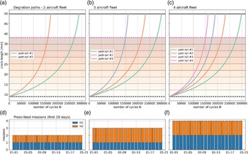
The RL framework for aircraft fleet management described above was tested on three case studies by applying it to optimise the operation of a fleet of respectively two, three and four aircrafts. Figure 2 depicts the fleet environment that was created for each case. At every timestep ( ${\rm{\Delta }}t$ = 1 day), a set of missions that matches the number of aircraft was prescribed to the fleet. The composition of the prescribed mission is kept constant throughout the lifetime of the fleet and is reported in Table 4. The epsilon and alpha decay curves and rewards obtained during the policy search as displayed in Fig. 3 for each case.
Illustration of the fleet environment for the three different case studies. Subplots (a), (b) and (c) show the degradation paths based on constant cycles for each aircraft in the fleet and (d), (e), and (f) display the missions prescribed to the fleet each given day.

Environment and search parameters for the three case studies

RL policy search for the three case studies and corresponding search parameters (exploration and learning rates). Subplots (a), (b) and (c) show the reward per episode achieve by the Q-table during the policy search and (d), (e), and (f) depict the decay curves for the exploration and learning rates. Note that the exploration rate has a minimum of 1% while the learning rate reaches a minimum of 10%.

To evaluate the performance of the resulting RL policies, two baseline strategies were designed based on established fleet management principles:
a) On-condition maintenance: in this policy preventive maintenance is assigned whenever an aircraft’s damage level goes above a fixed threshold. This threshold was optimised by trial-and-error, and it was found to provide the highest reward when set at a damage level of 8/10 (10 being the failure state). Outside of the maintenance zone, this policy assigns the prescribed missions randomly to the available aircraft.
-
b) Force-life management: in this policy, mission assignments are optimised to ensure smarter distribution of tasks. The missions are assigned in a manner that maintains the cumulated damage (i.e., crack length growth) equal across the fleet. This approach helps to maintain equal wear and tear on each aircraft, leading to improved efficiency and longevity of the fleet. Preventive maintenance is applied according to the on-condition maintenance strategy, when damage level goes above a damage level of 8.
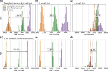
The RL policy was evaluated against the baseline strategies by running 10,000 episodes of five-year with each policy, with each episode starting with random initial conditions. Figure 4 shows the distribution of the rewards obtained by each policy, as well as the distribution of the runs that are located below the fifth percentile, which correspond to the worst-case scenarios out of the 10,000 cases. The results are also reported in Table 5.
Evaluation of the performance of the RL policy by comparing the average reward and fifth percentile from 10,000 episodes with random initial conditions; the highest reward displayed in bold

*% difference compared to on-condition maintenance.
Evaluation of the reinforcement learning policy against baseline strategies (on-condition maintenance and force-life management). Subplots (a), (b) and (c) show the distribution of the rewards over 10,000 episodes the two-, three- and four-aircraft environments respectively, with subplots (d), (e) and (f) indicating the rewards below the fifth percentile of the distributions, which indicate the worst-case scenarios. The percentage difference between RL policy and on-condition maintenance is indicated by an arrow.

For the two-aircraft environment, the average reward obtained with the RL policy is 10% higher than the on-condition policy (fixed maintenance and random mission assignment), and about 3% higher than force-life management (Fig. 4a), which demonstrates that the RL framework was capable of successfully optimising this problem. For the three-aircraft problem, the RL policy outperformed both on-condition maintenance and force-life management strategies by an even higher margin, showing improvements of 12% and 5% (Fig. 4b), respectively. Yet, this performance could not be recreated for the four-aircraft fleet, where the RL policy slightly outperforms the baseline policies by 4.1% (Fig. 4c). While the average reward from the distribution provides an indication of the performance of each policy, from a decision-making perspective, considering the worst-case scenario rather than the average case is more meaningful. Thus, Fig. 4 also shows the location of the fifth percentile of each distribution and the part that is located below it, which indicates the worst-case scenarios out of the 10,000 simulations. For the 2two- and three-aircraft fleets, the distributions have a small spread, therefore the performance evaluated with the fifth percentile matches with the average reward. However, in the four-aircraft fleet, the on-condition maintenance strategy and RL policy have a longer tail, which indicates that there are certain initial conditions for which they do not perform well. The reward distribution of the RL policy is skewed and thus the fifth percentile only outperforms on-condition maintenance by 2.4% and underperforms force-life management by 3.5%.
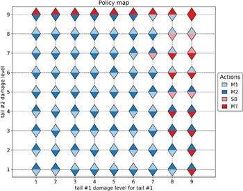
Policy map for the two-aircraft fleet showing the preferred action in each possible state. The bottom triangle shows the action assigned to tail #1 while the top one is for tail #2.

5.0 Discussion
5.1 Interpretability of RL policy
The policy obtained with the RL framework presented here was able to outperform the baseline strategies for the two- and three-aircraft cases. However, while the baseline strategies have a clear logic and can be easily interpreted by the operators, understanding the decision-making of the RL policy is more challenging. Indeed, the map of states to actions is highly multi-dimensional. In the simplest two-aircraft case, a graphical visualisation of the RL policy could be displayed on a two-dimensional plane. Figure 5 displays the preferred action (i.e. action with the highest Q-value) for each possible state of the fleet. From this policy map, we can gather insights on how the policy handles the different cases and what strategy it uses to optimise the problem. At low damage levels (<6), the RL policy sends both tail numbers to fly missions. At high damage levels (>7) the agent starts using the preventive maintenance and stand-by actions to prevent failure during operation. Additionally, the policy always tries to fly missions with the least-damaged tail number, while sending the most damaged one under maintenance. Both tail numbers are sent under maintenance simultaneously only in one case, when both are at damage level 9. Overall, this seems like a reasonable strategy to optimise the mission completion while minimising maintenance costs. It also demonstrates that the RL policy can still be interpreted by humans and its mechanisms can be explored to build confidence in the strategy.
Total proportion of state-action pairs explored in the Q-table for the two-, three- and four-aircraft environments.

5.2 Scalability of the RL framework
The RL framework for fleet management optimisation presented here produced policies that improved the performance of the fleet by approximately 10% compared to the baseline (representing on-condition maintenance strategy) for a fleet of two and three aircraft. When the size of the fleet was increased to four aircraft, however, the performance of the RL policy dropped substantially. This behaviour can be attributed to the size of the respective state and action spaces. As the aircraft can have nine possible damage levels (failure is not considered a state as corrective maintenance is always applied), the size of the state space is  ${9^n}$ with
 $n$ being the number of aircraft. Similarly, the number of possible actions at each timestep is given by
 ${4^n}$ (two flight missions, stand-by and preventive maintenance). Therefore, with the present formulation, both the state and action spaces increase exponentially with the number of aircraft in the fleet. This makes the policy search more difficult as the number of state-action pairs dictates the size of the Q-table and search space. For example, in the three case studies presented above, the size of the state and action spaces are respectively 81 × 16, 729 ×64 and 6,561 × 256 for the two-, three- and four-aircraft environments (see Table 4). To account for the larger search spaces, the number of episodes was increased accordingly, 2,000 episodes, 100,000 episodes and 1e6 episodes for the two-aircraft, three-aircraft and four-aircraft environments respectively. It was also noted that while the two- and three-aircraft environments always converged to the same policy, in the four-aircraft environment the learning process was more noisy and separate runs of the policy search (pseudocode in Table 3) with the same parameters would lead to slightly different policies. The limit of the search was set to 1016 episodes to keep the computation time within 10 days on a high-performance desktop (3.9 GHz CPU 128GB RAM). The sequential nature of Q-learning, in which the agent constantly gets feedback from the environment, means that the search needs to be run on CPU as it cannot be efficiently parallelised to be run on GPUs. Given these computational limitations, we evaluated for each Q-table the proportion of state-action pairs that were explored, as depicted in Fig. 6 as a function of the damage level considered. Overall, the search covered 78% of state-action pairs for the two-aircraft, 60.7% for the three-aircraft and only 30.5% for the four-aircraft environment. Figure 6 also indicates that the percentage of actions explored is lower when the aircraft are at high damage levels, as the aircraft spend most of the time at low damage levels (given the trajectory of the crack propagation model shown in Fig. 1). The low percentage of explored state-action pairs observed in the 4-aircraft fleet Q-table, limited by the computational cost, may contribute to the lower performance of the policy in the four-aircraft environment. Thus, one of the main limitations of this RL framework is its difficulty to scale to larger and more realistic fleet sizes (6 to 36 aircraft) due to computational limitations. With the present formulation, as the number of aircraft in the fleet increase there is a combinatorial explosion of the action space and the problem becomes harder to optimise, computationally more expensive and more memory intensive. In the next section, alternatives to using a Q-table are discussed.
5.3 Alternative RL algorithms and future work
Another limitation that was briefly mentioned above, is the memory requirements for the Q-table, which is of the same size as the state and actions spaces. With larger fleet sizes, the exponential increase in the size of the Q-table can cause memory issues. For instance, if there are six-aircraft in the fleet, using 32-bit float for the Q-values, the size of the Q-table would be 8 GB (96 × 46 × 4 bytes), and for a fleet of seven aircraft that number would jump to 313 GB (97 × 47 × 4 bytes). In these cases, the use of a Q-table is no longer possible. To overcome this limitation, Deep Q-learning (DQN) has been proposed [Reference Sutton and Barto6], a deep-learning alternative in which the Q-table is replaced with a neural network that acts as a function approximator. The neural network learns the Q-values of the state-action pairs instead of storing them in the look-up table, which drastically reduces the memory requirements. The network is initialised with random weights and updated with batches of new observations through a single backpropagation step following Bellman’s equation (Equation 9). The input layer of the neural network contains the state vector, while the output layer predicts the Q-value for each possible action. Deep Q-learning is particularly useful when dealing with large MDPs, especially continuous MDPs where the state vector contains a continuous variable making the state space infinite. For instance, Ref. [Reference Yousefi, Tsianikas and Coit21] extended the maintenance scheduling of a system with three individually repairable components, originally designed by Ref. [Reference Yousefi, Tsianikas and Coit13], and made the damage level a continuous variable instead of a discrete one. The continuous MDP was then solved with DQN and showed encouraging results. Yet, while DQN is a more powerful algorithm to tackle large state-action spaces, it is more challenging to train the neural network than updating the look-up table, and convergence on the optimal policy is not guaranteed unless additional hyper-parameters are fine-tuned (e.g., neural network architecture, loss metric, optimiser, learning rate, batch size).
In our fleet availability optimisation problem however, replacing the Q-table with a neural network may help reduce the memory requirements but does not provide a solution to the combinatorial explosion of the action space. In fact, the formulation used here is not suitable for training a neural network as the output layer is several orders of magnitude larger than the input layer. For example, in the four-aircraft environment, the input layer has four elements (i.e., damage level of each aircraft), while the output layer has 256 elements (44 possible actions). In such circumstances, it is extremely hard to train the neural network and get it to learn the Q-values for each action.
Therefore, in the context of this work on the optimisation of fleet management strategies, future efforts should focus on exploring alternative state-action representations that can overcome the combinatorial explosion with the increasing size of the fleet. One such alternative, is to use multi-agent reinforcement learning [Reference Buşoniu, Babuška and De Schutter22], where one agent is trained on each aircraft and the agents interact in a cooperative manner to optimise the overall fleet availability. With multi-agent RL, using algorithms such as MADDPG [Reference Lowe, Wu, Tamar, Harb, Uc, Openai and Openai23], it is possible to de-couple the action space from the number of aircraft in the fleet and develop a more scalable framework for optimising aircraft fleet availability.
Another important aspect is to bring the simulated environment closer to the real-world. This involves enhancing the aircraft degradation model and incorporating additional mechanical failure modes to enhance the applicability of the simulated environment for current fleets. While in this proof of concept the aircraft damage model was limited to a single component subject to fatigue crack damage (described as a Paris’ law), on real aircraft there are various sub-components to consider such as parts of the airframe or the engine, and additional modes of failure such as corrosion, abrasion and wear [Reference Findlay and Harrison17]. These additions would contribute to make the simulated fleet environment more realistic in future work.
6.0 Conclusion
This work has presented a proof of concept on the applicability of RL to support fleet management operations. Firstly, an MDP was designed to simulate the operation and maintenance of a fleet of aircraft. This includes a degradation model to simulate the damage to the aircraft during operation, a set of flight missions with varying degree of difficulty and a preventive/corrective maintenance mechanism to repair the aircraft. This MDP was then used to explore optimal strategies on how to manage a fleet of aircraft throughout their lifetime. At each timestep, a set of missions are prescribed to the fleet and the operator decides for each aircraft whether to fly a mission (positive reward), stand-by or send the aircraft to preventive maintenance (negative reward). The goal is to find the policy that enables the fleet to complete the highest number of missions while minimising overall maintenance costs.
Q-learning, a model-free RL algorithm, was employed to find optimal solutions for the MDP for three different cases, a two-aircraft, three-aircraft and four-aircraft fleet. The resulting RL policies were then compared to baseline strategies, inspired by traditional fleet management strategies — i.e., on-condition maintenance and force-life management. The RL policy was found to outperform the baseline strategies by 5 to 10% for the two- and three-aircraft fleet environments, however the RL policy for the four-aircraft fleet performed similarly to the baselines. Next, we delved into the interpretability of the RL policy and demonstrated that the agent followed a sensible strategy to accomplish its objective. Crucially, the combinatorial explosion resulting from increasing the number of aircraft in the fleet was identified as a main obstacle in applying this RL framework to more realistic cases. Potential solutions to overcome this problem include a cooperative multi-agent RL framework where each tail number is assigned a separate agent, and the agents work cooperatively towards the goal of optimising the overall fleet availability. The potential of RL to aid fleet management operators in their decision-making could be significant, provided that these roadblocks are surmounted.
All the Python codes underlying this framework were made publicly available at https://github.com/UNSW-MCM/RLfleet to encourage research collaboration and further developments as well as ensuring reproducibility.
Acknowledgements
We thank A/Prof Lina Yao for her expert advice on RL and support during this project.
Code availability
The code to reproduce the three case studies presented here is available at https://github.com/UNSW-MCM/RLfleet as a set of Jupyter Notebooks (one for each case study).
Competing interests
The authors declare no competing interests.