2. Experimental set-up

A 2D TS wave is generated by a disturbance source (denoted by $d$ in figure 1) in a flat-plate boundary-layer flow and is detected further downstream by a surface hot wire ( $y$ in figure 1). This sensor provides the reference signal to the compensator to compute the control action, and a dielectric barrier discharge (DBD) plasma actuator ( $u$ ) provides the prescribed forcing on the flow. A second surface hot-wire sensor ( $z$ ) is positioned downstream of the actuator to evaluate the compensator performance.

Figure 1.

Experimental set-up. The computational domain used in the direct numerical simulation (DNS; dashed line) starts at $(x,y)=(0,0)$ and it extends $750\,{\it\delta}_{0}^{\ast }$ in the streamwise direction and $30\,{\it\delta}_{0}^{\ast }$ in the wall-normal direction, where ${\it\delta}_{0}^{\ast }=0.748~\text{mm}$ is the displacement thickness at the beginning of the domain. In the last part of the domain (grey area), a fringe region enforces the periodicity along the streamwise direction (Nordström, Nordin & Henningson Reference Nordström, Nordin and Henningson1999).

The experiments are conducted in an open-circuit wind tunnel at TU Darmstadt, which provides a $450~\text{mm}\times 450~\text{mm}$ test section and an averaged turbulence intensity of $Tu=0.1\,\%$ , measured at the end of the 1:24 contraction nozzle. A $1600~\text{mm}$ long flat plate with a 1:6 elliptical leading edge and an adjustable trailing edge is mounted horizontally in the middle of the test section. Figure 1 shows a sketch of the flat plate containing surface mounted sensors, the disturbance source and the plasma actuator. The zero position is chosen to be $70~\text{mm}$ upstream of the disturbance source as the DNS computational box starts at this point.

A dSPACE system consisting of a DS1006 processor board, a DS2004 A/D board as well as a DS2102 high-resolution D/A board provides the computational power for the flow control algorithm. An additional 16bit NI PCI 6254 A/D board is used for data acquisition of hot-wire sensors signals as well as the disturbance source signals.

Disturbances are created by pressure fluctuations at the wall, caused by conventional loudspeakers. The disturbance source consists of $16$ Visaton BF 45 speakers, amplified by $16$ Kemo M031N, which can be controlled individually by the $16$ -channel analogue output module NI9264. The set of loudspeakers is placed outside the test section and $1.2~\text{m}$ long tubes are led into the test section from below the flat plate. The tubes are arranged along a line in the spanwise direction beneath a $0.2~\text{mm}$ wide slot in the surface of the flat plate, while the construction principle is similar to that of Borodulin, Kachanov & Koptsev (Reference Borodulin, Kachanov and Koptsev2002) and Würz et al. (Reference Würz, Sartorius, Kloker, Borodulin, Kachanov and Smorodsky2012). Five tubes with an outer diameter of $3~\text{mm}$ are connected to every loudspeaker, giving a total width of the disturbance source of $240~\text{mm}$ . Two spanwise rows of $30$ Sennheiser KE 4-211-2 microphones enable the online monitoring of the phase and amplitude of the artificially excited TS waves in order to assure an even 2D wavefront (figure 2). The first row is positioned upstream of the plasma actuator at $x=164~\text{mm}$ while the second row is downstream of the plasma actuator at $x=224~\text{mm}$ . All microphones are mounted below the surface and are connected to the surface through a $0.2~\text{mm}$ circular orifice with a spacing of only $9~\text{mm}$ in the spanwise direction. All channels are sampled by two NI 9205 A/D converter modules with $4~\text{kHz}$ .

Figure 2.

Phase-averaged microphone signals $m_{i}({\it\phi})$ for a $200~\text{Hz}$ TS wave: the wavefront is aligned along the spanwise direction resulting in a 2D disturbance. The signals are from the upstream microphone row and are sampled at $4~\text{kHz}$ and time averaged for $10~\text{s}$ .

In addition, a Dantec 55P15 boundary-layer hot-wire probe is mounted on a 2D traverse for phase-averaged boundary-layer measurements. The DC signal is filtered with a $1~\text{kHz}$ low-pass filter to avoid aliasing.

3. Static and adaptive compensators

Given the sensor measurements, the compensator provides the control sign to the actuator (figure 3). The compensator response is described by the finite-impulse-response (FIR) filter (Haykin Reference Haykin1986),

(3.1) $$\begin{eqnarray}u(n)=\mathop{\sum }_{i=1}^{N_{k}}K(i)\,y(n-i),\end{eqnarray}$$

where $u(n)=u(n\,{\rm\Delta}t)$ and $y(n)=y(n\,{\rm\Delta}t)$ are the time-discrete representations of the time-continuous signals $u(t)$ and $y(t)$ , and ${\rm\Delta}t=1~\text{ms}$ is the sampling time. The $N_{K}$ coefficients $K(i)$ are the kernels of the filter and they describe how the compensator filters the measurements $y(n)$ in order to provide the control action $u(n)$ .

Figure 3.

Compensator schemes for static (LQG) (a) and adaptive (FXLMS) (b) strategies. The measurements by the error sensor $z$ are used by the FXLMS algorithm to adapt to the current flow conditions. The grey lines indicate the input–output relations required to be modelled by each strategy.

One may identify two types of compensator, depending on whether the kernel is static or adaptive. In this work, the LQG regulator is chosen as representative of the static compensator class (figure 3 a). It is designed by solving two independent optimization problems based on a state-space model of the plant (Glad & Ljung Reference Glad and Ljung2000). The estimation problem constructs a low-dimensional approximation of the flow from the measurements $y(t)$ . The optimal control problem computes the signal $u(t)$ from the estimated state. An FXLMS algorithm represents the class of adaptive compensators (Sturzebecher & Nitsche Reference Sturzebecher and Nitsche2003; Engert et al. Reference Engert, Pätzold, Becker and Nitsche2008). As reported in figure 3(b), it uses the measurement signal of the error sensor $z(t)$ to dynamically adapt and is therefore able to adjust to varying conditions (such as Reynolds number) of the flow. The design requires a model of the input–output relation between the plasma actuator and the error sensor ( $u\rightarrow z$ ). Compared with the LQG algorithm, FXLMS is only sub-optimal; we refer to Fabbiane et al. (Reference Fabbiane, Semeraro, Bagheri and Henningson2014) for more detailed information on both approaches.

Figure 4 compares the performance of the two compensators when the disturbance source is fed with a white-noise signal $d(t)$ for a wind-tunnel speed $U_{WT}=12~\text{m}~\text{s}^{-1}$ . The flow filters the introduced disturbances and amplifies only a band of frequencies (Schmid & Henningson Reference Schmid and Henningson2001); the spectrum of $z(t)$ that results from this process is depicted by the solid line. It should be noted that $z(t)$ is a measure of the wall-stress fluctuations and is therefore related to the amplitude of the TS wavepackets that are generated by the disturbance $d(t)$ . The dashed and dot-dashed lines depict the spectrum $z(t)$ when the LQG and FXLMS compensators are applied: the FXLMS algorithm appears to be more effective than the LQG regulator. As mentioned in § 2.1, the plasma actuator is operated at a mean high voltage $V=7~\text{kV}_{pp}$ , corresponding to an average specific-power consumption of $P=16~\text{W}~\text{m}^{-1}$ . The resulting constant forcing is small and has therefore only a marginal stabilizing effect on the flow, as is shown by the dotted line in figure 4.

Figure 4.

Experimental time-averaged power spectral density (PSD) functions for $z(t)$ . The flow is excited by a white-noise signal $d(t)$ . The top axis reports the non-dimensional frequency $F=(2{\rm\pi}{\it\nu}/U_{\infty }^{2})\,f$ . The Reynolds number at the error sensor location is $\mathit{Re}_{x,z}=375\times 10^{3}$ .

4. A DNS model of the flow

In order to provide a model for the LQG design, numerical simulations are used to simulate the flow in the test section. The experimental set-up described in § 2 produces sufficiently small perturbations in order to not trigger nonlinear phenomena. Therefore, the linearized Navier–Stokes (NS) equations around a laminar zero-pressure-gradient boundary-layer flow are considered to describe the temporal evolution of the disturbances. The free-stream velocity $U_{\infty }=14~\text{m}~\text{s}^{-1}$ and the displacement thickness in the beginning of the domain ${\it\delta}_{0}^{\ast }=0.748~\text{mm}$ are identified by a parameter fitting procedure of the laminar solution over $10$ measured mean-velocity profiles between $x=0~\text{mm}$ and $x=330~\text{mm}$ . The resulting Reynolds number is $\mathit{Re}=U_{\infty }\,{\it\delta}_{0}^{\ast }/{\it\nu}=656$ , where ${\it\nu}$ is the kinematic viscosity. A pseudo-spectral DNS code is used to perform the simulations (Chevalier et al. Reference Chevalier, Schlatter, Lundbladh and Henningson2007). Fourier expansion over $N_{x}=768$ modes is used to approximate the solution along the streamwise direction, while Chebyshev expansion is used in the wall-normal direction on $N_{y}=101$ Gauss–Lobatto collocation points. The computational domain is shown in figure 1.

The disturbance source and the plasma actuator are modelled by volume forcings. Each forcing term is decomposed into a constant spatial shape and a time-dependent part (i.e. the input signal). The forcing shape for the disturbance source is a synthetic vortex localized at the disturbance source position (Bagheri et al. Reference Bagheri, Brandt and Henningson2009). The plasma actuator shape, instead, is modelled by a distributed streamwise forcing, according to the results by Kriegseis et al. (Reference Kriegseis, Schwarz, Tropea and Grundmann2013). As the forcing shape depends on the high-voltage supply to the actuator, a linearization around $V=7~\text{kV}_{pp}$ is considered. The surface hot-wire sensors $y(t)$ and $z(t)$ are modelled as pointwise measurements of the skin-friction fluctuations.

Numerical simulations and experimental measurements of the performance of the LQG compensator are reported in figure 5. The flow is excited by a single-frequency constant-amplitude signal $d(t)$ with frequency $f_{d}=200~\text{Hz}$ . The amplitude of the velocity fluctuation in the flow is measured by a hot-wire probe mounted on a traverse system. A non-dimensional measure for the TS wave amplitude is introduced:

(4.1) $$\begin{eqnarray}A_{TS,int}(x)=\frac{1}{{\it\delta}_{0}^{\ast }}\int _{0}^{\infty }\frac{|\mathscr{U}(x,y,f_{d})|}{U_{\infty }}\text{d}y=\frac{1}{{\it\delta}_{0}^{\ast }}\int _{0}^{\infty }A_{TS}(x,y)\text{d}y,\end{eqnarray}$$

where $\mathscr{U}(x,y,f)$ is the Fourier transform of the streamwise component of the velocity. From figure 5(a) it can be observed that the direct simulation (black solid line) of the flow matches the experimental data (black circles) very well. When the LQG controller is active in experiments (blue squares), one order-of-magnitude reduction of disturbance amplitude is observed. This is, to the best of the authors’ knowledge, the first time a computation-based LQG controller, designed without any fitting parameters or system identification, has suppressed disturbances in wind-tunnel experiments. However, the LQG controller is optimal for the exact model only, which it was designed for; as shown in figure 5(a), the attainable reduction of disturbance is two orders of magnitude when the controller is applied to the numerical simulation (dashed blue line). The difference of one order of magnitude is due to the fact that in experiments a steady forcing was applied in addition to the LQG control signal (see § 2). The performance prediction is improved if the average constant forcing by the plasma actuator is considered when computing the baseflow used for testing the compensator (green dotted line). This shows that there is a small difference between the modelled flow and the experimental flow.

Figure 5.

The TS wave amplitude for $f_{d}=200~\text{Hz}$ . Lines and circles depict simulated and experimental data respectively. (a) The integral TS wave amplitude ( $A_{TS,int}$ ) as a function of the streamwise position. The top axis reports $Re_{x}=((x-x_{LE})\;U_{\infty })/{\it\nu}$ , where $x_{LE}$ is the leading-edge position. (b,c) The TS wave shape at two different $x$ positions upstream and downstream of the actuator: (b) $x=180~\text{mm}$ ; (c) $x=253~\text{mm}$ . The triangles indicate where the reference sensor, plasma actuator and error sensor are positioned, cf. figure 1.

In figure 5(b–c) the profile of the TS disturbance is compared with and without the controller active. The profiles are measured at the streamwise location of the reference sensor $y$ and the error sensor $z$ . From figure 5(c), one observes that the disturbance is damped all along the wall-normal direction, both in simulation (green dotted line) and in experiment (blue squares). A double-peaked shape is visible near the wall that can be explained by the proximity to the plasma actuator. In fact, the lower peak of the TS amplitude is located at the wall-normal position where Kriegseis et al. (Reference Kriegseis, Schwarz, Tropea and Grundmann2013) measured the maximum forcing of a similar plasma actuator. However, as the controlled TS wave evolves further downstream the double-peaked structure is less pronounced.

From figure 5(b,c) it can be seen that the maximum amplitude of the disturbance goes from $0.01\,U_{\infty }$ at the $y$ sensor location to $0.02\,U_{\infty }$ at the $z$ sensor location. These small amplitudes confirm the small-perturbation hypothesis, which the linear model and control are based on. In order to cancel the disturbance, the plasma actuator induces velocity fluctuations of the same order of magnitude as the TS disturbance, i.e. between $\pm 0.14$ and $\pm 0.28~\text{m}~\text{s}^{-1}$ .

5. Robustness

In this section, the robustness of the two control techniques is analysed. In the present context, robustness refers to the capacity of the compensator to overcome differences between design and working conditions. In particular, the effect of deviations of the disturbance amplitude and the free-stream velocity on the control performance is investigated. It has been shown by Belson et al. (Reference Belson, Semeraro, Rowley and Henningson2013) and Fabbiane et al. (Reference Fabbiane, Semeraro, Bagheri and Henningson2014) that the current sensor/actuator configuration results in a feedforward control, which is well known to have robustness issues. The type of robustness analysis performed here is ad hoc in the sense that model uncertainties have been introduced systematically in order to assess the performance.

Figure 6.

Effect of the TS wave amplitude on the performance indicator $Z$ . The flow is excited by the disturbance source operated with a $200~\text{Hz}$ single-frequency signal.

A $200~\text{Hz}$ single-frequency disturbance is used to investigate the robustness of the LQG controller against higher TS wave amplitude. The amplitude is gradually increased and the r.m.s. of the reference sensor signal $y(t)$ is used as an indicator of disturbance amplitude. A performance index is defined as the ratio between the r.m.s. of the controlled and uncontrolled sensor signals, i.e.

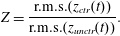(5.1) $$\begin{eqnarray}Z=\frac{\text{r.m.s.}(z_{ctr}(t))}{\text{r.m.s.}(z_{unctr}(t))}.\end{eqnarray}$$

In figure 6, it can be observed that the controller performance is gradually degraded when the amplitude rises and is saturated at approximately $\text{r.m.s.}(y)=0.6$ . The FXLMS compensator, instead, is able to maintain good performance until an abrupt breakdown of the performance around $\text{r.m.s.}(y)=0.6$ . At these large amplitudes, the compensator adaptivity cannot compensate the strong nonlinearities of the flow.

Variation of the free-stream conditions may also degrade the control performance, since it changes the baseflow. The wind-tunnel speed is varied around the design condition $U_{WT}=12~\text{m}~\text{s}^{-1}$ , changing the Reynolds number and, as a consequence, the stability properties of the flow (Schmid & Henningson Reference Schmid and Henningson2001). A white noise is low-pass filtered with a cutoff frequency of $4~\text{kHz}$ and considered as a disturbance signal $d(t)$ . The disturbance is monitored in order to ensure a 2D wavefront. The ratio between $\text{r.m.s.}(y)$ and the wind-tunnel speed $U_{WT}$ is kept constant and equal to $6.5\times 10^{-3}$ in order to avoid nonlinear effects. It should be noted that the asymptotic velocity $U_{\infty }$ differs from $U_{WT}$ because of blockage effects due to the presence of the flat plate and experimental equipment.

Figure 7(a) shows $Z$ as a function of the wind-tunnel speed variation ${\rm\Delta}U_{WT}$ . It is observed (blue dashed line) that the LQG performance is sensitive to variation of the free-stream velocity. One can note that the best performance is obtained for a velocity lower than the design speed. This shift can be attributed to the fact that an experimental flow can only be modelled numerically up to a certain accuracy. Uncertainties such as, for example, fluctuations in temperature (and thus a shift in Reynolds number) are unavoidable and lead to loss of performance, as described in the § 4. The FXLMS compensator, on the other hand, is able to adapt to the changed conditions. Even if the required input–output relation $u\rightarrow z$ – which is a static part of the FXLMS algorithm – is changed by the speed variation, the adaptive nature of the controller is able to compensate for this error and provide an almost unaltered performance for significant wind-tunnel speed variations.

Figure 7.

Effect of wind-tunnel speed variation ${\rm\Delta}U_{WT}$ on the performance indicator $Z$ . The solid line in (b) depicts the DNS data shifted to fit the experimental curve. The flow is excited by the disturbance source operated with a white-noise signal $d(t)$ .

The robust property of FXLMS is also confirmed by the numerical experiments (figure 7 a). Similarly to the experiment, the free-stream velocity is varied with respect to its nominal value and the performance of the control action is monitored. At the design conditions ${\rm\Delta}U_{WT}=0~\text{m}~\text{s}^{-1}$ , the model for which the LQG was designed is a very accurate representation of disturbance behaviour. Interestingly, the attenuation achieved by the FXLMS algorithm is very close to the optimal performance of the LQG regulator. For the latter compensator however, $Z$ increases linearly with ${\rm\Delta}U_{WT}$ . This can be explained as follows. Assume that $z(t)$ is the superposition of the two counter-phase TS waves, one generated by the disturbance source and one by the plasma actuator,

(5.2) $$\begin{eqnarray}z(t)=z_{d}(t)+z_{u}(t)=a\sin ({\it\omega}(t+{\rm\Delta}{\it\tau}))-a\sin ({\it\omega}t).\end{eqnarray}$$

The leading-order effect of a change in the free stream is on the phase speed of the TS wave, which in turn results in a modification of the phase-shift parameter ${\rm\Delta}{\it\tau}$ . On rewriting expression (5.2) to highlight the role of ${\rm\Delta}{\it\tau}$ ,

(5.3) $$\begin{eqnarray}z(t)=2a\sin \left({\it\omega}\frac{{\rm\Delta}{\it\tau}}{2}\right)\cos \left({\it\omega}\left(t-\frac{{\rm\Delta}{\it\tau}}{2}\right)\right)\approx a{\it\omega}{\rm\Delta}{\it\tau}\,\cos \left({\it\omega}\left(t-\frac{{\rm\Delta}{\it\tau}}{2}\right)\right),\end{eqnarray}$$

it is observed that for small values of ${\it\omega}{\rm\Delta}{\it\tau}$ , the amplitude of $z(t)$ is a linear function ${\rm\Delta}{\it\tau}$ . The black solid line in figure 7(a) shows the simulated LQG performance (dashed blue in figure 7 b) when it is shifted to the left to coincide with minima of experimental control values of $Z$ . It should be noted that $Z$ corresponding to numerical data asymptotically approaches the experimental data (blue dashed line), showing the same linear behaviour as predicted by (5.3).

Figure 8.

Compensator kernels $K(i)$ for different wind-tunnel speeds for LQG (a) and FXLMS (b). The solid line represents the design condition. When $U_{WT}$ decreases (dashed line) or increases (dotted line), the FXLMS compensator adapts to the new conditions by stretching or shrinking the compensator kernel.

The solid lines in figure 8 depict LQG and FXLMS kernels for the design condition, i.e. ${\rm\Delta}U_{WT}=0~\text{m}~\text{s}^{-1}$ . When the wind-tunnel speed is decreased, the amplification of the TS wave is reduced and the propagation speed of the TS wave decreases, i.e. the TS wave moves slower than under design conditions. In this particular new condition, the FXLMS algorithm reacts by stretching the convolution kernel in time and reducing the magnitude of the $K(i)$ coefficients (dashed line in figure 8 b). On the other hand, if the speed increases, the effect on the flow is opposite; the TS wave moves faster and is more amplified. Hence, the compensator reacts by shrinking the kernel and increasing the magnitude of the $K(i)$ coefficients (dotted line). The LQG kernel, instead, is fixed and does not adapt to the actual flow conditions.

Figure 9.

Correlation between the phase error $|{\rm\Delta}{\it\tau}|$ (squares) and the performance loss ${\rm\Delta}Z$ (dashed line) when the wind-tunnel speed is changed. The error bars report an interval $\pm {\rm\Delta}t$ around each ${\rm\Delta}{\it\tau}(U_{WT})$ point.

To quantify the phase shift in the kernel, let ${\it\tau}$ represent the time for which the kernel attains its minimum value. Further, one may define the difference between the phase shifts of the two compensator kernels by $|{\rm\Delta}{\it\tau}|=|{\it\tau}_{LQG}-{\it\tau}_{FXLMS}|$ . In figure 9, a strong correlation between $|{\rm\Delta}{\it\tau}|$ and the performance loss ${\rm\Delta}Z$ (i.e. the gap between the two curves in figure 7 a) is observed. This correlation shows that the compensator performance is depends mainly on a correct prediction of the time it takes for the TS wave to propagate from the reference sensor and to the plasma actuator. In the LQG approach, this information is given by the designed static model: any inaccuracy in this model may lead to an incorrect computation of the phase shift and, eventually, to a performance loss.

The FXLMS adaptive algorithm is not equivalent to a feedback sensor/actuator configuration (Belson et al. Reference Belson, Semeraro, Rowley and Henningson2013). The FXLMS algorithm is able to adapt to modified flow conditions (i.e. weak nonlinearities, free-stream variation, etc.) by adapting its response (e.g. by stretching/shrinking the kernel when velocity fluctuations occur). However, it has to be noted that (i) the measurement signal $z(t)$ does not have a direct influence on the control signal but only on the kernel and (ii) the adaptation time scale – approximately $15~\text{s}$ from zero initial condition to the asymptotic value – is significantly larger than the TS wave time scale. Therefore, the compensator is able to adapt only to slow changes in the flow, and the adaptation loop cannot be characterized as a conventional feedback. These results extend and confirm our earlier work on the Kuramoto–Sivashinsky equation to a physical fluid flow (Fabbiane et al. Reference Fabbiane, Semeraro, Bagheri and Henningson2014).