1. Introduction
Shifting cultivation is one of many phenomena involving the interaction of humans with their natural environment. Like many resource management issues, the spatial and temporal dimensions are essential to understanding the system. Fishermen expend varying levels of effort searching over spatially heterogeneous patches of ocean for their catch, itself a population that varies over space and time (Sanchirico and Wilen, Reference Sanchirico and Wilen1999). Forest resources cover vast areas, some of which are difficult (and therefore costly) to access. The timing and methods of cutting have a significant impact on extraction costs and long-term forest regeneration as well as the population dynamics of associated plant and animal species. In the Serengeti, wildlife migrates over vast distances to follow seasonal variations in rainfall and pasture. Pastoralists engage in similar movements over space and time. Even the classic von Thünen model (von Thünen, Reference von Thünen and Hall1826) of rural–urban land use and land values is based on the fact that land use varies over space and time.
Until recently, the tools of resource economists have focused primarily on one dimension of the resource allocation problem – optimal allocation of resource use over time. Economists have not, for the most part, addressed the spatial dimension (Sanchirico and Wilen, Reference Sanchirico and Wilen1999), treating the spatial dimension superficially at best and, with few exceptions, ignoring spatial dynamics (Bockstael, Reference Bockstael1996). However, ignoring the spatial dimension can lead to incorrect conclusions about the viability of alternative resource management strategies (Smith and Wilen, Reference Smith and Wilen2003).
Accounting for the spatial dimension makes it clear that land is not a costless factor of production, even when it is in abundant supply, due to the time required to travel between home and field (Stryker, Reference Stryker1976). While it is true that population growth and intensification of agricultural land use through shorter fallow cycles are closely linked (Boserup, Reference Boserup1965), there are other important factors, such as the degree of social cohesion in a village (Stryker, Reference Stryker1976), at play. Intensification (through shorter fallow periods) can occur even with abundant forest resources not too far away when village people either desire to work close to home or cannot relocate. Spatial relationships and individual preferences must be considered when modelling land use decisions and, by extension, intensification of land use and long-run resource productivity. Describing a dynamic spatial model of resource use by smallholder farmers, this paper addresses the limitations of previous decision-making models of resource use by incorporating both individual preferences over landscape characteristics and the spatial dimension of resource use. Use of a decision model based on stated preferences provides further insights into the nature and causes of land use intensification.
Household models and nonseparability
In shifting cultivation, the unit of analysis is a small household that relies almost entirely on its own labour resources to exploit the natural resources at its disposal in earning a livelihood. Although separable agricultural household decision-making models (Singh et al., Reference Singh, Squire and Strauss1986) are often employed in the developing world, in the context of subsistence agriculture, where some markets may be either incomplete, fragmented or missing, household consumption decisions are not often separable from agricultural production decisions. Production and consumption decisions occur simultaneously and, in many cases, the labour constraint binds. Non-separable household models (de Janvry et al., Reference de Janvry, Fafchamps and Sadoulet1991) better explain the dynamics of household decision-making in this context (Holden, Reference Holden1993a, Reference Holdenb; Holden et al., Reference Holden, Barrett and Hagos2003; Kuyvenhoven et al., Reference Kuyvenhoven, Ruben and Kruseman1998; Vosti and Witcover, Reference Vosti and Witcover1996), helping explain why subsistence households frequently appear not to respond to incentives as a profit-maximizing producer might. While a short-fallow system may appear to be optimal (Dvorak, Reference Dvorak1992) under certain restrictive assumptions, a nonseparable agricultural household model indicates that continued use of traditional shifting cultivation systems is often a rational economic choice (Holden, Reference Holden1993a, Reference Holdenb). Failure to account for important aspects of the decision-making context through inappropriate simplifying assumptions, such as separability, can lead to incorrect conclusions (Angelsen, Reference Angelsen1994, Reference Angelsen1999a, Reference Angelsenb).
Spatial resource modelling of shifting cultivation
Few spatial resource models have explored the spatial dimension of shifting cultivation beyond accounting for distance from markets (Omamo, Reference Omamo1998a, Reference Omamob) or the location of the agricultural frontier (Angelsen, Reference Angelsen1994, Reference Angelsen1999a, Reference Angelsenb). Deforestation models relying on satellite imagery are essentially data-driven empirical models and are often unable to disentangle the relative influence of loggers, commercial agriculture, and subsistence farmers (Mamingi et al., Reference Mamingi, Chomitz, Gray and Lambin1996). They fail to capture essential elements of a landscape dominated by the mosaic of small plots characteristic of subsistence agriculture at the forest frontier (Wilkie, Reference Wilkie1994). Their use for modelling the relationship between subsistence agriculture and environmental outcomes is limited because they do not describe the spatial process itself. Many economic models incorporating the spatial and temporal dimensions (Albers, Reference Albers1996; Albers and Goldbach, Reference Albers and Goldbach2000; Cropper et al., Reference Cropper, Puri and Griffiths2001; Geoghegan et al., Reference Geoghegan, Villar, Klepeis, Mendoza, Ogneva-Himmelberger, Chowdhury, Turner and Vance2001; Manson, Reference Manson2000; Pendleton and Howe, Reference Pendleton and Howe2002; Pfaff, Reference Pfaff1999; Thornton and Jones, Reference Thornton and Jones1998; Turner II et al., Reference Turner II, Villar and Foster2001) rely on overly simplistic models of the household, implicitly assuming separability of production and consumption decisions.
Shifting cultivation, as a spatiotemporal phenomenon, differs significantly from other forms of subsistence agriculture. New patches of land are selected and cleared annually or semi-annually. Forest resources provide patches of land for agricultural production as well as non-wood forest products harvested from that same mosaic of forest and agricultural land. In its ‘purest’ form, the area of active cultivation literally shifts across the landscape. In other circumstances, where households or extended families retain rights of access and use to land over a period of years, the pattern is different – the area of active cultivation for each household cycles through a defined set of land holdings. In either case, temporary forest clearing permits one to three years cultivation followed by extended periods of forested fallow. A dynamic mosaic of forest, fallow, and cultivated land at the forest margin is the result. Assessment of the long-term sustainability of farming systems and the ecological integrity of the forest landscape requires an understanding of the dynamics of this mosaic of land use.
This paper makes three main contributions to the modelling literature. I develop a theoretical conceptualization of the spatiotemporal problem that does justice to both the decision-making context found in developing-country agriculture and the spatiotemporal dynamics of resource use. The model extends the essential elements of a nonseparable household model to incorporate a dynamic model of spatial resource exploitation, thereby addressing the limitations of current household and bio-economic resource models. This modelling approach has broader application to modelling spatio-temporal phenomena in general, including other forms of subsistence agriculture, forest resource management, and pastoralist systems. Secondly, I develop an empirical specification of the decision rule that functions in data-sparse environments and responds to household-specific preferences over landscape characteristics. Finally, I integrate the empirical decision model into a structural simulation model of shifting cultivation and demonstrate it using a group of households in a southern Cameroon village. Although based on a limited data set, it serves as a proof-of-concept and gives insight into alternate explanations for the shortening of fallows in shifting cultivation systems.
2. A spatiotemporal household model of resource use
The forest resource
In the context of shifting cultivation, agricultural productivity depends primarily on the stock of soil fertility or nutrients, N, available at time t. Unlike Sanchirico and Wilen's (Reference Sanchirico and Wilen1999) model of renewable resource exploitation, there is no dispersal between patches.Footnote 1 Forest (re)growth is modelled as nutrient accumulation over time for a patch of forest or fallow, s Footnote 2

where g(N st) is the nutrient growth function and g N ≥ 0,g N N ≤ 0, g ≤ ḡ.Footnote 3
It is also essential to account for use or extraction of nutrients by agricultural production. When the patch is in fallow, forest-fallow, or forest, there is growth of the biomass or nutrient stock (the function g(.) above).Footnote 4 Conversely, during clearing and subsequent cultivation, the nutrient stock ceases to accumulate and depletion occurs. There are two major sources of nutrient loss or use. Burning, b(N), the principal means of land preparation, amounts to a significant loss of biomass and the nutrients it contains, although it also makes a considerable amount available as ash for more or less immediate uptake by crops. Subsequent cultivation, c(N), further depletes the remaining nutrient stock, the rate of decrease depending upon the stock available for use.Footnote 5 Assuming that forest regrowth does not occur at the same time as cultivation (extraction), the model for nutrient accumulation and extraction over time for a particular patch of forest, s, is

where

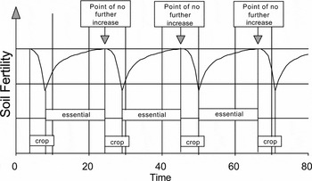
When u st = 0 and u st−1 = 0 (i.e., when the patch is in fallow), only the forest growth function, g(N st), is operable. When u st = 1 and u st−1 = 0 (i.e., the plot was in forest in the previous period, but is now cleared for cultivation), the nutrient use/loss functions for burning and cultivation, b(N st) and c(N st), are operable. Finally, when both u st = 1 and u st−1 = 1 (i.e., the plot was cultivated in the previous period as well as the current period), only the nutrient use function for cultivation, c(N st), is operable. The result, for any land patch, is the characteristic pattern of soil fertility associated with optimal household decisions in shifting cultivation systems and illustrated in Figure 1.Footnote 6 The period marked ‘essential’ indicates the length of fallow required for soil fertility to recover to its maximum. Should the fallow period shorten, the average fertility will decline over time. In order to ensure a steady supply of food to meet subsistence and cash income requirements, a household requires several patches at various stages of cultivation and regeneration (fallow) at any point in time.
Nutrient dynamics typical of shifting cultivation where there are alternate cycles of cultivation and forest regrowth (after Hauser et al., Reference Hauser, Nolte and Salako2001)

The household
I assume that a household, i, in a community has a stock of land, Ω, at its disposition, where  . That stock of land is made up of a finite (
 ), but potentially variable, number of patches or plots of land, s, that are in various stages of development along a continuum from mature forest, to forest-fallow, young fallow, and active agricultural fields as represented by the fertility level N. The household decision-maker's task is to allocate available labour resources for agricultural work to their most efficient use across the available patches of land, while ensuring subsistence needs are met and the labour stock of the household is maintained in the long term.Footnote 7
Because the principal emphasis of subsistence agricultural households is on food production for home consumption, the resource exploitation model developed here focuses on the mixed food crop field, which, in the Congo Basin of Cameroon at least, is the primary food source for the subsistence household.Footnote 8 Sale of any surplus production provides cash for other household needs.Footnote 9 The household's objective is to maximize the discounted utility, U, derived from food surplus, q tf (for consumption and sale over and above a subsistence constraint), and leisure, l t (actually non-labour activities, i.e. activities not associated with agricultural work)Footnote 10 in each period t
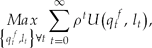
where  is the discount factor and δ is the discount rate.
Since labour requirements for clearing and burning of fallow, forest fallow, and forest generally increase with the age of the stand (whether measured in terms of chronological age, biomass, or nutrient stock), it is possible to model labour requirements for clearing as a function of N. The rate of increase is not constant, but assumed to decline as fertility, and therefore age, of the fallow or forest stand increases. Following Dvorak (Reference Dvorak1992), the relationship is

On the other hand, labour requirements for cultivation (weeding in particular) vary inversely with the age and, by extension, the fertility of the fallow or forest stand cleared for cultivation. One of the major limitations to long-term cultivation of forest plots, in addition to declining fertility, is the cost of weed control. Fallow periods are as much to control weeds as to restore fertility. After a short fallow, the large stock of weed seeds germinate when the land is cleared. However, with a longer fallow period, many of the annual weeds will have died out. When such a forest-fallow plot is cleared, the labour cost of weed control will be significantly reduced. Since higher soil nutrient status and fallow age are directly related, we can combine the two and say that labour for weeding and the nutrient status of the fallow are inversely related. Therefore, labour requirements for weeding are effectively a function of nutrient status, N Footnote 11

Labour requirements for travel to and from a particular patch of land are also an important factor in labour use. The total labour required for fieldwork is adjusted by a travel time factor based on the distance, d, from the village to the particular patch, as well as the proximity to other fields, f, or patches being actively cultivated. The travel time adjustment factor is

where k ∈ [1, ),k d ≥ 0,k f ≥ 0 and is the maximum feasible time to walk to do a day's work.
The labour constraint is as follows

Substituting the labour requirements into the labour constraint gives

which can be solved for l and substituted into the utility function.
The evolution of the stock of available labour depends on three factors.Footnote 12 The rate of natural change of the household labour force, γ, captures the impact of births, deaths, and aging on the household. It is the net change in working-age population on a year-to-year basis. The general state of health and well-being of the household members influences the amount of time available for work and leisure, η; fewer labour resources are available as health or general well-being decline. Increases in household size, m, arise through marriage or in-migration.Footnote 13 I assume γ, η, and m to be exogenous to the model itself.Footnote 14 The labour stock law of motion is
![\begin{eqnarray}
\Delta L_t^T = L_{t + 1}^T - L_t^T = \gamma L_t^T - \eta L_t^T + m_t,\,{\rm where}\,\,\gamma \in \left({- 1,1} \right)\,{\rm and}\,\eta \in \left({0,1} \right].
\end{eqnarray}](https://static.cambridge.org/binary/version/id/urn:cambridge.org:id:binary:20160115084306094-0212:S1355770X08004415_eqn9.gif?pub-status=live)
Food production (yield) on a particular patch of land depends on the level of nutrients in the soil at the time of cultivation. While also influenced by the amount of labour input, for the purposes of land-clearing decisions it is assumed that households have an intuitive knowledgeFootnote 15 of the optimal labour allocation associated with different levels of soil fertility as represented by fallow or forest types and ages.Footnote 16 As a result, the patch-level production function is

Therefore, the food surplus over-and-above the subsistence constraint is
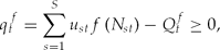
where Q tf = aL tT is the subsistence requirement and a is the per capita consumption of food, assuming per capita food demand to be perfectly inelastic.
The household's problem and the first-order necessary conditionsFootnote 17
After substituting the subsistence and labour constraints into the objective function, the complete nonseparable model for a subsistence household is therefore
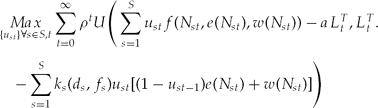
subject to

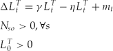
To summarize, the subsistence household maximizes the sum of the discounted utility derived from food consumption and leisure subject to law of motion constraints on patch-specific nutrient stocks and on household labour supply when deciding the location of food crop production among the patches of land available to the household (i.e. the choice set S).
This constrained dynamic optimization problem can be solved using the Maximum Principle. Assuming that the choice variable u st is continuous on the interval [0, 1] and represents the proportion of the patch being cultivated, the first-order conditions (FOCs) can be derived from the Hamiltonian, simplified and rewritten to facilitate interpretation (after Conrad, Reference Conrad1999).
The maximal condition simplifies to

The co-state equations simplify to
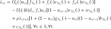

The laws of motion take the form


Typically, one derives the steady state by evaluating the first-order necessary conditions when the control and state variables and the multipliers λ and ϕ are unchanging. Eliminating the time subscripts from u, N, L, λ, and ϕ, the co-state equation (23) and law of motion (25) involving labour become


However, due to the nature of shifting cultivation, which is more like a ‘pulse’ fishery (where the stock is harvested very intensively at an unsustainable level for a short period of time and then left to recover on its own) or the periodic clear cutting of a stand of forest, eliminating the time subscripts from the maximal condition (21), the co-state equation for N (22), and the nutrient stock law of motion (24) is not advisable. Although there may be a steady state for household labour resources, the very nature of resource extraction in this context means that there is not a steady-state level of soil nutrients and crop harvest on an individual patch of land, although there should be a long-term average level of the nutrient stock (see Figure 1).Footnote 18
While it is conceivable that one could solve for the dynamic equilibrium, it is not practicable due to problems with tractability.Footnote 19 Deriving the first-order conditions required an implicit assumption that the indicator variable u st is continuous, in essence indicating the proportion of a particular patch of land that would be cultivated in a particular year. This would work well should a patch be defined to be a reasonably large plot of land, at a scale where one would not clear the entire area in any one year. However, to facilitate explicit modelling of the spatial dynamics, it is important to choose a relatively small patch size. By doing so, any one patch would either be cultivated or not in any one year, with the farmer choosing the most preferable patches to cultivate in their entirety and leaving the rest for future years. When a patch is not cultivated (u st = 0), the maximal condition (before rearranging) is strictly less than 0. Conversely, when a patch is cultivated in its entirety (u st = 1), the maximal condition is strictly greater than 0. As a result, patches can be sorted and compared according to the sign and value of the maximal condition. The decision-maker, therefore, chooses among available patches based on that which is most preferable at a point in time, according to his or her own criteria.
Using the simplified form of the maximal condition (21), the basis for this comparison is
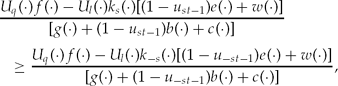
where s and −s refer to any two patches and where −s ∈ S such that −s ≠ s. The patch with the greatest marginal net benefit when put into use should be chosen over all of the others in any particular year. The total number of patches cleared in any one year depends upon the labour resources available to the household. Equation (28) generates a preference ordering of patches at each time period, implicitly accounting for time preferences. As will become clear in the discussion of the empirical model, individual decision-makers have preferences over time-varying characteristics of patches of land that, in effect, incorporate their discount rate into the decision-making process. Given such a preference ordering, it is possible to derive the relative suitability of individual patches of land from the point of view of the household. Clearly, the relative attractiveness of any one patch at a point in time will depend on a number of factors:
• the relative value attached to food in comparison to leisure time because of differences in labour requirements by patch;
• declining productivity of a patch over time as compared to the labour saved by not moving to a new patch and clearing it for cultivation;
• different rates of nutrient accumulation for patches of different fallow age.
3. Empirical model of decision-making
The attractiveness or suitability of any particular patch of land depends not only on the characteristics of the patch itself (relative to other patches available to the household) but on personal preferences with respect to these patch-specific characteristics. Since a household chooses to cultivate the patches s, giving the greatest marginal net benefit or utility at a point in time as shown in equation (28), the reduced form of the decision criteria for household i is

where u st* is a measure of the overall suitability of patch s in time t, a latent variable; Zst is a vector of plot-specific factors or characteristics, some of which may change endogenously over time; Xit is a vector of household-specific factors that may change endogenously over time; and Wit is a vector of exogenous socio-economic variables specific to the economy, the village, or the household.Footnote 20
The vector Zst includes factors such as the age of the fallow at clearing, fertility status, N, length of time under cultivation, proximity to the village, d, proximity to other currently cultivated fields, f. It also includes variables such as the presence of indicator species for soil fertility and proximity to neighbours' fields, which serves as a proxy for the risk of encroachment by neighbours and the potential for reducing the size of the choice set in future periods.Footnote 21 The others provide additional information about the fertility status of a patch of land. The vector Xit includes the stock of available labour, L, at time t; in or out-migration of labour resources, m; the size of the household's land holdings, S; availability of additional forested land within the clan or village and other household-specific demographic or socio-economic variables. Finally, the vector Wit includes the per capita subsistence food requirement, a; the rate of natural change of the household labour force, γ; the impact of the general state of health and well-being of the household members on the amount of time available for work and leisure, η; the period for which a household retains land use rights to fallow patches (s ∈ {Ω}u st = 0) of land within their stock of land, Ω; and the set of characteristics associated with the village location such as market access, costs of transport, and the relative prices of market goods.
Changes in factors (m > 0, γ) which directly or indirectly increase the stock of labour, L, will have an effect on both the total number of patches cultivated in any year and indirectly on the utility derived from cultivation. This occurs either through increased leisure, with more time left over after doing the same amount of work, or through a larger food surplus, q, above subsistence needs, Q, as food production increases without sacrificing leisure. The reverse will be true for factors (m < 0, η) that directly or indirectly decrease the stock of labour, L. Migration, m, is a function of agricultural prices, prevailing urban wage rates and employment opportunities as well as movements related to marriage of household members. Each of these influence livelihood choice and have a direct impact on the amount of labour devoted to subsistence agriculture.
The location of a patch of land relative to the village, d, and relative to other patches under cultivation, f, has a direct impact on its perceived suitability for cultivation. Other things being equal, a patch that is farther from the village is less attractive due to the increased cost of travel to and from home each day. Similarly, patches located in close proximity to others currently in cultivation mean reduced travel costs since it is possible to combine trips to multiple patches. This is particularly true for patches in which, for example, previously planted cassava and plantain is harvested gradually as household needs dictate. Fields located closer to these are more attractive as they do not require a special trip to harvest them when they mature.
The size, , of the discrete choice set, Ω, among which a household can choose patches for cultivation at any one time, will also influence the returns to cultivation. With a larger choice set, for example, a household can leave land in forest-fallow longer and thereby benefit from improved fertility (higher yields) and reduced weeding labour requirements.Footnote 22 The dynamics of the choice set depend on particular customs related to land tenure and effective use of the land by the household. Depending on these customs, some patches may be lost to the household if they are not cultivated often enough while, on the other hand, the choice set could expand if there is additional forest belonging to the clan or village that the household could clear and claim.Footnote 23
Production technology may affect the relative costs of labour devoted to land clearing, b(N), as compared to the labour cost of cultivation (especially weeding), c(N), and therefore the relative suitability of different patches of forest or fallow land. Since costs of land clearing increase with N or biomass and, therefore, with the age of the fallow, anything that reduces the cost of clearing older biomass relative to younger fallows (e.g., a chain saw) will make older fallows relatively more attractive since labour costs associated with cultivation, and weeding in particular, decline as N increases. The reverse will apply for technological changes that reduce the labour cost of weeding younger fallows relative to the cost of older ones since c(N) is decreasing in N or biomass and, therefore, fallow age. Similarly, the way in which household decision-makers assess the relative importance of time spent in either land clearing or cultivation will change the relative suitability of different patches.
Decision criteria and estimation results
Ultimately, what matters for the pattern of land use over space and time is the relative attractiveness of individual patches of land from the decision-maker's point of view. It is therefore important to understand the decision criteria households use when deciding where to cultivate each year among available forest or fallow lands. Each cropping season, farmers make a series of decisions with respect to where to cultivate, how much land to clear, and the particular mixture of crops to plant. Their actual decisions depend upon criteria that include not only the physical characteristics of the natural resources at their disposal (forest, forest-fallow, and fallow land patches) but on personal preferences and household-specific demographic characteristics. The result is the particular mosaic of land use observed today and its evolution over time.
Although estimation of a reduced-form model using revealed preferences to determine the likelihood of clearing a patch as a function of household attributes and specific characteristics of the landscape is the most common approach, it requires attribute information about all available patches of land (used and unused, cultivated and fallow). Not only is this approach infeasible in the circumstances, given the data required, it ignores considerable information about the nature of the preferences that underlie the observed behaviour.
Alternatively, one can use stated preferences. The argument against this approach is that stated preferences may not correspond to actual or revealed behaviour – stated and revealed preferences may diverge (Brown, Reference Brown2006). In fact, this is to be expected when individuals make decisions. They have preferences over different attributes of a resource (for example, soil fertility and the distance of a field from the village) and trade-offs have to be made between these characteristics. Additionally, there may be binding constraints on labour resources that limit the distance one can travel to do work or different spatial patterns of resource availability or access. Some household decision-makers may face very definite soil fertility–travel time trade-offs.Footnote 24
Use of stated preferences permits considerable insight into the decision-making process and outcomes. Since it is possible to ask decision-makers directly about the importance they place on different attributes, and it is generally much cheaper and easier to survey households rather than every plot in a vast landscape, in the empirical implementation I use survey-based rather than regression-based weights on the vector of patch characteristics.Footnote 25
Equation (29), the reduced form of the decision criteria, can be rewritten so that the overall suitability of each patch available to a household can be thought of as

Each patch of land has observable characteristics, the vector Zst, which can be objectively measured and compared to other patches using GIS (Geographic Information Systems) techniques. These observable characteristics include the age of forest or fallow regrowth, the fertility of the soil (measured by the presence of indicator species), the travel time or distance to the village, the proximity to other cultivated fields, etc.Footnote 26
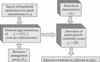
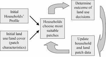
At the same time, each household attaches differing levels of importance to these characteristics, represented by the time-varying preference parameter vector rit, which is itself a function of household-specific characteristics, Xit.Footnote 27 As a result, stated preferences may vary over time according to changes in household-specific characteristics. The elements of  it can be estimated individually using a series of ordered logit models relating the importance of a particular patch characteristic r it in the vector rit to the household-specific Xits (see Appendix 1 and Brown (Reference Brown2004, Reference Brown2006) for details of variable selection and data collection). The value for u st* is then determined based on it and the plot-specific characteristics Zst at the beginning of period t. I assume that a household will choose to cultivate those patches with the highest scores according to what is feasible given available labour resources, L. Figure 2 illustrates the decision rule estimation and implementation sequence. Individual patches are compared as in equation (28), thereby embodying both household-specific preferences implied by the analytical model as well as landscape characteristics. Equation (30) serves as the key decision-making function and, when combined with the laws of motion for household-level labour resources and patch-level soil fertility as well as the constraints on labour and food production in the structural simulation model, enables simulation of the evolution of land use over space and time (Figure 3).
Schematic diagram of decision rule estimation and implementation

Dynamics of the spatiotemporal simulation model

A household survey conducted in three communities in southern Cameroon during the spring of 2003 (Brown, Reference Brown2004, Reference Brown2006) quantified individuals' assessments of the relative importance of the various factors influencing their decisions (the vector rit). It considered decisions about field location and size as well as decision-makers' assessments of the suitability for cultivation of different aged patches of fallow and forest for the main agricultural field types, including the mixed food crop field cultivated for subsistence food crop production. The factors evaluated in terms of their importance in decision-making included not only those normally considered to be of economic importance, i.e. fallow age (and, therefore, soil fertility) and distance from the field to the village, they also included the importance of non-traditional factors including the proximity of the patch to the area currently being cultivated, the presence of an invasive weed species, the strategic choice of location in order to protect long-term land use rights to one's land holdings, and whether or not the patch could be cleared and still leave adequate time for drying down in advance of burning. Most of the responses to each part were solicited using a modified form of an indigenous board game (Franzel, Reference Franzel, Peters and Pingali2001) common in the area.Footnote 28 Linking it to household-level socio-economic and demographic data from a resource management survey of the same households conducted previously by the International Institute of Tropical Agriculture (IITA, 1996) permitted estimation of the relationship between rit and Xit. Appendix 1 reports the results of ordered logit estimations of the importance of five of the decision criteria used when deciding where to clear land for a mixed food crop field. The data set, while small, is sufficient to demonstrate the usefulness of the modelling approach.
4. Spatiotemporal simulation of land use decisions
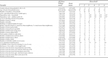
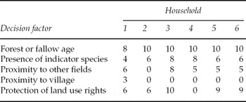
Having estimated stated preferences as a function of household-specific characteristics, we can determine the relative suitability for subsistence food crop production of the different patches of forest that are available to a household. That is, we can derive u st* as a function of the estimated preference parameter vectorit and plot-specific characteristics Zst for a specific set of household characteristics Xit as in equation (30). Ranking of the relative suitability of patches of forest and fallow land is household- and period-specific; differing across households and within households over time. One can, therefore, characterize different household types within each of the communities and model their land use choices over space and time. Tables 1 and 2 summarize the household characteristics and predicted scores for the five main decision criteria for six such households in one of the Cameroon survey communities.
Socio-economic profile of the six households used in the simulation model demonstration as compared to the village and sample means

Notes: Standard deviations are in parentheses.
* ‘out of 10’ – respondents scored the contribution of the four income sources to total income by allocating ten seeds among the four income categories.
Predicted importance scores for six households at the start of the simulation

The six households included in the simulation model represent the range of characteristics found in the data for the village of Awae – including the age, gender, and educational level of the household head, the household size and dependency ratio, the household's land holdings and the importance of farm and non-farm sources of income. The importance placed on different characteristics varies considerably. While nearly all households place a very high level of importance on soil fertility as represented by fallow age and a relatively high importance on soil fertility as measured by indicator species, only household one is concerned about the proximity of their fields to the village. Conversely, all but household two place considerable importance on clearing new fields in close proximity to those already in production to minimize travel time between fields, reflecting the fact that second-year agricultural plots contain cassava and other crops harvested periodically after annual crop cultivation ceases. Finally, unlike the others, household four places no importance on protection of long-term land use rights in the choice of location to clear for cultivation. This household is relatively land rich (see Table 1) in terms of relative land holdings and in the number of plots of land in fallow – especially when compared to the area actually in cultivation. Conversely, household four earns a relatively large proportion of its income from non-farm sources.
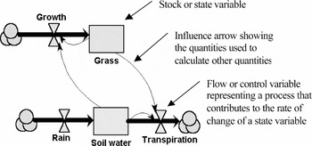
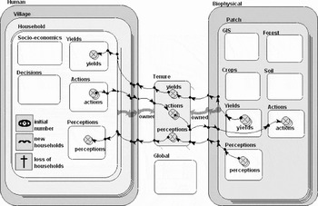
I used the Simile modelling environment (Muetzelfeldt and Massheder, Reference Muetzelfeldt and Massheder2003) to develop a structural spatiotemporal model of several households and the associated village landscape (Brown, Reference Brown2004, Reference Brown2006; Legg and Brown, Reference Legg and Brown2003). Simile facilitates modelling interactions between humans and their environment (Muetzelfeldt and Massheder, Reference Muetzelfeldt and Massheder2003) with stocks evolving dynamically as they respond to changing flows of resources using difference equations that change the state variables (Figure 4). Stocks may refer to decisions or priorities as well as to physical elements on the landscape. Flows may refer to changes in priorities or decisions as well as to physical factors that increase or decrease stocks over time. Simile supports individual-based modelling of, for example, households or patches of land (Legg and Brown, Reference Legg and Brown2003), facilitating construction of multiple instances of model components. Definition of conditional and dynamic relationships between various model components (Figure 5) permits simulation of growth and production of food crops on various patches of land, regrowth of forest during fallow periods (equation (13)), and transfer of outputs to the appropriate household. On the household side, labour and subsistence constraints (equations (8), (9), and (11)) are explicitly modelled for each household since allocation of labour resources has an impact on crop production. Parameters for yield response, and labour and consumptions norms are drawn from prior research and modelling work in the study area (Gockowski and Nolte, Reference Gockowski and Nolte2003; Leplaideur et al., Reference Leplaideur, Longuepierre and Waguela1981).
Diagrammatic representation of stocks and flows in Simile

Layout of a simulation model in Simile

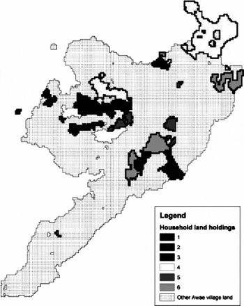
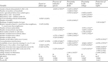
The model's decision-making component explicitly uses the decision rule specified in equation (30) and the sequence of events illustrated in figures 2 and 3. The estimated regression parameters (table A1) and the initial socio-economic profile of the households (elements of the vector Xit from Table 1) together with a base map of the village (Figure 6) initialize the model. Within the model, the preference parameters ( it from Table 2) are updated at each time step and combined with measures of the physical landscape parameters (Zst) to derive the score (u st*) for each patch of land in a household's land holdings and guide the choice of patches for cultivation from season to season. The vector of exogenous socio-economic parameters Wit is assumed constant during the course of a simulation. The score for each patch available to a household dynamically evolves in response to changes in household preferences and the physical landscape as the patches of land change from agricultural land to fallow and then to forest. The elements of the preference parameter vector incorporate the household's valuation of the important attributes of the landscape. Time preferences (and, by extension, the discount rate) are implicitly incorporated through the importance placed on fallow age and indicators of soil fertility, both of which vary directly with fallow duration. Farmers who place less importance on fallow age, for example, are more likely to clear younger fallows – an indication of the shorter time horizon associated with higher discount rates. The number of patches cleared each season is a function of soil fertility and household consumption requirements provided that the labour constraint is itself not binding. As mentioned above, Figure 3 illustrates the dynamics of the simulation model.
The rasterized base map of Awae village showing the land holdings of the six households included in the simulation model

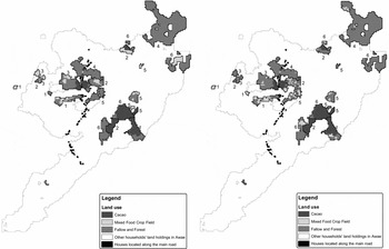
Figure 7a shows the initial location of mixed food crop production for each of the six modelled households. Over the course of a 20-year simulation, the zone of active cultivation (the location of the mixed food crop field) gradually shifts across a household's land holdings to that shown in Figure 7b. In fact, every rainy season each household clears one or more patches of land for active cultivation and abandons a similar number of patches to fallow. Any individual patch is cultivated for a period of only three years in a row. It is then abandoned to fallow – allowing the forest to re-grow for five to 25 or more years during the extended fallow period. Therefore, every year during each of the two rainy seasons one or more patches change land use from fallow to active cultivation and a similar number return to fallow. While it is not possible to see it clearly in the figures shown here, the pattern of land use varies among the households. Households two and five, for example, maintain a dispersed pattern of land use across their entire land holdings. Conversely, households one and six appear to cycle more intensively through a subset of their holdings, in some cases reusing the same patch of land for cultivation more than once during the course of the simulation. This is not only due to differences in their initial land holdings, but also due to their specific preferences over patch characteristics.
Initial (left map – 7a) and final (right map – 7b) land use for the six households for a 20-year simulation

The six households exhibit the range of spatial patterns of land use over time that can be observed in the field – some cultivating very close to home with very short fallows, others cultivating over a range of distances but with longer fallows, and others with isolated fields dispersed across the household's land holdings in a mosaic. These various patterns were found in aerial and satellite imagery and GPS base mapping exercises conducted as part of the Alternatives to Slash and Burn (ASB) research project in Cameroon (Gockowski et al., Reference Gockowski, Tonye, Baker, Weise, Ndoumbé, Tiki-Manga and Fouaguégué2004; Legg, Reference Legg2002, Reference Legg2003; Legg and Robiglio, Reference Legg and Robiglio2001a, Reference Legg and Robigliob).
Simulation results show differences in land use intensity as measured by fallow length, in crop productivity due to soil fertility, and the size of the surplus over-and-above subsistence requirements (Brown, Reference Brown2004, Reference Brown2006), even after controlling for household size and labour resources. These arise not only due to differences in population density but due to differences in individual preferences and in landscape-level initial conditions. As stated preferences over different landscape characteristics interact with each other, labour constraints, and the spatial distribution of land holdings, different patterns of land use and forest succession emerge. These patterns indicate preference-dependent and path-dependent intensification. Some households cultivate a subset of their land holdings more intensively (more frequently, meaning shorter fallows) because they prefer to be closer to their village or to other fields even though this may mean poorer agricultural productivity in some cases. The impact depends not only on preferences, but also on the individual pattern of land holdings. Spatial path-dependence arises because some households have more of their land holdings closer to the village, while others are either located further away or more dispersed in the forested area around the village. This helps explain some of the variation in fallow length observed in the village of Awae, where the size of land holdings is not limiting for most households (Brown, Reference Brown2006). Revealed preferences over fallow age, for example, diverge from stated preferences leading to shorter fallows than some households consider preferable. Through explicit modelling of the interaction between stated preferences and associated constraints, it becomes possible to identify two sources of intensification in addition to increasing population density.
5. Discussion and conclusion
This paper has discussed essential issues related to modelling of forest clearing and cultivation decisions in space and time. Incorporating the spatial dimension into dynamic resource use decisions makes possible modelling their landscape-level impacts over time. Additionally, I have discussed essential elements of human decision-making models where consumption and production decisions are non-separable, a crucial feature for dynamic models in the context of subsistence agricultural production. Simplifying assumptions that neglect these considerations for the sake of analytical tractability unfortunately risk failing to capture elements essential to understanding human behaviour when subsistence farming households make spatiotemporal resource use decisions, as at the forest margins in central Africa, for example.
The analytical model of subsistence agricultural production is both spatially explicit and dynamic. While impossible to solve analytically due to issues of tractability, the model incorporates the essential elements of decision-making and the key household-level factors that might influence the spatial location of agricultural production. This analytical model motivates a structural simulation model driven by a decision rule based on an estimable reduced-form model. In essence, it uses stated preferences for different characteristics of the resource (forest and fallow land for subsistence food production) and links them to household-specific characteristics, some of which themselves vary over time. The resulting time-varying preference parameter vector, when multiplied by a vector of plot-specific characteristics, assigns a suitability score to each of the plots of land available to a household. This plot-specific suitability score embodies the essential elements of the maximal condition of the analytical model. The household then chooses to cultivate those plots that are most suitable in any one year within the constraints of labour availability, subsistence food needs, and spatial distribution of land holdings, resulting in a revealed pattern of behaviour exhibiting the range of patterns of land use found in the area.
Having incorporated this decision-making model into a structural simulation model of subsistence agricultural production (Brown, Reference Brown2004), it is demonstrated here using a limited data set. Given the significant heterogeneity of household characteristics and the fact that decision-makers are influenced by their neighbours' choices, the model simulates several households simultaneously. By proceeding in this fashion, it is possible to simulate the differential impact of changes in exogenous parameters on household decisions (and hence the pattern of land use) as well as how land use patterns change over time as household-specific characteristics change.
One of the most helpful insights arises from the use of stated preferences over fallow length and other landscape characteristics. Revealed preferences for fallow length diverge significantly from those stated by some households. To understand the reasons for shortened fallows (intensification of production), it is important to get beyond revealed behaviour to the interplay between individual preferences, household resources and constraints. In some cases, short fallows arise due to lack of land resources. This is the standard Boserupian hypothesis for land use intensification (Boserup, Reference Boserup1965). However, as this simulation model shows, some simply prefer short fallows. Others shorten fallows due to a strong preference to cultivate close to home or to other existing fields – a preference that outweighs their stated preference for older fallows – even when abundant fertile forests or fallows are available. Finally, others have no strong preference to cultivate close to home, but wind up with short fallows all the same since, due to the spatial distribution of their land holdings, they lack more suitable land close at hand.
An appropriate policy response designed to promote sustainable livelihoods and ecosystems in the face of shortening fallow periods depends on the reason for intensification. Simply improving access to land will not result in longer fallows if, for example, they are short because households have a strong preference for short fallows or cultivation close to home. Shifting cultivation is a sustainable long-term strategy provided not only that there are sufficient land resources to maintain long fallows, it is also important that individual decision-making criteria be such that people choose to maintain the long fallows that are essential to the regeneration and maintenance of soil fertility.
This paper describes the development and initial testing of a theory-based spatially explicit decision-making simulation model and demonstrates its use on a limited data set. It successfully generates the dispersed pattern and variations of intensity common in shifting cultivation. Subsequent detailed validation will require an enhanced household data set and spatially explicit longitudinal data on land use. Further development of the simulation model will enable modelling either individual households or a collection of representative households at the village scale in order to effectively describe the spatial mosaic of forest resource use that evolves over time. Ultimately, this work should serve to develop an effective tool for analysis of the sustainability of subsistence agricultural practices at the household level, in terms of livelihood, as well as at the landscape-scale, in terms of land cover change and biodiversity conservation.
Appendix 1 – Ordered logit estimation results
Table A1 summarizes the ordered logit estimation results for five of the decision criteria – those of most importance to household decision-makers and which lend themselves to direct incorporation in the simulation model. Survey respondents scored the importance of each decision criterion independently on a 0–10 scale. The estimation strategy was to obtain the best possible prediction of the score for a specific criterion rather than to investigate the specific effect of a set of regressors on the importance score. For this reason, and given the small size of the data set, I initially used a stepwise OLS procedure to select the variables for inclusion in the subsequent ordered logit estimation.Footnote 29 Unlike the normal distribution, which underlies the ordered probit, the logistic distribution has a closed-form solution and the estimated parameters can be used directly in the simulation model to update the predicted scores during the course of a simulation. Given the nature of the estimation strategy, care needs to be taken in interpreting the specific regression coefficients. The goal was to find the best predictors of the score for a specific decision criterion and not an estimate of the precise contribution of any one independent variable to the score itself.
Ordered logit estimation results for the importance of five decision criteria

Standard errors are in parentheses.
*** indicates coefficients are significant at 1%, ** at 5% and * at 10%.