


1 Introduction
In oceanic and atmospheric flows, mesoscale eddies – which can alternatively be interpreted as Rossby waves – drive the convergence of momentum and potential vorticity (PV) fluxes, which in turn force and alter the large-scale flow and stratification. In the present study, Rossby waves in uniform background flow are excited in the linear shallow-water model by a localised, oscillatory forcing, referred to as a plunger and intended as a simple representation of transient eddy forcing. Such a forcing is also motivated by the growing awareness that eastward jets such as the Gulf Stream or Kuroshio are maintained by transient eddy flux divergences (Shevchenko & Berloff Reference Shevchenko and Berloff2016). The nonlinear zonal momentum flux convergence, estimated from the self-interaction of the linear Rossby wave response, is the primary concern of the study, with analysis of the role played by the uniform zonal background flow.
A number of previous studies have analysed the excitation of Rossby waves and the corresponding nonlinear mean-flow generation. In Haidvogel & Rhines (Reference Haidvogel and Rhines1983) nonlinear simulations of the plunger-forced quasi-geostrophic (QG) system exhibit (eastward) zonal momentum flux convergence at the forced latitudes, with adjacent westward recirculation zones. This pattern of zonal momentum flux convergence is equivalent to northward (poleward) convergence of PV fluxes. The corresponding theory was discussed by Thompson (Reference Thompson1971) – as Rossby waves propagate meridionally away from the forced location, they drive zonal momentum fluxes in the opposite direction, resulting in a time-mean convergence of zonal momentum fluxes at the forced latitudes. Waterman & Jayne (Reference Waterman and Jayne2012) built upon the study of Haidvogel & Rhines (Reference Haidvogel and Rhines1983) by considering in more detail the behaviour of momentum and PV fluxes, and by more deeply exploring the parameter regime. In addition, Waterman & Jayne (Reference Waterman and Jayne2012) constructed Green’s function solutions to the linear system, and showed that the nonlinear self-interaction of this linear response is qualitatively similar to the fully nonlinear case. This important result was also attained in Berloff (Reference Berloff2015) in which the analysis is extended to the multi-layer QG system with a uniform background flow. Furthermore, Berloff (Reference Berloff2015) demonstrated the applicability of the linear plunger-induced dynamics by implementing a parameterisation of mesoscale eddies based on the time-mean PV flux convergence and its dependence on the background flow. Berloff (Reference Berloff2016) followed on from Berloff (Reference Berloff2015) by considering a double-gyre background flow and showed that the plunger-induced PV flux convergence can be used to calculate an eddy diffusivity tensor. This inhomogeneous tensor can account for anisotropic and up-gradient redistribution of PV.
A precursor to the present study is Haigh & Berloff (Reference Haigh and Berloff2018), hereafter HB18, in which plunger forcing is used to excite Rossby waves in the linear shallow-water system. For a uniform zonal background flow, HB18 finds that the plunger drives a net-northward convergence of PV fluxes, owing to the positive background PV gradient. It is also found that the amplitude of this PV redistribution has a robust and significant dependence on the uniform background flow, with maximal PV flux convergence (in time-mean, zonal-mean description) attained when the plunger acts on top of a weak westward background flow. A secondary maximum is attained for eastward background flow. In HB18 it is hypothesised, but not tested, that this PV redistribution behaviour is due to two factors: (i) resonance with channel modes, and (ii) excitation of flow response which is able to efficiently redistribute PV. From within the context of zonal momentum fluxes, the present study extends HB18 by formally analysing these two factors and their dependences on uniform background flow.
To analyse momentum fluxes induced by plunger forcing, the present study invokes the eddy geometry formulation (Hoskins, James & White Reference Hoskins, James and White1983), in which Reynolds stresses are expressed in terms of eddy kinetic energy, eddy elongation and eddy tilt parameters. The eddy geometry parameters are useful due to their clear physical interpretation and because they can be analytically related to PV and momentum fluxes. Furthermore, the parameters can be used to aid in understanding Rossby wave propagation characteristics (Waterman & Hoskins Reference Waterman and Hoskins2013; Tamarin et al. Reference Tamarin, Maddison, Heifetz and Marshall2016). We complement the eddy geometry analysis by invoking eigenmode decompositions of the plunger-induced flow response. The decompositions are used in conjunction with Rossby wave theory, in particular the refractive index (O’Rourke & Vallis Reference O’Rourke and Vallis2013, Reference O’Rourke and Vallis2016), in order to further examine the Rossby wave characteristics and the two factors proposed by HB18 that govern the amplitude of PV/zonal momentum redistribution.
The outline of this study is as follows. In § 2 we introduce the single-layer rotating shallow-water system and define forcing and background flow parameters. In § 3 we examine the zonal momentum flux convergence, making use of the eddy geometry formulation to aid in the description of the mean-flow generation mechanism. We also begin to consider the plunger–wave resonance, redistribution efficiency and their dependence on the uniform background flow. In § 4, eigenmode decompositions are implemented, and we compare the results with expectations from Rossby wave theory. The decompositions are also used to make the formal link between Rossby wave properties and the factors governing the momentum flux convergence. A discussion of the results is given in § 5.
2 The shallow-water model
In this study we work with the single-layer rotating shallow-water (SW) model (Vallis Reference Vallis2017) forced by a localised, oscillating external forcing, referred to as a plunger. The use of such a forcing is in part motivated by our objective to prepare for the development of stochastic parameterisations of transient eddy forcings in non-eddy-resolving ocean circulation models. The SW system is linearised about a uniform zonal background flow and corresponding geostrophically balanced sea-surface height. Unlike the quasi-geostrophic model, the SW model is able to account for latitude-dependent background state which balances a latitude-dependent Coriolis parameter. We use the linear single-layer set-up as it is able to capture the essential barotropic process of Rossby wave generation. Inertia–gravity waves are suppressed since the external forcing (see § 2.2), which is motivated by transient mesoscale eddy forcing, has a relatively low frequency. Also, for a Kelvin wave to have a frequency similar to that of the forcing, it must have a wavelength 2–3 orders of magnitude larger than the basin scale, so we therefore observe only a very weak Kelvin wave signal. The extension to the multi-layer rotating SW system and exploration of baroclinic effects is left for a later study.
2.1 The equations
Linearised about a zonal background flow, the non-dimensional, single-layer rotating SW model (Haigh & Berloff Reference Haigh and Berloff2018) is
 $$\begin{eqnarray}\displaystyle & \displaystyle Ro\left(\frac{\unicode[STIX]{x2202}}{\unicode[STIX]{x2202}t}+U_{0}(y)\frac{\unicode[STIX]{x2202}}{\unicode[STIX]{x2202}x}\right)u^{\prime }+\left(Ro\frac{\text{d}U_{0}}{\text{d}y}-f\right)v^{\prime }=-\frac{\unicode[STIX]{x2202}h^{\prime }}{\unicode[STIX]{x2202}x}+\frac{Ro}{Re}\unicode[STIX]{x1D6FB}^{2}u^{\prime }-\unicode[STIX]{x1D6FE}u^{\prime }+Ro\,F_{1},\quad & \displaystyle\end{eqnarray}$$
 $$\begin{eqnarray}\displaystyle & \displaystyle Ro\left(\frac{\unicode[STIX]{x2202}}{\unicode[STIX]{x2202}t}+U_{0}(y)\frac{\unicode[STIX]{x2202}}{\unicode[STIX]{x2202}x}\right)v^{\prime }+fu^{\prime }=-\frac{\unicode[STIX]{x2202}h^{\prime }}{\unicode[STIX]{x2202}y}+\frac{Ro}{Re}\unicode[STIX]{x1D6FB}^{2}v^{\prime }-\unicode[STIX]{x1D6FE}v^{\prime }+Ro\,F_{2}, & \displaystyle\end{eqnarray}$$
 $$\begin{eqnarray}\displaystyle & \displaystyle \left(\frac{\unicode[STIX]{x2202}}{\unicode[STIX]{x2202}t}+U_{0}(y)\frac{\unicode[STIX]{x2202}}{\unicode[STIX]{x2202}x}\right)h^{\prime }+v^{\prime }\frac{\text{d}H_{0}}{\text{d}y}+H_{0}(y)\left(\frac{\unicode[STIX]{x2202}u^{\prime }}{\unicode[STIX]{x2202}x}+\frac{\unicode[STIX]{x2202}v^{\prime }}{\unicode[STIX]{x2202}y}\right)=F_{3}. & \displaystyle\end{eqnarray}$$
Here,  $x\in [-0.5,0.5]$ and
 $y\in [-0.5,0.5]$ are the zonal and meridional coordinates, respectively, and
 $t$ is time. The three unknowns are the zonal velocity anomaly
 $u^{\prime }$, meridional velocity anomaly
 $v^{\prime }$ and the sea-surface height (SSH) anomaly
 $h^{\prime }$, all referred to as eddy terms. The system is linearised about a zonal, latitude-dependent background flow,
 $U_{0}(y)$, and corresponding geostrophically balanced SSH,
 $H_{0}(y)$. This background state represents an idealised but still physically relevant state of the ocean circulation. Planetary rotation is represented by the beta-plane Coriolis parameter
 $f=f_{0}+\unicode[STIX]{x1D6FD}y$, where
 $\unicode[STIX]{x1D6FD}$ is the planetary vorticity gradient, taken to be representative of a northern-hemisphere, mid-latitude ocean basin. The parameter
 $Re$ is the Reynolds number,
 $Ro$ is the Rossby number and
 $\unicode[STIX]{x1D6FE}$ is the bottom friction coefficient. External forcing is represented by the terms
 $F_{i}$,
 $i=1,2,3$, and will be defined shortly. For more details regarding the derivation of this system, see HB18.
We seek solutions that are periodic in time so that, for example,  $u^{\prime }(x,y,t)\rightarrow u^{\prime }(x,y)\exp (-2\unicode[STIX]{x03C0}\text{i}\unicode[STIX]{x1D714}t)$, where
 $\unicode[STIX]{x1D714}$ is the temporal frequency of the flow response and the forcing. It is shown in HB18 that the flow response to a plunger forcing with arbitrary smooth time dependence can be obtained by Fourier convolution of individual-frequency solutions, and that this is a trivial extension. We solve the system in a square, zonally periodic channel, allowing for the implementation of the zonal Fourier transform. These simplifications lead to a system of three differential equations with derivatives in
 $y$ only
 $$\begin{eqnarray}\displaystyle & \displaystyle \left[\text{i}\unicode[STIX]{x1D6FF}Ro+4\unicode[STIX]{x03C0}^{2}k^{2}\frac{Ro}{Re}+\unicode[STIX]{x1D6FE}\right]\tilde{u} -\frac{Ro}{Re}\frac{\unicode[STIX]{x2202}^{2}\tilde{u} }{\unicode[STIX]{x2202}y^{2}}+\left[Ro\frac{\text{d}U_{0}}{\text{d}y}-f\right]\tilde{v}+2\unicode[STIX]{x03C0}\text{i}k\tilde{h}=\tilde{F}_{1}, & \displaystyle\end{eqnarray}$$
 $$\begin{eqnarray}\displaystyle & \displaystyle \left[\text{i}\unicode[STIX]{x1D6FF}Ro+4\unicode[STIX]{x03C0}^{2}k^{2}\frac{Ro}{Re}+\unicode[STIX]{x1D6FE}\right]\tilde{v}-\frac{Ro}{Re}\frac{\unicode[STIX]{x2202}^{2}\tilde{v}}{\unicode[STIX]{x2202}y^{2}}+f\tilde{u} +\frac{\unicode[STIX]{x2202}\tilde{h}}{\unicode[STIX]{x2202}y}=\tilde{F}_{2}, & \displaystyle\end{eqnarray}$$
 $$\begin{eqnarray}\displaystyle & \displaystyle \text{i}\unicode[STIX]{x1D6FF}\tilde{h}+2\unicode[STIX]{x03C0}\text{i}kH_{0}\tilde{u} +\frac{\text{d}H_{0}}{\text{d}y}\tilde{v}+H_{0}\frac{\unicode[STIX]{x2202}\tilde{v}}{\unicode[STIX]{x2202}y}=\tilde{F}_{3}, & \displaystyle\end{eqnarray}$$
where  $\unicode[STIX]{x1D6FF}(k;y;\unicode[STIX]{x1D714})=2\unicode[STIX]{x03C0}(U_{0}k-\unicode[STIX]{x1D714})$,
 $k$ is the zonal wavenumber and
 $\,\tilde{\cdot }\,$ denotes the zonal Fourier transform. Free-slip, no-normal-flow boundary conditions in the north and south are given by
 $$\begin{eqnarray}\frac{\unicode[STIX]{x2202}u^{\prime }}{\unicode[STIX]{x2202}y}=v^{\prime }=\frac{\unicode[STIX]{x2202}^{2}v^{\prime }}{\unicode[STIX]{x2202}y^{2}}=0,\quad \text{at }y=\pm \frac{1}{2}.\end{eqnarray}$$
For a given forcing, the above system is solved for a set of zonal wavenumbers  $K$ which span zonal spectral space. To obtain the flow response in physical space, we numerically implement the inverse Fourier transform at every latitude, simultaneously applying the flow’s periodic time dependence. A section in HB18 covers this algorithm in more detail.
2.2 Forcing, background flow and parameter set-up
We intend that the plunger forcing be an elementary representation of transient mesoscale eddy fluxes in the ocean. More generally, we are interested in a localised source of Rossby waves that mimics the action of a coherent eddy, meander of an eastward jet or more general flow features. We define the continuity equation forcing to be a localised, cosine-shaped disturbance with radius  $r_{0}$, i.e.
 $$\begin{eqnarray}F_{3}(x,y)=\left\{\begin{array}{@{}ll@{}}\displaystyle \frac{1}{2}Af\left(1+\cos \left(\unicode[STIX]{x03C0}\frac{r}{r_{0}}\right)\right)-\unicode[STIX]{x1D700},\quad & \text{for }r\leqslant r_{0},\\ -\unicode[STIX]{x1D700},\quad & \text{for }r>r_{0}.\end{array}\right.\end{eqnarray}$$
Here,  $r=\sqrt{x^{2}+(y-y_{0})^{2}}$ is the radial distance from the forcing centre
 $\boldsymbol{x}_{0}=(0,y_{0})$; note that the
 $x$-coordinate of the forcing is arbitrary due to the system’s zonal symmetry. The forcing amplitude
 $A$ is also arbitrary in the linear system. The constant
 $\unicode[STIX]{x1D700}$ ensures conservation of mass at all times (it is equal to the domain integral of the spatially varying part of
 $F_{3}$), but its inclusion produces insignificant effects. Motivated by eddy forcing due to geostrophic flow disturbances, we define the momentum forcing terms so that they are in geostrophic balance with
 $F_{3}$
 $$\begin{eqnarray}F_{1}=-\frac{1}{f}\frac{\unicode[STIX]{x2202}F_{3}}{\unicode[STIX]{x2202}y}\quad \text{and}\quad F_{2}=\frac{1}{f}\frac{\unicode[STIX]{x2202}F_{3}}{\unicode[STIX]{x2202}x}.\end{eqnarray}$$
The extension to plungers with more complicated spatial pattern is trivially achieved.
Motivated by oceanic processes, we consider uniform zonal background flows such that  $U_{0}\in [-0.3,0.5]~\text{m}~\text{s}^{-1}$, but we note that the system (2.4)–(2.6) accounts for zonal background flows with general meridional dependence. We impose that the background state is in geostrophic balance, so that given
 $U_{0}$ the background SSH is given by
 $H_{0}(y)=-U_{0}y(f_{0}+(\unicode[STIX]{x1D6FD}/2)y)+H_{flat}$, where
 $H_{flat}$ is the uniform depth of the ocean in the case of zero background flow (i.e. static depth).
The system is set up in a square ocean basin with dimensional side length  $L=3840~\text{km}$, and with
 $H_{flat}=4~\text{km}$. The domain is uniformly discretised by
 $(N^{2})=(257\times 257)$ grid points, shown to be sufficient for the purposes of our study (after having tested finer grid resolutions which produce quantitatively similar solutions). Table 1 summarises the parameters involved, giving dimensional and non-dimensional values where appropriate. We primarily consider the default forcing periodicity of
 $T=60$ days, which is motivated by mesoscale eddies in high-resolution simulations (Berloff Reference Berloff2015). Other periodicities in the range
 $[40,120]$ days were considered, and yielded results that are qualitatively similar to those presented here.
Default parameter selection, with dimensional and non-dimensional values given as appropriate. Other values of forcing/solution frequency will be considered briefly.

2.3 Typical flow response
Flow responses and dependencies of the system being considered are given in HB18, so here we do not consider them in great detail. As motivation for this study, however, figure 1 shows snapshots of the SSH perturbation induced by the forcing for a selection of uniform zonal background flows,  $U_{0}\in \{-0.08,0.0,0.8\}~\text{m}~\text{s}^{-1}$. The flow response is dominated by Rossby wave activity – the large forcing period excludes inertia–gravity waves, and Kelvin waves are only weakly present near the boundaries, where we also have Rossby wave reflection. As the forced flow disturbance propagates away from
 $\boldsymbol{x}_{0}$, it typically is deformed into bow-shaped ‘eddies’, a consequence of Rossby wave propagation away from the forcing location. Specifically, the
 $\unicode[STIX]{x1D6FD}$-effect results in non-zonal propagation of Rossby wave activity, with the angle of propagation – which depends on the background flow – determining the eddy geometry. If this system were nonlinear, the bow-shaped deformation would lead to eastward zonal momentum flux convergence at the forced latitudes and a northward flux of potential (and relative) vorticity (Eady Reference Eady and Bates1957; Wardle & Marshall Reference Wardle and Marshall2000).
Typical shallow-water flow response visualised by snapshots of the SSH perturbation,  $h^{\prime }$. Each panel corresponds to a different uniform zonal background flow,
 $U_{0}$, with the value given in each panel. For presentation,
 $h^{\prime }$ is normalised by its maximum value, which is also given in each panel. The colour bar range is limited to
 $[-0.5,0.5]$ (arbitrary units) so as to better represent the flow response in the far field. The plunger is centred at
 $(x,y)=(0,0.25)$.

3 Zonal momentum fluxes and relationship with eddy geometry
In this section we consider the time-mean eddy zonal momentum flux convergence,  ${\mathcal{M}}$, associated with the plunger-induced linear Rossby wave response. This involves estimating a nonlinear term from a linear flow response (Berloff & Kamenkovich Reference Berloff and Kamenkovich2013a,Reference Berloff and Kamenkovichb; Berloff Reference Berloff2015; Haigh & Berloff Reference Haigh and Berloff2018), such that
 ${\mathcal{M}}$ is purely diagnostic, and has no influence on the dynamics of the system. This method, referred to as the quasi-nonlinear approximation, is formally explored in Mizuta (Reference Mizuta2018a,Reference Mizutab), in which perturbation analysis is used to show that the self-interaction of the linear flow response is the main driver of convergent PV and momentum fluxes near the surface. To begin the section we consider the typical behaviour of the eddy zonal momentum flux convergence. We then define the eddy geometry parameters and use them to explore the link between mean-flow generation and spatial patterns of the flow. Lastly, we begin to examine the dependence of
 ${\mathcal{M}}$ on uniform zonal background flow magnitude, and consider the role of resonance and redistribution efficiency.
3.1 Zonal momentum flux convergence
The time-mean (denoted by an overbar) eddy zonal momentum flux convergence is defined as
 $$\begin{eqnarray}{\mathcal{M}}=-\unicode[STIX]{x1D735}\boldsymbol{\cdot }\left(\overline{\boldsymbol{u}^{\prime }u^{\prime }}\right),\end{eqnarray}$$
where the time mean is evaluated over one forcing/solution period. We may also refer to  ${\mathcal{M}}$ as the zonal momentum redistribution or zonal momentum forcing, but we reiterate that it does not force the dynamics of the linear SW system. In figure 2 we plot
 ${\mathcal{M}}$ for
 $U_{0}=-0.08$ and
 $0.08~\text{m}~\text{s}^{-1}$. These background flows, which will be used throughout this section, represent the two distinct regimes of
 ${\mathcal{M}}$. First consider the case for westward background flow. The bow-shaped eddies in the corresponding flow response (figure 1a) represent the south–west and north–west Rossby wave group velocity, directed away from the waves’ source (the plunger) at
 $\boldsymbol{x}_{0}$. As they propagate away, the waves carry with them westward momentum (Rhines & Holland Reference Rhines and Holland1979). Thus, by conservation of momentum this flow pattern results in zonal momentum flux convergence at the forced latitudes and divergence to the north/south (Rhines Reference Rhines1979), a manifestation of the physics responsible for maintaining oceanic eastward jet extensions (e.g. Shevchenko & Berloff (Reference Shevchenko and Berloff2016)). For the case of
 $U_{0}=0.08~\text{m}~\text{s}^{-1}$, we observe a divergence of zonal momentum fluxes in the plunger region which is indirectly due to the Rossby waves’ westward (relative to
 $U_{0}$) phase propagation. The eddies/waves propagate eastwards out of the plunger region and, once free, begin to propagate away meridionally. The westward phase speed causes some waves to refract and re-converge on the plunger from the north/south (more details in the next subsection). The result is zonal momentum flux divergence at
 $\boldsymbol{x}_{0}$ an extended region of convergence downstream of
 $\boldsymbol{x}_{0}$.
Time-mean eddy zonal momentum flux convergence,  ${\mathcal{M}}$ for
 $U_{0}=-0.08\,\text{m}\,\text{s}^{-1}$ (a) and
 $U_{0}=0.08~\text{m}~\text{s}^{-1}$ (b). Before plotting,
 ${\mathcal{M}}$ is normalised by its maximum absolute value, given in each panel, and the colour bar range is limited to
 $[-0.5,0.5]$.

For both  $U_{0}=-0.08$ and
 $U_{0}=0.08~\text{m}~\text{s}^{-1}$, and indeed for all background flows considered in the range
 $[-0.3,0.5]~\text{m}~\text{s}^{-1}$, the qualitative behaviour of the zonal-mean zonal momentum redistribution, denoted
 $\langle {\mathcal{M}}\rangle$, is the same: convergence of zonal momentum fluxes at the forced latitudes, with divergence to the north and south. See figure 3 for plots of the zonal-mean time-mean eddy zonal momentum flux convergence for
 $U_{0}=\pm 0.08~\text{m}~\text{s}^{-1}$. Such a pattern of zonal momentum flux convergence is equivalent to convergence/divergence of potential vorticity to the north/south of
 $y_{0}$, and is representative of the zonal momentum/PV pattern observed in double-gyre flow regimes (Waterman & Jayne Reference Waterman and Jayne2012). The amplitude of
 $\langle {\mathcal{M}}\rangle$ has a significant and robust dependence on
 $U_{0}$, itself dependent on the involved Rossby wave response, which we will begin to explore later in the section and more deeply in § 4.
Time-mean, zonal-mean eddy zonal momentum flux convergence for background flows  $U_{0}=-0.08~\text{m}~\text{s}^{-1}$ (solid black) and
 $U_{0}=0.08~\text{m}~\text{s}^{-1}$ (dashed red). In order to clearly display their qualitative similarities, each profile is normalised by its maximum absolute value.

3.2 Link to eddy geometry characteristics
To aid in the analysis of  ${\mathcal{M}}$, we make use of the eddy geometry parameters (Hoskins et al. Reference Hoskins, James and White1983; Marshall, Maddison & Berloff Reference Marshall, Maddison and Berloff2012; Waterman & Hoskins Reference Waterman and Hoskins2013; Waterman & Lilly Reference Waterman and Lilly2015; Tamarin et al. Reference Tamarin, Maddison, Heifetz and Marshall2016) which provide an intuitive geometrical interpretation of the time-mean eddy characteristics. They are defined as
 $$\begin{eqnarray}K=\frac{\overline{u^{\prime 2}+v^{\prime 2}}}{2},\quad M=\frac{\overline{u^{\prime 2}-v^{\prime 2}}}{2}\quad \text{and}\quad N=\overline{u^{\prime }v^{\prime }}.\end{eqnarray}$$
Here,  $K$ is the kinetic energy density,
 $M$ is the eddy zonal elongation (anisotropy) parameter and
 $N$ is the eddy tilt (orientation) parameter (not to be confused with number of grid points). The geometry parameters describe an eddy variance ellipse whose size, anisotropy and tilt are governed by
 $K$,
 $M$ and
 $N$, respectively (see Waterman & Hoskins (Reference Waterman and Hoskins2013) or Tamarin et al. (Reference Tamarin, Maddison, Heifetz and Marshall2016) for a diagram). Positive/negative
 $M$ corresponds to zonally/meridionally elongated eddies. Positive/negative
 $N$ corresponds to eddies tilted in the north–east to south–west/north–west to south–east directions. For a fixed kinetic energy density,
 $N$ is maximised for eddies tilted
 $45^{\circ }$ degrees to the horizontal, which corresponds to zonal and meridional wavenumbers,
 $k$ and
 $l$, such that
 $|k|=|l|$. Such a wavenumber pair relates to a purely meridional group velocity and is associated with efficient meridional redistribution of zonal momentum.
In figure 4 we plot the geometry parameters for  $U_{0}=\pm 0.08~\text{m}~\text{s}^{-1}$. The kinetic energy is concentrated in the forced region, with some extension downstream of
 $\boldsymbol{x}_{0}$ due to advection by the background flow. Positive values of
 $M$ north and south of
 $y_{0}$ quantify the zonal elongation of the forcing disturbance, also due to advection by
 $U_{0}$. For
 $U_{0}=-0.08~\text{m}~\text{s}^{-1}$ the Rossby waves freely propagate away to the north–west and south–west, which is quantified by positive/negative
 $N$ to the south/north of
 $y_{0}$. For
 $U_{0}=0.08~\text{m}~\text{s}^{-1}$, near
 $\boldsymbol{x}_{0}$ the phase propagation against
 $U_{0}$ deforms the ‘eddy’ towards a semi-circle shape, driving self-interaction on its western flank and resulting in a pattern of
 $N$ consistent with divergence of zonal momentum fluxes. This is also consistent with Rossby wave propagation into the forced region from the north and south, such that the only outward propagation at
 $\boldsymbol{x}_{0}$ is to the east. Downstream of the forced region, once the advection has overcome the westward phase propagation,
 $N$ changes sign such that it is consistent with meridional Rossby wave propagation away from
 $y_{0}$ in each direction.
Eddy geometry parameters  $K$ (a,d),
 $M$ (b,e) and
 $N$ (c,f) for
 $U_{0}=-0.08~\text{m}~\text{s}^{-1}$ (a–c) and
 $U_{0}=0.08~\text{m}~\text{s}^{-1}$ (d–f). For presentation purposes, each parameter has been normalised by its maximum absolute value, which is given in the bottom left corner of each panel. Colour bar ranges are halved so as to saturate the plots and allow for better visualisation of the data. The plots are ‘zoomed in’ on the forcing region.

The time-mean eddy zonal momentum flux convergence can be expressed in terms of the geometry parameters,
 $$\begin{eqnarray}{\mathcal{M}}=-(K_{x}+M_{x}+N_{y}),\end{eqnarray}$$
where subscripts  $x$ and
 $y$ denote zonal and meridional derivatives, respectively. In figure 5 we plot each of the three terms (including the minus sign) on the right-hand side of (3.3) for
 $U_{0}=\pm 0.08~\text{m}~\text{s}^{-1}$. The meridional derivative of the tilt parameter
 $N$ is the main contributor to the convergence of zonal momentum fluxes at the forced latitude. Although both
 $K$ and
 $M$ are qualitatively similar for the two background flows, they have converse effects on zonal momentum redistribution since they decay in the opposite direction. For
 $U_{0}=-0.08~\text{m}~\text{s}^{-1}$, the primary role of
 $K$ and
 $M$ is to shift the region of westward momentum forcing (negative
 ${\mathcal{M}}$) downstream of
 $\boldsymbol{x}_{0}$ and broaden the region of zonal momentum flux convergence near
 $\boldsymbol{x}_{0}$. For
 $U_{0}=0.08~\text{m}~\text{s}^{-1}$,
 $K$ and
 $M$ typically broaden the region of zonal momentum flux divergence near
 $\boldsymbol{x}_{0}$. Note that since the system is zonally periodic,
 $K$ and
 $M$ redistribute zonal momentum in the zonal plane only and have zero signal in the zonal-mean description.
Derivatives of the eddy geometry parameters (with minus sign), representing their contributions to  ${\mathcal{M}}$. We have
 $-K_{x}$ (a,d),
 $-M_{x}$ (b,e) and
 $-N_{y}$ (c,f) for
 $U_{0}=-0.08~\text{m}~\text{s}^{-1}$ (a–c) and
 $U_{0}=0.08~\text{m}~\text{s}^{-1}$ (d–f). Each term has been normalised by its maximum absolute value, which is given in the bottom left corner of each panel. Colour bar ranges are halved.

The amplitudes of  $M$ and
 $N$ are dependent on the amplitude of the flow itself, such that spatial variations in
 $M$ and
 $N$ may depend on variations in
 $K$. To extract this dependence, we define normalised eddy geometry parameters
 $$\begin{eqnarray}\hat{M}=\frac{M}{K}\quad \text{and}\quad \hat{N}=\frac{N}{K}.\end{eqnarray}$$
Here,  $\hat{M}$ and
 $\hat{N}$ are the normalised anisotropy (denoted
 $\unicode[STIX]{x1D6FC}$ in Tamarin et al. (Reference Tamarin, Maddison, Heifetz and Marshall2016)) and tilt parameters, respectively, which are bounded in the range
 $[-1,1]$. We also define two vectors (a similar vector,
 $E=-(2M,N)$, is defined in Hoskins et al. (Reference Hoskins, James and White1983) and Waterman & Hoskins (Reference Waterman and Hoskins2013))
 $$\begin{eqnarray}\boldsymbol{E}=-(M,N)\quad \text{and}\quad \hat{\boldsymbol{E}}=-(\hat{M},\hat{N})=\boldsymbol{E}/K,\end{eqnarray}$$
which allow us to re-express the zonal momentum forcing as
 $$\begin{eqnarray}{\mathcal{M}}=-K_{x}+\unicode[STIX]{x1D735}\boldsymbol{\cdot }\boldsymbol{E}=-K_{x}+\unicode[STIX]{x1D735}\boldsymbol{\cdot }\left(K\hat{\boldsymbol{E}}\right).\end{eqnarray}$$
In the case of zero zonal PV gradient and non-divergent velocity field,  $\boldsymbol{E}$ and
 $\hat{\boldsymbol{E}}$ are parallel to the group velocity relative to the background flow, i.e.
 $\boldsymbol{c}_{g}-(U_{0},0)$ (Waterman & Hoskins Reference Waterman and Hoskins2013). Therefore, divergence of
 $\boldsymbol{E}$, which corresponds to outward Rossby wave propagation, is associated with convergence of zonal momentum fluxes at the Rossby wave source, as is expected by theory. In figure 6 we plot the vector
 $\hat{\boldsymbol{E}}$ (on top of
 ${\mathcal{M}}$) for
 $U_{0}=\pm 0.08~\text{m}~\text{s}^{-1}$. These results imply that divergence of
 $\hat{\boldsymbol{E}}$ (Rossby waves) is associated with zonal momentum flux convergence, thus corroborating the theory. We can also use
 $\hat{\boldsymbol{E}}$ to further illustrate why we observe westward momentum deposit near
 $\boldsymbol{x}_{0}$ for
 $U_{0}=0.08~\text{m}~\text{s}^{-1}$. The first of the Rossby waves that are free to propagate away from
 $y_{0}$ – i.e. those radiated by the forcing disturbance immediately after it is advected out of the forced region – tend to refract back towards the forced region, where they deposit the westward momentum which was carried away from their source. The inhibition of outward Rossby wave propagation at
 $\boldsymbol{x}_{0}$, and the subsequent convergence of Rossby waves, is due to the phase propagation against the background flow.
Visualisation of vector  $\hat{\boldsymbol{E}}=-(\hat{M},\hat{N})$ for
 $U_{0}=-0.08~\text{m}~\text{s}^{-1}$ (a) and
 $U_{0}=0.08~\text{m}~\text{s}^{-1}$ (b). Background colour depicts the time-mean eddy zonal momentum flux convergence, as is already given in figure 2. Each plot is zoomed in very closely to the forcing region, and the zonal range adjusted.

By using  $\hat{\boldsymbol{E}}$ we are able to separate the effects of variations in eddy shape and variations in kinetic energy (density) on the zonal momentum redistribution. For example, expanding the divergence term in the right-hand side of (3.6) gives
 $$\begin{eqnarray}\displaystyle {\mathcal{M}} & = & \displaystyle -K_{x}+\hat{\boldsymbol{E}}\boldsymbol{\cdot }\unicode[STIX]{x1D735}K+K\unicode[STIX]{x1D735}\boldsymbol{\cdot }\hat{\boldsymbol{E}}\nonumber\\ \displaystyle & = & \displaystyle \hat{\boldsymbol{E}}^{\prime }\boldsymbol{\cdot }\unicode[STIX]{x1D735}K+K\unicode[STIX]{x1D735}\boldsymbol{\cdot }\hat{\boldsymbol{E}},\end{eqnarray}$$
where we define  $\hat{\boldsymbol{E}}^{\prime }=-(1+\hat{M},\hat{N})$. In figure 7 we plot the two terms in (3.7) for
 $U_{0}=\pm 0.08~\text{m}~\text{s}^{-1}$, from which we can extract some general conclusions consistent for both background flow examples. The zonal momentum flux convergence at the forced latitudes is primarily due to variations in the eddy shape or, equivalently, the divergence of the Rossby wave group velocity at
 $y_{0}$. The westward momentum forcing, which is observed downstream and to the north/south of
 $\boldsymbol{x}_{0}$, is predominantly due to spatial variations in the kinetic energy density. This term represents the dissipation of energy which has been carried away from
 $\boldsymbol{x}_{0}$ by the Rossby waves, and is associated with the deposit of westward momentum (Rhines Reference Rhines1976; Rhines & Holland Reference Rhines and Holland1979). Here, the sign of
 $\hat{N}$, which implies the direction of meridional Rossby wave group speed, is crucial. For a Rossby wave propagating northwards and away from
 $y_{0}$, for example, we have that
 $\hat{N}$ is negative, corresponding to a northward group speed. As the wave propagates northward, it loses energy such that
 $K_{y}$ is negative. The product
 $-K_{y}\hat{N}$ is therefore negative which corresponds to westward forcing. The zonal component of
 $\hat{\boldsymbol{E}}^{\prime }$ is never positive which means that positive/negative
 $K_{x}$ always drives zonal momentum flux divergence/convergence.
Contributions to  ${\mathcal{M}}$ made by spatial deviations in the kinetic energy (
 $\hat{\boldsymbol{E}}^{\prime }\boldsymbol{\cdot }\unicode[STIX]{x1D735}K$, a,c) and spatial deviations in the normalised eddy geometry parameters (
 $K\unicode[STIX]{x1D735}\boldsymbol{\cdot }\hat{\boldsymbol{E}}$, b,d). Data in this plot are not scaled.

3.3 A note on rotational fluxes
It is possible that some of the zonal momentum flux convergence be rotational such that it does not contribute to the vorticity redistribution and therefore has no meaningful mean-flow forcing effect. This rotational component can be addressed if we additionally consider the time-mean eddy meridional momentum flux convergence,  ${\mathcal{N}}$. For a non-divergent velocity field, it can be shown that the relative vorticity flux convergence is
 ${\mathcal{R}}={\mathcal{N}}_{x}-{\mathcal{M}}_{y}$ which can be expressed as a flux divergence,
 ${\mathcal{R}}=\unicode[STIX]{x1D735}\boldsymbol{\cdot }({\mathcal{N}},-{\mathcal{M}})$. If desired, rotational fluxes associated with the vector
 $({\mathcal{N}},-{\mathcal{M}})$ can be removed using a Helmholtz decomposition, but extra thought may be needed to tackle the issue of non-uniqueness (Fox-Kemper, Ferrari & Pedlosky Reference Fox-Kemper, Ferrari and Pedlosky2003). Despite this caveat, we stress that consideration of zonal momentum fluxes as in the previous subsection is relevant since the net-northward PV flux convergence associated with the plunger (Haigh & Berloff Reference Haigh and Berloff2018) is attained via the systematic flux of zonal momentum towards the plunger latitudes (Thompson Reference Thompson1971; Rhines Reference Rhines1979; Waterman & Jayne Reference Waterman and Jayne2012).
A related caveat regards the kinetic energy density parameter,  $K$. It can be shown that the relative vorticity flux convergence is
 ${\mathcal{R}}=2M_{xy}-N_{xx}+N_{yy}$, such that
 $K$ does not enter into the vorticity-level redistribution. This perhaps motivates us to reconsider (3.6) and remove the contribution made by
 $K_{x}$. Importantly, in this case the results presented in figure 7 do not change significantly, and our conclusions remain the same since
 $K_{x}$ only acts to redistribute zonal momentum zonally and not meridionally. We could alternatively consider a measure such as the wave activity flux of Plumb (Reference Plumb1985) (not shown), which is parallel to
 $\hat{\boldsymbol{E}}$ and whose convergence is similar to
 ${\mathcal{M}}$.
3.4 Redistribution efficiency, resonance and dependence on background flow
Up to now we have used one westward and one eastward background flow example which represent the two regimes of  ${\mathcal{M}}$ for
 $U_{0}\in [-0.3,0.5]~\text{m}~\text{s}^{-1}$. The transition between these two regimes occurs for
 $U_{0}\approx 0.02~\text{m}~\text{s}^{-1}$, at which point the average zonal phase speed of the excited waves is zero, and the flow response is predominantly stationary with very weak outward Rossby wave group propagation. Nonetheless, for this background flow, and for all
 $U_{0}\in [-0.3,0.5]~\text{m}~\text{s}^{-1}$, the zonal-mean profile
 $\langle {\mathcal{M}}\rangle$ is qualitatively the same with a net-positive convergence of zonal momentum fluxes at
 $y_{0}$. In order to more easily quantify and analyse the dependence of
 ${\mathcal{M}}$ on
 $U_{0}$, we now concentrate on its zonal-mean description. Use of the zonal-mean description is motivated by the fact that
 $\langle {\mathcal{M}}\rangle$ is able to capture the essential properties of zonal momentum (or indeed PV (Haigh & Berloff Reference Haigh and Berloff2018)) redistribution, and also by the fact that it eliminates rotational contributions made by
 ${\mathcal{M}}$ to the PV redistribution.
Motivated by the consistent qualitative behaviour of  $\langle {\mathcal{M}}\rangle$, we define a simple scalar measure of the amplitude of the zonal momentum redistribution to be
 $\langle {\mathcal{M}}\rangle$ integrated over the central positive region, which we denote as
 ${\mathcal{M}}_{0}$. In figure 8 we plot
 ${\mathcal{M}}_{0}$ versus uniform zonal background flow for three different system periodicities (50, 60 and 70 days). We consider three periodicities to highlight the robustness of the results with regards to variations in important system parameters, but we concentrate on the case of
 $T=60$ days. Figure 8 quantifies results similar to those obtained in HB18, in which the net-northward PV flux convergence, and its dependence on uniform background flow is quantified. We observe a bimodal dependence on
 $U_{0}$, with a global maximum for
 $U_{0}=U_{w}\approx -0.023~\text{m}~\text{s}^{-1}$, a weaker local maximum for
 $U_{0}=U_{e}\approx 0.06~\text{m}~\text{s}^{-1}$ and a minimum for
 $U_{0}=U_{min}\approx 0.02~\text{m}~\text{s}^{-1}$.
Value of  ${\mathcal{M}}_{0}$, the integral of the time-mean, zonal-mean eddy zonal momentum flux convergence evaluated over its central positive region, plotted against uniform zonal background flow (units
 $\text{m}~\text{s}^{-1}$). Each line corresponds to a different system periodicity, which is given in the legend.

In HB18 it was hypothesised that this dependence can be attributed to two factors: (i) resonance between the plunger and the available Rossby wave spectrum and (ii) efficiency of Rossby wave self-interaction, which is dependent on wavenumbers of the involved waves. A quantification of resonance is the total kinetic energy, ${\mathcal{K}}=\int \int K\,\text{d}x\,\text{d}y$. From this, we can define a simple measure of redistribution efficiency as
 $\hat{{\mathcal{M}}}_{0}={\mathcal{M}}_{0}/{\mathcal{K}}$. These two measures are plotted in figure 9 versus
 $U_{0}$ for three system periodicities. First, considering
 ${\mathcal{K}}$, we have maximal resonance when
 $U_{0}=U_{w}$ and a weaker maximum for
 $U_{0}=U_{e}$, much the same as
 ${\mathcal{M}}_{0}$. The profile of
 $\hat{{\mathcal{M}}}_{0}$ suggests that the flow response is marginally less efficient for
 $U_{0}=U_{e}$ in comparison to
 $U_{w}$, which is likely due to the effects of the zonal phase speed countering the eastward background flow, as discussed in the previous subsection. We conclude that the disparity in the maxima of
 ${\mathcal{M}}_{0}$ is predominantly due to disparity in the energetics of each flow response.
(a) The redistribution efficiency measure,  $\hat{{\mathcal{M}}}_{0}$, defined as
 ${\mathcal{M}}_{0}/{\mathcal{K}}$; (b)
 ${\mathcal{K}}$, the domain-integrated time-mean kinetic energy (density), a measure of the resonance between the plunger and the available Rossby wave spectrum. Both are plotted against the background flow,
 $U_{0}$, which is given in units
 $\text{m}~\text{s}^{-1}$. Each line corresponds to a different system periodicity, which is given in the legend. For plotting,
 $\hat{{\mathcal{M}}}_{0}$ and
 ${\mathcal{K}}$ have both been normalised so that their maximum value (which is evaluated over all three periodicities) is unity.

4 Eigenmode decompositions
In the previous section we began to examine the plunger-induced eddy zonal momentum flux convergence, and used the eddy geometry parameters to aid in describing the process of mean-flow generation. We have shown that the amplitude of the eastward momentum flux convergence at the forced latitudes has a robust dependence on the uniform zonal background flow, and that this behaviour is due two factors: (i) plunger–Rossby wave resonance and (ii) redistribution efficiency. The first factor, resonance, is determined by the quantity and amplitude of the excited Rossby waves. The second factor, efficiency, is governed by the wavenumber properties of the excited waves, with zonal and meridional wavenumbers ( $k$ and
 $l$) such that
 $|k|\sim |l|$ associated with most efficient redistribution. In this section we augment the analysis of the previous section by implementing eigenmode decompositions of the flow response and comparing with expectations from Rossby wave theory.
4.1 The eigenvalue problem
The linear eigenvalue problem consistent with the linearised governing equations (2.4)–(2.6) is found by seeking wave-like solutions of the form  $u^{\prime }=Re[\tilde{u} (y)\exp (2\unicode[STIX]{x03C0}\text{i}(kx-\unicode[STIX]{x1D714}t))]$ to system (2.1)–(2.3), with external forcing terms set to zero (this approach can be extended to more general two-dimensional background flows precluding the zonal Fourier transform, e.g. Shevchenko et al. (Reference Shevchenko, Berloff, Guerrero-Lopez and Roman2016)). Doing this yields the following eigensystem:
 $$\begin{eqnarray}\displaystyle & \displaystyle \unicode[STIX]{x1D714}\tilde{u} =\left[U_{0}k-2\unicode[STIX]{x03C0}\text{i}\frac{k^{2}}{Re}-\frac{\text{i}}{2\unicode[STIX]{x03C0}}\frac{\unicode[STIX]{x1D6FE}}{Ro}\right]\tilde{u} +\frac{\text{i}}{2\unicode[STIX]{x03C0}}\frac{1}{Re}\frac{\unicode[STIX]{x2202}^{2}\tilde{u} }{\unicode[STIX]{x2202}y^{2}}+\frac{\text{i}}{2\unicode[STIX]{x03C0}}\left[\frac{f}{Ro}-\frac{\text{d}U_{0}}{\text{d}y}\right]\tilde{v}+\frac{k}{Ro}\tilde{h},\quad & \displaystyle\end{eqnarray}$$
 $$\begin{eqnarray}\displaystyle & \displaystyle \unicode[STIX]{x1D714}\tilde{v}=-\frac{\text{i}}{2\unicode[STIX]{x03C0}}\frac{f}{Ro}\tilde{u} +\left[U_{0}k-2\unicode[STIX]{x03C0}\text{i}\frac{k^{2}}{Re}-\frac{\text{i}}{2\unicode[STIX]{x03C0}}\frac{\unicode[STIX]{x1D6FE}}{Ro}\right]\tilde{v}+\frac{\text{i}}{2\unicode[STIX]{x03C0}}\frac{1}{Re}\frac{\unicode[STIX]{x2202}^{2}\tilde{v}}{\unicode[STIX]{x2202}y^{2}}-\frac{\text{i}}{2\unicode[STIX]{x03C0}}\frac{1}{Ro}\frac{\unicode[STIX]{x2202}\tilde{h}}{\unicode[STIX]{x2202}y}, & \displaystyle\end{eqnarray}$$
 $$\begin{eqnarray}\displaystyle & \displaystyle \unicode[STIX]{x1D714}\tilde{h}=kH_{0}\tilde{u} -\frac{\text{i}}{2\unicode[STIX]{x03C0}}\frac{\text{d}H_{0}}{\text{d}y}\tilde{v}-\frac{\text{i}}{2\unicode[STIX]{x03C0}}H_{0}\frac{\unicode[STIX]{x2202}\tilde{v}}{\unicode[STIX]{x2202}y}+U_{0}k\tilde{h}, & \displaystyle\end{eqnarray}$$
where the frequency  $\unicode[STIX]{x1D714}$ is the eigenvalue. The above system may be written more succinctly as
 $$\begin{eqnarray}\left(\unicode[STIX]{x1D63C}_{i}-\unicode[STIX]{x1D644}\unicode[STIX]{x1D714}_{i,j}\right)\unicode[STIX]{x1D74D}_{i,j}=0,\end{eqnarray}$$
where we have introduced a zonal wavenumber index  $i$ and a mode index
 $j$. Here,
 $\unicode[STIX]{x1D63C}_{i}$ is the matrix characterising the right-hand side of system (4.1)–(4.3) for wavenumber
 $k_{i}$, and
 $\unicode[STIX]{x1D644}$ is the identity matrix. An eigenmode is represented by
 $\unicode[STIX]{x1D74D}_{i,j}=(\tilde{u} _{i,j}(y),\tilde{v}_{i,j}(y),\tilde{h}_{i,j}(y))^{\text{T}}$, where superscript
 $\text{T}$ denotes a transpose.
Eigenvalues and eigenmodes are computed numerically for system (4.4) for every zonal wavenumber in the set  $K\equiv \{k_{i}\}_{i=1}^{N}$, where
 $N=257$ is the number of zonal grid points. The output is
 $N$ arrays of eigenmodes
 $\unicode[STIX]{x1D733}_{i}=(\unicode[STIX]{x1D74D}_{i,1},\ldots ,\unicode[STIX]{x1D74D}_{i,d})$, where
 $d$ is the number of meridional eigenmodes per zonal wavenumber, equal to the number of degrees of freedom of the system. Each eigenmode
 $\unicode[STIX]{x1D74D}_{i,j}$,
 $j=1,\ldots ,d$, is a vector of length
 $d$ representing the mode’s meridional dependence. For each mode we have the eigenvalue
 $\unicode[STIX]{x1D714}_{i,j}$, the real part of which is the frequency of the corresponding eigenmode, and the imaginary part is the growth rate. We use these eigenmodes to decompose a solution produced by system (2.4)–(2.6) into its Rossby wave components. We denote this solution as
 $\unicode[STIX]{x1D6F7}_{i}\equiv (\tilde{u} (k_{i},y),\tilde{v}(k_{i},y),\tilde{h}(k_{i},y))^{\text{T}}$. Each solution may be expressed as a linear combination of the eigenmodes,
 $$\begin{eqnarray}\unicode[STIX]{x1D733}_{i}\unicode[STIX]{x1D73D}_{i}=\unicode[STIX]{x1D6F7}_{i},\end{eqnarray}$$
where  $\unicode[STIX]{x1D73D}_{i}=(\unicode[STIX]{x1D703}_{i,1},\ldots ,\unicode[STIX]{x1D703}_{i,d})^{\text{T}}$ is a vector of complex weights to be solved for. It is important at this point to note that eigenmode decomposition is free to select modes of any frequency, and is under no explicit constraint to select modes whose frequencies match that of the forcing and the solution being decomposed. Before implementing the decomposition, we normalise each eigenmode so that it has unit time-mean energy. Herein, when referring to a variable in general, as opposed to a specific realisation of the variable, we may drop the
 $i,j$ subscripts.
Since the forcing is localised in physical space, it is broad in spectral space, and we consequently find that eigenmodes are excited over a broad range of zonal wavenumbers. We also find that a wide range of modes at each zonal wavenumber are excited, resulting in a rich solution which is a superposition of many Rossby waves. To quantify this (with  $U_{0}=0.08~\text{m}~\text{s}^{-1}$ as an example), if we reconstruct the solution with the 40 most dominant modes at each wavenumber, then we observe a correlation of 0.995 between time snapshots of the solution’s zonal velocity field and the corresponding snapshot of the projection.
4.2 Decomposition weights and resonance
Here we consider the resonance between the forcing and the available eigenmodes by examining the decomposition weights (i.e. magnitudes of spectral coefficients). We define the total weight at zonal wavenumber  $k_{i}$ as the sum of the complex amplitudes of all modes at that wavenumber
 $$\begin{eqnarray}\unicode[STIX]{x1D6E9}_{i}=\mathop{\sum }_{j=1}^{d}|\unicode[STIX]{x1D703}_{i,j}|.\end{eqnarray}$$
Summing this over all indices  $i$ gives the total weight in the decomposition
 $$\begin{eqnarray}\hat{\unicode[STIX]{x1D6E9}}=\mathop{\sum }_{i=1}^{N}\unicode[STIX]{x1D6E9}_{i},\end{eqnarray}$$
which is a simple measure of the resonance between the forcing and the eigenmodes. Figure 10 shows  $\unicode[STIX]{x1D6E9}_{i}$ plotted against zonal wavenumber
 $k$ and background flow
 $U_{0}$ (a), and the total weight
 $\hat{\unicode[STIX]{x1D6E9}}$ versus
 $U_{0}$ (b). Positive/negative wavenumbers are excited for eastward/westward
 $U_{0}$. As
 $|U_{0}|$ grows larger, there is a tendency to excite longer waves with smaller
 $k$. This is to be expected both from consideration of the Rossby wave dispersion relation and from physical intuition; as we increase
 $|U_{0}|$, over one forcing period the forcing disturbance is advected further, essentially acting to elongate the wave, thus reducing
 $|k|$. The profile of
 $\hat{\unicode[STIX]{x1D6E9}}$ versus
 $U_{0}$ resembles the bimodal profile of the other resonance measure,
 ${\mathcal{K}}$ (figure 9), with a global maximum at
 $U_{0}\approx U_{w}$, which is due to waves of a relatively wide range of zonal wavenumbers being excited.
(a) Plot of total weight,  $\unicode[STIX]{x1D6E9}$, at each wavenumber in the eigenmode decomposition for uniform zonal background flows in the range
 $[-0.1,0.1]~\text{m}~\text{s}^{-1}$. When plotting, we normalise
 $\unicode[STIX]{x1D6E9}$ by its maximum value and we also limit the wavenumber values to
 $k\in [-40,40]$, since there is negligible power outside of this range. (b) Total weight in decomposition,
 $\hat{\unicode[STIX]{x1D6E9}}$ (calculated from normalised
 $\unicode[STIX]{x1D6E9}$) at each
 $U_{0}\in [-0.1,0.1]~\text{m}~\text{s}^{-1}$. Note that the
 $y$-axis starts at a non-zero value.

The power distribution shown in figure 10 may be predicted by using the linearised QG system as a simplified model,
 $$\begin{eqnarray}\frac{\unicode[STIX]{x2202}}{\unicode[STIX]{x2202}t}\left(\unicode[STIX]{x1D6FB}^{2}\unicode[STIX]{x1D713}^{\prime }-k_{d}^{2}\unicode[STIX]{x1D713}^{\prime }\right)+U_{0}\unicode[STIX]{x1D6FB}^{2}\frac{\unicode[STIX]{x2202}\unicode[STIX]{x1D713}^{\prime }}{\unicode[STIX]{x2202}x}+\unicode[STIX]{x1D6FD}\frac{\unicode[STIX]{x2202}\unicode[STIX]{x1D713}^{\prime }}{\unicode[STIX]{x2202}x}+\unicode[STIX]{x1D6FE}\unicode[STIX]{x1D6FB}^{2}\unicode[STIX]{x1D713}^{\prime }-\unicode[STIX]{x1D708}\unicode[STIX]{x1D6FB}^{4}\unicode[STIX]{x1D713}^{\prime }=0,\end{eqnarray}$$
where  $k_{d}=f_{0}/\sqrt{gH_{flat}}$ is the inverse of the deformation radius and where
 $\unicode[STIX]{x1D713}^{\prime }$ is the velocity streamfunction. We neglect viscosity and friction, and seek solutions of the form
 $\unicode[STIX]{x1D713}^{\prime }=\text{Re}[\unicode[STIX]{x1D6F9}(y)\exp (\text{i}(kx-\unicode[STIX]{x1D714}t))]$, to obtain
 $$\begin{eqnarray}\unicode[STIX]{x1D6F9}_{yy}+\left[\frac{\unicode[STIX]{x1D6FD}+k_{d}^{2}U_{0}}{U_{0}-c}-k^{2}-k_{d}^{2}\right]\unicode[STIX]{x1D6F9}=0,\end{eqnarray}$$
where  $c=\unicode[STIX]{x1D714}/k$ is the zonal phase speed. Here,
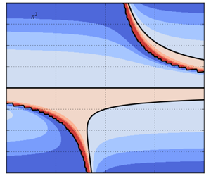
 $$\begin{eqnarray}n^{2}=\frac{\unicode[STIX]{x1D6FD}+k_{d}^{2}U_{0}}{U_{0}-c}-k^{2}-k_{d}^{2}\end{eqnarray}$$
is the refractive index; wave-like solutions require  $0<n^{2}<\infty$, whereas waves are evanescent for
 $n^{2}<0$. The former inequality may be rearranged for a constraint on the zonal phase speed of a wave,
 $U_{0}-(\unicode[STIX]{x1D6FD}+k_{d}^{2}U_{0})/(k^{2}+k_{d}^{2})<c<U_{0}$. The upper limit, where the phase speed approaches the background flow speed, corresponds to a critical layer, whereas the lower limit corresponds to a turning line, a region which Rossby waves refract away from, back towards regions of larger
 $n^{2}$ (O’Rourke & Vallis Reference O’Rourke and Vallis2013; Hoskins & Ambrizzi Reference Hoskins and Ambrizzi1993). The refractive index may be derived for background flows with general meridional dependence, such that the above inequality becomes a local constraint on the zonal phase speed, rather than a global one.
In figure 11 we plot the refractive index,  $n^{2}$, versus background flow and zonal wavenumber. By considering the refractive index we are able to understand why a particular background flow permits excitation of Rossby waves across only a specific range of zonal wavenumbers, and, furthermore, why we observe the eigenmode decomposition power distribution shown in figure 10. For example, when
 $U_{0}=U_{e}$, the forcing is unable to excite positive zonal wavenumbers close to and smaller than
 $k=10$, as it is ‘blocked’ by a critical line, on the other side of which
 $n^{2}$ is negative. For
 $U_{0}=U_{w}$, however, the plunger is free to excite a wider range of wavenumbers with positive
 $n^{2}$ values, and therefore does so, resulting in a stronger flow response.
Refractive index,  $n^{2}$, plotted against uniform zonal background flow,
 $U_{0}$, and zonal wavenumber,
 $k$. Positive
 $n^{2}$ values are required for wave-like solutions to exist for a given background flow and wavenumber. In negative regions, waves are evanescent (O’Rourke & Vallis Reference O’Rourke and Vallis2013). Black lines illuminate zero-value contours, which are either a critical layer or a turning line.

4.3 Wavenumber properties and redistribution efficiency
In this subsection we consider the wavenumber properties of the excited Rossby wave spectrum and use this to define a novel measure of redistribution efficiency. To do this, we use the notion that waves with zonal and meridional wavenumbers,  $k$ and
 $l$, such that
 $|k|=|l|$ are those that most efficiently drive eastward momentum flux convergence at their source. We know the zonal wavenumber of each of our eigenmodes, but we do not currently have a corresponding meridional wavenumber. To find this, we use the SSH component of the eigenmode and find its dominant meridional length scale. Thus, we define the meridional pseudo-wavenumber of eigenmode
 $\unicode[STIX]{x1D74D}_{i,j}$ as
 $$\begin{eqnarray}\hat{l}_{i,j}=\text{max}_{l\in \left\{0,\ldots ,(N-1)/2\right\}}\left(|{\mathcal{F}}_{y}[h_{0}](l)|+|{\mathcal{F}}_{y}[h_{0}](-l)|\right),\end{eqnarray}$$
where  ${\mathcal{F}}_{y}[\cdot ]$ is the meridional Fourier transform operator. Here,
 $h_{0}$ is the physical-space representation of the SSH component of the eigenmode in question, evaluated at an arbitrary instant in time,
 $t_{0}$, and longitude,
 $x_{0}$. That is, given the SSH component of an eigenmode,
 $\tilde{h}$, we have
 $$\begin{eqnarray}h_{0}=Re\left[{\mathcal{F}}_{x}^{-1}[\tilde{h}]\exp \left(-2\unicode[STIX]{x03C0}\text{i}\unicode[STIX]{x1D714}t\right)\right](x_{0},y,t_{0}),\end{eqnarray}$$
where  ${\mathcal{F}}_{x}^{-1}[\cdot ]$ is the inverse zonal Fourier transform operator. The definition of the meridional pseudo-wavenumber (4.11) selects the wavenumber corresponding to the dominant meridional length scale in the SSH field. We use free-slip boundary conditions, but for no-slip conditions there is a tendency for modes to be oscillatory near the boundaries, which equates to a tendency for (4.11) to select larger wavenumbers. Thus, in order to produce the same results when using no-slip boundary conditions, extra care has to be taken to filter out the influence by this oscillatory behaviour.
For each mode we now have zonal and meridional wavenumbers, and the corresponding frequency. Before defining a measure for redistribution efficiency, this triplet can be compared with expectations from Rossby wave theory. We make use of the viscous Rossby wave dispersion relation, found by seeking wave-like solutions to the linearised QG equation (4.8),
 $$\begin{eqnarray}\unicode[STIX]{x1D714}=U_{0}k-\frac{\unicode[STIX]{x1D6FD}k}{K^{2}}-\text{i}\unicode[STIX]{x1D6FE}-\text{i}\unicode[STIX]{x1D708}K^{2},\end{eqnarray}$$
where  $K^{2}=k^{2}+l^{2}$. To simplify the algebra we have neglected the inverse deformation radius term, which is extremely small and does not influence the results. To comply with standard notation, we briefly use cyclic wavenumbers so that they incorporate the factor of
 $2\unicode[STIX]{x03C0}$. When plotting, we ensure that wavenumbers are represented in their non-cyclic form. Equation (4.13) can be rearranged for an expression for the meridional wavenumber
 $l$:
 $$\begin{eqnarray}l^{2}=\frac{1}{2\text{i}\unicode[STIX]{x1D708}}\left[-\unicode[STIX]{x1D6FF}-\text{i}\left(2\unicode[STIX]{x1D708}k^{2}+\unicode[STIX]{x1D6FE}\right)\pm \sqrt{(\unicode[STIX]{x1D6FF}+\text{i}\unicode[STIX]{x1D6FE})^{2}-4\text{i}\unicode[STIX]{x1D6FD}\unicode[STIX]{x1D708}k}\right],\end{eqnarray}$$
where  $\unicode[STIX]{x1D6FF}=\unicode[STIX]{x1D714}-U_{0}k$. This expression yields four complex
 $l$-values for each set of input parameters. We retain the real part only and omit the negative counterpart of each pair of roots.
In figure 12 we present scatter plots of  $(k,\hat{l})$, where
 $\hat{l}$ is dominant meridional wavenumber of the most dominant mode at wavenumber
 $k$, and where colour corresponds to the periodicity (units days) of the mode. We also plot
 $(k,l)$ as expected from Rossby wave theory using (4.14), for a selection of periodicities (see legend). We show data for both
 $U_{0}=-0.08~\text{m}~\text{s}^{-1}$ and
 $U_{0}=0.08~\text{m}~\text{s}^{-1}$. The wavenumbers of the dominant excited modes are arranged in bands of approximately constant periodicity, and these bands are also produced by the viscous dispersion relation. For each background flow, the strongest modes (see figure 10 for comparison) are those which have periodicity close to the predetermined forcing periodicity,
 $T=60$ days, and have wavenumber values which are also observable in data predicted by the dispersion relation. At larger
 $|k|$, the most dominant modes generally have frequency that does not match the system frequency or an integer multiple of the system frequency. Although an aside to the primary intentions of this study, this represents a significant result in that waves are not exclusively selected by their frequency, but rather can instead be selected due to spatial resonances with the external forcing.
(a,c) Scatter plot of zonal wavenumber  $k$ and meridional pseudo-wavenumber
 $\hat{l}$ for the most dominant mode at wavenumber
 $k$. Colour corresponds to the periodicity of the mode, in units of days. (b,d) Predictions from the Rossby wave dispersion relation; scatter plot of
 $(k,l)$, where
 $l$ is calculated using (4.14). Each colour corresponds to a different periodicity
 $T$. Diamonds correspond to taking the positive root in (4.14), and circles correspond to the negative root. See the legend for reference. In the upper row the background flow is
 $U_{0}=-0.08~\text{m}~\text{s}^{-1}$, whereas in the lower row we have
 $U_{0}=0.08~\text{m}~\text{s}^{-1}$.

The meridional pseudo-wavenumber can be used to define a new measure of redistribution efficiency. We exploit the idea that modes with wavenumbers such that  $\hat{l}=|k|$ are those that most efficiently redistribute zonal momentum, since they have phase lines tilted close to the basin diagonal and have purely meridional group velocity. Since our flow response is a superposition of many such waves, we also want a measure to take into account each mode and its corresponding amplitude. This motivates the following definition of the wave efficiency:
 $$\begin{eqnarray}e=\frac{\displaystyle \mathop{\sum }_{i,j}|\unicode[STIX]{x1D703}_{i,j}|}{\displaystyle \mathop{\sum }_{i,j}\left|\left|k_{i}\right|-\hat{l}_{i,j}\right|\cdot \left|\unicode[STIX]{x1D703}_{i,j}\right|},\end{eqnarray}$$
with the wavenumber dependence in the denominator so that larger  $e$-values correspond to a more efficient flow response. The numerator acts to normalise the measure so that it has no dependence on the total amplitude of the flow response. Figure 13 plots the wave efficiency against uniform zonal background flow
 $U_{0}$, which should be compared with the plot of the alternative efficiency measure,
 $\hat{{\mathcal{M}}}_{0}$ (figure 9a). First, note that we reproduce the bimodal structure, with maxima for
 $U_{0}\approx U_{w}$ and
 $U_{0}\approx U_{e}$. Furthermore, this measure implies that the flow is more efficient for zonal momentum redistribution for
 $U_{0}\approx U_{w}$ rather than
 $U_{0}\approx U_{e}$, also agreeing with
 ${\mathcal{M}}_{0}$. This measure is closely related to the Rossby wave group velocity, which we consider in the next subsection.
Plot of the wave efficiency measure,  $e$, versus uniform zonal background flow
 $U_{0}$ (units m s
 $^{-1}$). Note that the
 $y$-axis range begins at a non-zero value.

4.4 Insights from group velocities
Here, we consider the group velocity property of excited Rossby waves, which provides a deeper insight into the amplitude of the zonal momentum redistribution. Using the quasi-geostrophic approximation, the zonal and meridional group velocity components are
 $$\begin{eqnarray}c_{g}^{x}=U_{0}+\frac{\unicode[STIX]{x1D6FD}\left(k^{2}-l^{2}\right)}{\left(k^{2}+l^{2}\right)^{2}}\quad \text{and}\quad c_{g}^{y}=\frac{2\unicode[STIX]{x1D6FD}kl}{\left(k^{2}+l^{2}\right)^{2}},\end{eqnarray}$$
respectively. To find the group velocity of an eigenmode, we may replace the meridional wavenumber,  $l$, with the meridional pseudo-wavenumber,
 $\hat{l}$. In our plunger-induced flow response, the meridional group velocity is, generally, southwards/northwards to the south/north of the plunger, which, for a given
 $k$, is determined by the sign of
 $l$. Although we have imposed that the meridional pseudo-wavenumber of an eigenmode is non-negative, this does not pose a problem since our main interest is the amplitude of the meridional group velocity. Similar to the wave efficiency measure (equation (4.15)), we can define measures of the effective group speed of a flow response by taking weighted mean of
 $c_{g}^{x}$ and
 $c_{g}^{y}$. Denoting
 $c_{g,i,j}^{x}$ and
 $c_{g,i,j}^{y}$ as the group velocity components for mode
 $(i,j)$, we define the effective group velocity components as
 $$\begin{eqnarray}c_{g,eff}^{x}=\frac{\displaystyle \mathop{\sum }_{i,j}\,|\unicode[STIX]{x1D703}_{i,j}|\,c_{g,i,j}^{x}}{\displaystyle \mathop{\sum }_{i,j}|\,\unicode[STIX]{x1D703}_{i,j}|}\quad \text{and}\quad c_{g,eff}^{y}=\frac{\displaystyle \mathop{\sum }_{i,j}\,|\unicode[STIX]{x1D703}_{i,j}|\,c_{g,i,j}^{y}}{\displaystyle \mathop{\sum }_{i,j}|\,\unicode[STIX]{x1D703}_{i,j}|}.\end{eqnarray}$$
In figure 14 we plot the (adjusted, see caption) effective group velocity components versus  $U_{0}$. As discussed in Waterman & Jayne (Reference Waterman and Jayne2012), we expect Rossby waves with purely meridional group velocity to be the most efficient in driving zonal momentum flux convergence at the Rossby wave source. This is indeed reflected in the effective group velocities, with the amplitude of the meridional component maximised for
 $U_{0}\approx U_{w}$, at which point the zonal component is minimised.
Absolute value of the effective meridional group speed ( $|c_{g,eff}^{y}|$, blue line), and the effective zonal group speed minus the background flow (
 $c_{g,eff}^{x}-U_{0}$, green line), plotted against uniform zonal background flow. We subtract
 $U_{0}$ from
 $c_{g,eff}^{x}$ so as to more easily visualise its variation with respect to
 $U_{0}$. Units for both axes are
 $\text{m}~\text{s}^{-1}$.

4.5 Section summary and comparison with previous results
The results of this section compliment the results of § 3 in that they provide distinct measures of the two factors – resonance and redistribution efficiency – that contribute to the zonal momentum redistribution profile shown in figure 8. The total power in the eigenmode decomposition for a given  $U_{0}$ quantifies the resonance between the plunger forcing and the Rossby wave spectrum. Plotted against
 $U_{0}$ (figure 10), this measure resembles the bimodal structure of the total kinetic energy,
 ${\mathcal{K}}$ (which scales with the square of the flow amplitude). We can further conclude that increased/decreased resonance is due to a wide/narrow range of available zonal wavenumbers for a particular background flow, as is predicted by the refractive index (figure 11) and quantified by the decomposition weights (figure 10). Eddy zonal momentum flux convergence at the forced latitude,
 $y_{0}$, is driven by Rossby waves propagating away from their source, carrying with them westward momentum. Waves that are most efficient at driving eastward mean flows at their source are those that have purely meridional group velocity. From the meridional and zonal group velocity estimates (figure 14), we infer that
 $U_{0}\approx U_{w}$ is the background flow for which the excited Rossby waves have group velocity closest to being purely meridional. On the other hand, for weak eastward background flow, for which the group speed is close to being zonal, we have only weak zonal momentum flux convergence at
 $y_{0}$. These results are also quantified by the two measures of redistribution efficiency (figures 13 and 9).
As discussed in § 3, the group velocity is parallel (for non-divergent velocity field and zero background PV gradient) to the vector of eddy anisotropy and tilt parameters,  $E=-(M,N)$, which provides a link between the Rossby wave description and the local eddy geometry description. Moreover, in the zonal-mean framework, the zonal momentum redistribution is equal to meridional derivative of the eddy tilt parameter. For a fixed kinetic energy density, the eddy tilt
 $N$ is maximised for a wavenumber pair with
 $|k|=|l|$, which corresponds to a purely meridional group velocity and phase lines tilted
 $45$ degrees to the horizontal. An important point to note is that the meridional scale of the excited flow response varies little as the background flow is altered, such that large
 $N$ corresponds to proportionally large
 $N_{y}$. Thus, the dominant effect of varying the background flow is to adjust the spectrum of excited zonal wavenumbers. We then observe maximal zonal momentum redistribution for
 $U_{0}=U_{w}$ for two reasons: (i) a wide range of zonal wavenumbers available for excitement (resonance) and (ii) a large quantity of available waves which have
 $|k|\sim |l|$ (redistribution efficiency).
5 Discussion
The aim of this study was to develop a deep understanding of the excitation and self-interaction of Rossby waves in the single-layer rotating shallow-water system. We excite Rossby waves via a localised plunger forcing, intended to be an elementary representation of transient eddy flux divergences, and is motivated by the need to understand mean-flow generation by transient disturbances (e.g. Haidvogel & Rhines (Reference Haidvogel and Rhines1983) and Waterman & Hoskins (Reference Waterman and Hoskins2013)). We quantify the mean-flow generation associated with the plunger, and the induced Rossby wave field, by using the time-mean eddy zonal momentum flux convergence (zonal momentum redistribution). Since the governing system is linear, this involves use of the quasi-nonlinear approximation, in which nonlinear flux terms are evaluated from linear dynamics (Berloff & Kamenkovich Reference Berloff and Kamenkovich2013a,Reference Berloff and Kamenkovichb; Berloff Reference Berloff2015; Haigh & Berloff Reference Haigh and Berloff2018), and are purely diagnostic. It can be shown via perturbation analysis (Mizuta Reference Mizuta2018a,Reference Mizutab) that the self-interaction of the linear flow response is the primary driver of momentum and potential vorticity fluxes near the surface, with higher-order terms playing a less prevalent role.
We have concentrated on the role of a uniform zonal background flow,  $U_{0}$, and consistently observe convergence of eddy zonal momentum fluxes, i.e. eastward mean-flow generation, at the forced latitudes, with westward recirculation zones to the north and south (and slightly downstream). Moreover, we observe a robust and significant dependence on the amplitude and direction of the background flow, with, for example, maximal zonal momentum redistribution attained for weak westward
 $U_{0}$. We have shown that this dependence is due to the nature of the excited Rossby wave field: the amplitude, quantity and wavenumber properties of the involved waves dictate the amplitude of the flow response and the efficiency of zonal momentum redistribution.
The plunger forcing used in our study may be broadly interpreted as any source of oceanic Rossby wave activity. For example, in the real oceans it is understood that meanders of eastward jets radiate Rossby waves (Pedlosky Reference Pedlosky1977; Mizuta Reference Mizuta2009), and the results of the present study are applicable in this context. Diagnostics of our idealised simulations exhibit eastward momentum flux convergence at the forced latitudes, which corresponds to a northward flux of PV and is consistent with the PV/zonal momentum structure of an oceanic eastward jet extension (Waterman & Jayne Reference Waterman and Jayne2012). Furthermore, for a physically reasonable forcing amplitude and corresponding instantaneous velocity response on the dimensional order of  $0.01~\text{m}~\text{s}^{-1}$, the time-integrated (over
 $60$ days) eddy zonal momentum flux convergence is of the order of
 $1~\text{m}~\text{s}^{-1}$, and is therefore significant with regards to the driving of large-scale mean flows.
The amplitude of the zonal momentum redistribution, and its dependence on the uniform zonal background flow, can be applied towards a parameterisation of mesoscale eddies using the method of Berloff (Reference Berloff2015), hereafter B15. B15 considers the plunger-induced PV flux convergence in the QG system, and quantifies its dependence on uniform background flow. This dependence is then used to scale a set of external dipole inputs of PV which are included in a non-eddy-resolving QG double-gyre simulation. The resulting simulation, with eddy effects now parameterised, closely resembles the large-scale component of the reference eddy-resolving simulation, and recovers a coherent eastward jet extension which was previously absent. An important quality of this method is its innate ability to capture up-gradient fluxes of PV or momentum, whereas the commonly employed down-gradient diffusion (Gent (Reference Gent2011) argues that the parameterisation of Gent & McWilliams (Reference Gent and McWilliams1990) ought to be interpreted as an extra advection term, although it has a diffusive effect on isopycnal surfaces.) parameterisation of Gent & McWilliams (Reference Gent and McWilliams1990), which is often implemented with a constant diffusivity, is not able to capture this process. An extension of the present study is therefore to apply its methods and extend results towards a parameterisation of mesoscale eddies for use in primitive-equation ocean models.
Another extension to this study could be to overcome the quasi-nonlinear approach by implementing a nonlinear SW model and re-analysing the plunger-induced Rossby waves and associated mean-flow generation. It is hypothesised that the same qualitative behaviour will be observed, just as it is in the nonlinear quasi-geostrophic model (Haidvogel & Rhines Reference Haidvogel and Rhines1983; Waterman & Jayne Reference Waterman and Jayne2012) and primitive-equation model (Mizuta Reference Mizuta2018a). It may also be worthwhile to introduce the effects of baroclinicity via the use of the two- or three-layer SW equations, and consider plunger forcing in these systems. A particular challenge in this vein regards defining the forcing regime, as it not clear what the qualitative structure of the forcing should be, and is further complicated by the presence of three prognostic variables in each layer (as opposed to one per layer in the QG approximation). With a multi-layer system, we can model fluxes at depth, as well as near the surface. The numerical simulations of Holland & Rhines (Reference Holland and Rhines1980) predict southward PV fluxes at depth, but Mizuta (Reference Mizuta2018a) predicts that this is not driven by the self-interaction of the linear flow response, but rather by the self-interaction of nonlinear terms.
Acknowledgements
M.H. is funded by the UK Engineering and Physical Sciences Research Council (EPSRC) Centre for Doctoral Training in Mathematics of Planet Earth. P.B. is supported by the NERC grants NE/R011567/1 and NE/T002220/1, the Royal Society Exchange Grant IEC/R2/181033 and the Leverhulme grant RPG-2019-024. The authors are grateful to the anonymous reviewers for their thoughtful and useful comments.
Declaration of interests
The authors report no conflict of interest.



