2 Problem formulation

Consider the steady, two-dimensional flow of a fluid confined in a channel bounded by two parallel walls extending to $\pm \infty$ in the $x$ -direction and driven by a pressure gradient (see figure 1). The gravitational acceleration $g^{\ast }$ is acting in the negative $y$ -direction, the fluid is incompressible, Newtonian, and has thermal conductivity $k^{\ast }$ , specific heat $c^{\ast }$ , thermal diffusivity $\unicode[STIX]{x1D705}^{\ast }=k^{\ast }/\unicode[STIX]{x1D70C}^{\ast }c^{\ast }$ , kinematic viscosity $\unicode[STIX]{x1D708}^{\ast }$ , dynamic viscosity $\unicode[STIX]{x1D707}^{\ast }$ and thermal expansion coefficient $\unicode[STIX]{x1D6E4}^{\ast }$ and variations of the density $\unicode[STIX]{x1D70C}^{\ast }$ follow the Boussinesq approximation. Here asterisks denote dimensional quantities. The velocity field, pressure field and flow rate in the isothermal channel have the form

(2.1a-c ) $$\begin{eqnarray}\boldsymbol{v}_{0}(x,y)=[u_{0}(y),0]=[1-y^{2},0],\quad p_{0}(x,y)=-2x/Re,\quad Q_{0}=4/3,\end{eqnarray}$$

where the channel half-height $h^{\ast }$ has been used as the length scale, $\boldsymbol{v}_{0}(x,y)=[u_{0},v_{0}]$ denotes the velocity vector scaled with the maximum of the $x$ -velocity $U_{max}^{\ast }$ , $p_{0}$ stands for the pressure scaled with $\unicode[STIX]{x1D70C}^{\ast }U_{max}^{\ast 2}$ and the Reynolds number is defined as $Re=U_{max}^{\ast }h^{\ast }/\unicode[STIX]{x1D708}^{\ast }$ .

Figure 1.

Schematic diagram of the flow system.

The lower wall is heated resulting in its temperature $T_{L}^{\ast }$ varying periodically in $x^{\ast }$ with wavelength $\unicode[STIX]{x1D706}^{\ast }=2\unicode[STIX]{x03C0}/\unicode[STIX]{x1D6FC}^{\ast }$ , where $\unicode[STIX]{x1D6FC}^{\ast }$ is the wavenumber, while the upper wall is isothermal and kept at temperature $T_{U}^{\ast }$ . We define the relative temperature $\unicode[STIX]{x1D703}^{\ast }=T^{\ast }-T_{U}^{\ast }$ , resulting in boundary temperatures of the form

(2.2a,b ) $$\begin{eqnarray}\unicode[STIX]{x1D703}_{L}^{\ast }(x^{\ast })=\unicode[STIX]{x1D703}_{uni}^{\ast }+\unicode[STIX]{x1D703}_{p}^{\ast }\mathop{\sum }_{n=-\infty ,n\neq 0}^{n=+\infty }[\unicode[STIX]{x1D703}_{p}^{(n)\ast }/\unicode[STIX]{x1D703}_{p}^{\ast }]\text{e}^{\text{i}n\unicode[STIX]{x1D6FC}^{\ast }x^{\ast }},\quad \unicode[STIX]{x1D703}_{U}(x^{\ast })=0,\end{eqnarray}$$

where $L$ and $U$ refer to the lower and upper walls, respectively, $\unicode[STIX]{x1D703}_{uni}^{\ast }=T_{mean,L}^{\ast }-T_{U}^{\ast }$ , $\unicode[STIX]{x1D703}_{p}^{\ast }$ is the difference between the maximum and minimum of the lower-wall temperature and $\unicode[STIX]{x1D703}_{p}^{(n)\ast }$ are the complex amplitudes of the Fourier modes required to describe spatial temperature variations. These amplitudes satisfy the reality condition, which requires that $\unicode[STIX]{x1D703}_{p}^{(n)\ast }$ and $\unicode[STIX]{x1D703}_{p}^{(-n)\ast }$ are complex conjugates. Use of $\unicode[STIX]{x1D705}^{\ast }\unicode[STIX]{x1D708}^{\ast }/(g^{\ast }\unicode[STIX]{x1D6E4}^{\ast }h^{\ast 3})$ as the temperature scale results in the following dimensionless expressions for the wall temperatures:

(2.3a,b ) $$\begin{eqnarray}\unicode[STIX]{x1D703}_{L}(x)=Ra_{uni}+Ra_{p}\mathop{\sum }_{n=-\infty ,n\neq 0}^{n=+\infty }\unicode[STIX]{x1D703}_{p}^{(n)}\text{e}^{\text{i}n\unicode[STIX]{x1D6FC}x},\quad \unicode[STIX]{x1D703}_{U}(x)=0,\end{eqnarray}$$

where $Ra_{uni}=g^{\ast }\unicode[STIX]{x1D6E4}^{\ast }h^{\ast 3}\unicode[STIX]{x1D703}_{uni}^{\ast }/(\unicode[STIX]{x1D705}^{\ast }\unicode[STIX]{x1D708}^{\ast })$ and $Ra_{p}=g^{\ast }\unicode[STIX]{x1D6E4}^{\ast }h^{\ast 3}\unicode[STIX]{x1D703}_{p}^{\ast }/(\unicode[STIX]{x1D705}^{\ast }\unicode[STIX]{x1D708}^{\ast })$ are the uniform and periodic Rayleigh numbers. All material properties used in these expressions are to be evaluated at the upper-wall temperature  $T_{U}^{\ast }$ .

The flow in the heated channel is described by the continuity, Navier–Stokes and energy equations of the form

(2.4a,b ) $$\begin{eqnarray}\frac{\unicode[STIX]{x2202}u}{\unicode[STIX]{x2202}x}+\frac{\unicode[STIX]{x2202}v}{\unicode[STIX]{x2202}y}=0,\quad u\frac{\unicode[STIX]{x2202}u}{\unicode[STIX]{x2202}x}+v\frac{\unicode[STIX]{x2202}u}{\unicode[STIX]{x2202}y}=-\frac{\unicode[STIX]{x2202}p}{\unicode[STIX]{x2202}x}+\unicode[STIX]{x1D6FB}^{2}u,\end{eqnarray}$$

(2.4c,d ) $$\begin{eqnarray}u\frac{\unicode[STIX]{x2202}v}{\unicode[STIX]{x2202}x}+v\frac{\unicode[STIX]{x2202}v}{\unicode[STIX]{x2202}y}=-\frac{\unicode[STIX]{x2202}p}{\unicode[STIX]{x2202}y}+\unicode[STIX]{x1D6FB}^{2}v+Pr^{-1}\unicode[STIX]{x1D703},\quad u\frac{\unicode[STIX]{x2202}\unicode[STIX]{x1D703}}{\unicode[STIX]{x2202}x}+v\frac{\unicode[STIX]{x2202}\unicode[STIX]{x1D703}}{\unicode[STIX]{x2202}y}=Pr^{-1}\unicode[STIX]{x1D6FB}^{2}\unicode[STIX]{x1D703},\end{eqnarray}$$

$u,v$

$x,y$

$U_{v}^{\ast }=\unicode[STIX]{x1D708}^{\ast }/h^{\ast }$

$p$

$\unicode[STIX]{x1D70C}^{\ast }U_{v}^{\ast 2}$

$Pr=\unicode[STIX]{x1D708}^{\ast }/\unicode[STIX]{x1D705}^{\ast }$

(2.5a-d ) $$\begin{eqnarray}u(x,-1)=u(x,1)=0,\quad v(x,-1)=v(x,1)=0,\quad \unicode[STIX]{x1D703}(x,-1)=\unicode[STIX]{x1D703}_{L}(x),\quad \unicode[STIX]{x1D703}(x,1)=0.\end{eqnarray}$$

The relation between the heating and the pressure losses is quantified by comparing pressure gradients required to drive the same flow rate through the isothermal and heated channels. This gradient in the case of the heated channel can be written as

(2.6) $$\begin{eqnarray}\left.\frac{\unicode[STIX]{x2202}p}{\unicode[STIX]{x2202}x}\right|_{mean}=Re(-2+A/Re),\end{eqnarray}$$

where a positive value of the correction $A$ identifies reduction of pressure losses. To make this comparison meaningful, one must impose the fixed flow rate constraint of the form

(2.7) $$\begin{eqnarray}Q=\int _{-1}^{1}u\,\text{d}y=\frac{4}{3}Re\end{eqnarray}$$

on the solution of the flow problem.

System (2.3)–(2.6) can be expressed in terms of the stream function defined in the usual manner, i.e. $u=\unicode[STIX]{x2202}\unicode[STIX]{x1D713}/\unicode[STIX]{x2202}y$ , $v=-\unicode[STIX]{x2202}\unicode[STIX]{x1D713}/\unicode[STIX]{x2202}x$ , and normalized with condition $\unicode[STIX]{x1D713}(-1)=0$ , resulting in a problem of the form

(2.8a,b ) $$\begin{eqnarray}\unicode[STIX]{x1D6FB}^{4}\unicode[STIX]{x1D713}-Pr^{-1}\frac{\unicode[STIX]{x2202}\unicode[STIX]{x1D703}}{\unicode[STIX]{x2202}x}=N_{VV},\quad \unicode[STIX]{x1D6FB}^{2}\unicode[STIX]{x1D703}=Pr\,N_{V\unicode[STIX]{x1D703}},\end{eqnarray}$$

(2.8c-g ) $$\begin{eqnarray}\unicode[STIX]{x1D713}(x,-1)=0,\quad \unicode[STIX]{x1D713}(x,1)=\frac{4}{3}Re,\quad \left.\frac{\unicode[STIX]{x2202}\unicode[STIX]{x1D713}}{\unicode[STIX]{x2202}y}\right|_{(x,y=\pm 1)}=0,\quad \unicode[STIX]{x1D703}(x,-1)=\unicode[STIX]{x1D703}_{L}(x),\quad \unicode[STIX]{x1D703}(x,1)=0,\end{eqnarray}$$

$N_{VV}$

$N_{V\unicode[STIX]{x1D703}}$

(2.9a,b ) $$\begin{eqnarray}N_{VV}=\frac{\unicode[STIX]{x2202}}{\unicode[STIX]{x2202}y}\left(\frac{\unicode[STIX]{x2202}}{\unicode[STIX]{x2202}x}\widehat{uu}+\frac{\unicode[STIX]{x2202}}{\unicode[STIX]{x2202}y}\widehat{uv}\right)-\frac{\unicode[STIX]{x2202}}{\unicode[STIX]{x2202}x}\left(\frac{\unicode[STIX]{x2202}}{\unicode[STIX]{x2202}x}\widehat{uv}+\frac{\unicode[STIX]{x2202}}{\unicode[STIX]{x2202}y}\widehat{vv}\right),\quad N_{V\unicode[STIX]{x1D703}}=\frac{\unicode[STIX]{x2202}}{\unicode[STIX]{x2202}x}\widehat{u\unicode[STIX]{x1D703}}+\frac{\unicode[STIX]{x2202}}{\unicode[STIX]{x2202}y}\widehat{v\unicode[STIX]{x1D703}},\end{eqnarray}$$

with symbol $\widehat{ab}$ denoting a product of functions $a$ and  $b$ . The $x$ -dependence of the flow quantities is captured by expressing them as Fourier expansions of the form

(2.10a-c ) $$\begin{eqnarray}\unicode[STIX]{x1D713}(x,y)=\mathop{\sum }_{n=-\infty }^{n=+\infty }\unicode[STIX]{x1D711}^{(n)}(y)\text{e}^{\text{i}n\unicode[STIX]{x1D6FC}x},\quad u(x,y)=\mathop{\sum }_{n=-\infty }^{n=+\infty }u^{(n)}(y)\text{e}^{\text{i}n\unicode[STIX]{x1D6FC}x},\quad v(x,y)=\mathop{\sum }_{n=-\infty }^{n=+\infty }v^{(n)}(y)\text{e}^{\text{i}n\unicode[STIX]{x1D6FC}x},\end{eqnarray}$$

(2.10d,e ) $$\begin{eqnarray}\unicode[STIX]{x1D703}(x,y)=\mathop{\sum }_{n=-\infty }^{n=+\infty }\emptyset ^{(n)}(y)\text{e}^{\text{i}n\unicode[STIX]{x1D6FC}x},\quad p(x,y)=Ax+\mathop{\sum }_{n=-\infty ,}^{n=+\infty }p^{(n)}(y)\text{e}^{\text{i}n\unicode[STIX]{x1D6FC}x},\end{eqnarray}$$

(2.10f,g ) $$\begin{eqnarray}N_{VV}(x,y)=\mathop{\sum }_{n=-\infty }^{n=+\infty }N_{VV}^{(n)}(y)\text{e}^{\text{i}n\unicode[STIX]{x1D6FC}x},\quad N_{V\unicode[STIX]{x1D703}}(x,y)=\mathop{\sum }_{n=-\infty }^{n=+\infty }N_{V\unicode[STIX]{x1D703}}^{(n)}(y)\text{e}^{\text{i}n\unicode[STIX]{x1D6FC}x}\end{eqnarray}$$

$A$

The mean horizontal pressure gradient is required to overcome frictional resistance. The shear stresses as well as the shear forces per unit length and width of the channel acting on the fluid at the walls have the forms

(2.11a-d ) $$\begin{eqnarray}\unicode[STIX]{x1D70F}_{L}=\left.-\frac{\text{d}u}{\text{d}y}\right|_{y=-1},\quad \unicode[STIX]{x1D70F}_{U}=\left.\frac{\text{d}u}{\text{d}y}\right|_{y=1},\quad F_{L}=\unicode[STIX]{x1D706}^{-1}\int _{0}^{\unicode[STIX]{x1D706}}\unicode[STIX]{x1D70F}_{L}\,\text{d}x,\quad F_{U}=\unicode[STIX]{x1D706}^{-1}\int _{0}^{\unicode[STIX]{x1D706}}\unicode[STIX]{x1D70F}_{U}\,\text{d}x,\end{eqnarray}$$

where $\unicode[STIX]{x1D70F}$ stands for the shear stress scaled with $\unicode[STIX]{x1D70C}^{\ast }U_{v}^{\ast 2}$ , $F$ stands for the shear force scaled in the same manner and subscripts $U$ and $L$ refer to the upper and lower walls, respectively. The shear and pressure forces must balance each other, i.e.

(2.12) $$\begin{eqnarray}(F_{L}+F_{U})=\left.2\frac{\unicode[STIX]{x2202}p}{\unicode[STIX]{x2202}x}\right|_{mean}.\end{eqnarray}$$

It remains to be determined if heating leads to a reduction of the mean pressure gradient or, in other words, a reduction of the mean shear stress.

3 Experimental set-up and procedure

A special experimental facility using air as the working medium (see figure 2) was developed to investigate heating effects. The test rig has the form of a 3 m long rectangular channel with a height of $2h^{\ast }=20$  mm and width $s^{\ast }=420$  mm giving a cross-sectional aspect ratio of $s^{\ast }/(2h^{\ast })=21$ . The channel is tall enough to provide optical access required for non-intrusive velocity measurements. A Cartesian reference system consisting of the streamwise $x$ -, transverse $y$ - and spanwise $z$ -coordinates with the origin at the middle of the channel at the $x$ -location corresponding to the middle of the first heating element is used to describe the system geometry. The channel is mounted horizontally using a laser level. The flow is driven by a piston installed upstream of the test section whose motion is controlled using a ball screw driven by a servo-motor. The speed of the piston can be adjusted digitally, permitting reaching the target velocity with an accuracy of 0.41 %.

Figure 2.

Sketch of the experimental apparatus (all dimensions are in mm).

The piston creates a plug flow with a well-defined mass flow rate which is then converted through viscous friction into fully developed Poiseuille flow downstream from the piston. Formation of Poiseuille flow is analogous to that found in the channel entrance flow problem. It is known that the entry length is minimal for low- $Re$ flows (Sadri & Floryan Reference Sadri and Floryan2002a ,Reference Sadri and Floryan b ; Asai & Floryan Reference Asai and Floryan2004). The proper establishment of Poiseuille flow has been verified experimentally using the test facility with heating turned off, as illustrated in figure 3. The maximum (centre) velocity was found to be $U_{max}^{\ast }=1.6$ , 3.3, 4.9, 8.1, 11.4, 16.3, $24.4~\text{mm}~\text{s}^{-1}$ at $Re=1$ , 2, 3, 5, 7, 10, 15, respectively.

Figure 3.

Streamwise velocity profiles in the isothermal channel at $x=75$ , $z=0$ .

The lower wall is equipped with a set of transverse aluminium pipes carrying hot and cold water coming from baths whose temperatures can be controlled with a resolution of 0.1 K. These pipes are covered with 0.2 mm thick stone paper and provide means for the establishment of a streamwise-periodic temperature distribution at the surface. The wavelength of temperature variations is $\unicode[STIX]{x1D706}^{\ast }=66$  mm, giving a wavenumber $\unicode[STIX]{x1D6FC}=2\unicode[STIX]{x03C0}h^{\ast }/\unicode[STIX]{x1D706}^{\ast }=0.95$ . A total of 16 heating periods was used, with most of the observations made around the 11th period ( $70\leqslant x\leqslant 81$ ). The upper wall was made of 5 mm thick aluminium plate with transverse aluminium pipes carrying water of a specified temperature attached to its external surface providing means for maintaining isothermal conditions. The apparatus creates a two-dimensional $x$ -periodic temperature of the lower wall as illustrated in figures 4 and 5, with the spanwise temperature variations being within $\pm 0.5$  K at $x=72.6$ .

Figure 4.

Contour map of the lower-wall temperature for $Ra_{p}=3500$ .

Figure 5.

Streamwise variations of the bottom-wall temperature for $Ra_{p}=3500$ . (a) Experimental data for three spanwise locations (○, $z=0$ ; ▫, $z=10$ ; ▵, $z=-10$ ). (b) Temperature distribution at $72.6\leqslant x\leqslant 79.2$ and $z=0$ , and its Fourier representation (○, experiments; solid line, Fourier representation).

The lower-surface temperature was measured using an infrared thermal imaging camera (Nippon Avionics H2640). Its temperature was also monitored during experiments using sheet-form thermocouples (Chino C060, Type T). Velocity measurements were carried out using a particle image velocimetry (PIV) system (Dantec Dynamic Studio) consisting of a double-pulsed Nd : YAG laser (Quantel Ever Green) and a CCD camera with a resolution of $2048\times 2048$ pixels (Dantec FlowSense EO 4M). A laser light sheet with a thickness of approximately 1 mm was used to illuminate $1~\unicode[STIX]{x03BC}\text{m}$ diameter seeding in the ( $x,y$ )-plane. The photographed area had a size of $(x^{\ast },y^{\ast })=(100~\text{mm},25~\text{mm})$ . The least squares matching algorithm was employed in post-processing. The interrogation size and overlap in the $y$ -direction were $(x,y)=(33,22)$ pixels and 50 %, respectively, giving (37, 37) velocity vectors in the ( $x,y$ )-directions per one period of heating.

In order to determine the sample size $N$ necessary to achieve statistical convergence, preliminary measurements were made for an isothermal channel using different sample sizes in the range of $10\leqslant N\leqslant 100$ (see figure 3). It was found that the velocity profiles were independent of the sample size and the flow rate was within 1 % of the theoretical value of $Q/Re=4/3$ for $N\geqslant 30$ . Thus, $N=50$ was employed in the experiment. The uncertainty of velocity measurements was estimated for each step of the measurement sequence. The accuracy of PIV is limited by several factors, e.g. particle response to fluid motion, position of light sheet, jitter associated with camera and laser response to controlling pulse, distortion of lens and image sensor, size of the interrogation area and image-matching algorithm. The biased error is estimated to be about 0.1 pixels, which is 5 % of typical particle displacement (2 pixels). However, the excellent agreement for the isothermal flow suggests that the biased error in the instrumentation used is smaller than that. The random uncertainty is mainly due to scatter of the measured velocity resulting from particle distribution and/or flow conditions. When we use a 95 % confidence interval, the value of the time-averaged mean streamwise velocity $\overline{u^{\ast }}$ is within the interval of $\overline{u^{\ast }}\pm 1.96(\sqrt{s_{u^{\ast }}/N})$ , where $s_{u^{\ast }}$ is the variance of  $u^{\ast }$ . The relative uncertainties were found to be about $\pm 1\,\%$ of $\overline{u^{\ast }}$ for all measurements which approximately correspond to the size of plotted symbols.

4 Discussion of results

In the experiments reported in this paper, the cold/hot water supplies were adjusted to keep the upper wall at a constant temperature $T_{U}^{\ast }=303.2$  K, a constant peak-to-peak amplitude of temperature variations along the bottom wall at $\unicode[STIX]{x1D703}_{p}^{\ast }=39.8$  K and mean temperature at $T_{mean,L}^{\ast }=302.8$  K. Since matching of the mean temperature of the lower wall with the temperature of the upper wall was difficult, the experiments were carried out with the mean temperature of the bottom wall lower than the temperature of the upper wall giving $\unicode[STIX]{x1D703}_{uni}^{\ast }=T_{mean,L}^{\ast }-T_{U}^{\ast }=-0.4$  K. This arrangement resulted in a periodic Rayleigh number of $Ra_{p}=3500$ and a uniform Rayleigh number of $Ra_{uni}=-35$ . In the following discussion, the temperature maxima and minima are referred to as hot and cold spots, respectively. It was sufficient to use the first 10 modes in (2.3) to describe the streamwise variations of the bottom-wall temperature (see figure 5 b). The corresponding Fourier expansion coefficients are given in table 1.

Table 1.

Fourier coefficients of expansion (2.3) corresponding to the experimental conditions.

Fluid movement results from an interaction/competition between two types of forces, i.e. the externally imposed horizontal pressure gradient and the buoyancy forces. The resulting flow topologies change significantly depending on the relative magnitudes of these forces, as illustrated in figure 6, which displays both experimental and theoretical results. In this figure, the hot spots are always located at $x=72.6$ and 79.2, and the cold spot at $x=75.9$ .

Figure 6.

Comparisons of the theoretical (upper panels) and experimental (lower panels) flow fields for $Re=$ (a) 0, (b) 1, (c) 2, (d) 3, (e) 5, (f) 7, (g) 10, (h) 15. Locations of the hot spots ( $x=72.6$ and 79.2) are identified using solid arrows while location of the cold spot ( $x=75.9$ ) is identified using dotted arrows. Shading in the experimental panels results from smoke visualization. Shading in the theoretical panels changes from the local minimum (darkest) to the local maximum (lightest) of the stream function. For the theoretical results, the thick solid lines represent streamlines, the thin solid lines represent the positive isotherms while the thin dotted lines represent the negative isotherms. For $Re=0$ , 1, the plotted isotherms correspond to $\unicode[STIX]{x1D703}/\unicode[STIX]{x1D703}_{max}=-0.65$ , $-0.45$ , $-0.2$ , $-0.1$ , 0, 0.01, 0.02, 0.04, 0.1, 0.2, 0.3, 0.5, 0.8; for $Re=2$ , 3, $\unicode[STIX]{x1D703}/\unicode[STIX]{x1D703}_{max}=-0.97$ , $-0.65$ , $-0.33$ , $-0.1$ , 0, 0.02, 0.04, 0.1, 0.2, 0.3, 0.4, 0.65; for $Re=5$ , 7, $\unicode[STIX]{x1D703}/\unicode[STIX]{x1D703}_{max}=-0.45$ , $-0.2$ , $-0.06$ , 0, 0.01, 0.04, 0.1, 0.2, 0.3, 0.4, 0.55, 0.8; for $Re=10$ , $\unicode[STIX]{x1D703}/\unicode[STIX]{x1D703}_{max}=-0.45$ , $-0.2$ , $-0.06$ , 0, 0.01, 0.013, 0.06, 0.1, 0.2, 0.3, 0.4, 0.8; for $Re=15$ , $\unicode[STIX]{x1D703}/\unicode[STIX]{x1D703}_{max}=-0.45$ , $-0.2$ , $-0.06$ , 0, 0.01, 0.02, 0.06, 0.1, 0.2, 0.3, 0.8. The thick dashed lines identify isotherms corresponding to $\unicode[STIX]{x1D703}=0$ .

In the case of $Re=0$ , the fluid movement is driven only by buoyancy forces, resulting in a topology consisting of counter-rotating rolls with the fluid moving upwards above the hot spots and downwards above the cold spots (see figure 6 a). The upward movement of the warm plumes is stronger than the downward movement of the cold plumes resulting in the roll centres being attracted towards the hot spots. Heating rather than cooling dominates as the fluid temperature throughout most of the flow domain increases above the mean lower-wall temperature, except in a small zone around the cold spot where the temperature dips below the mean temperature.

A piston forces the fluid to move in the positive $x$ -direction with the flow rate and the Reynolds number dictated by the piston velocity. The velocity field has a typical Poiseuille form upstream of the heated section, as illustrated in figure 3. Figure 6(b) displays the flow topology resulting from the Poiseuille flow with $Re=1$ exposed to heating. One can look at this flow field as resulting from the convection field shown in figure 6(a) modified by the horizontal pressure gradient. The rolls persist in the same locations trapping in their interiors a certain volume of fluid while the remaining fluid, which is pushed to the right by the piston, finds its way through a well-defined stream tube which meanders around the rolls, moving upwards above the hot spots and downwards above the cold spots. The position of the stream tube is kinematically consistent with the rolls’ rotation. The question of interest is whether the pressure gradient required to generate this particular flow rate is larger or smaller than in the isothermal case. The contact between the stream tube and the walls has been largely eliminated which suggests potential reduction of pressure losses, similar to the case of the super-hydrophobic effect (Rothstein Reference Rothstein2010), and this has led to referring to this effect as the super-thermohydrophobic effect (Floryan Reference Floryan2012). The rolls act as ‘bearings’ carrying the stream tube and this should lead to a further reduction of the pressure gradient. The bearings’ rotation is partially driven by the buoyancy force, which should contribute to the reduction of pressure losses, and partially by the shear between the fluid in the stream tube and in the rolls, which should increase the pressure losses. The complex form of the stream tube as well as its length suggests the formation of high shear forces which would increase the drag. The rolls reduce the cross-sectional area available to the flow and this should increase pressure losses. Since all these effects are simultaneously present and oppose each other, determining whether the drag decreases or increases requires detailed analysis. Before proceeding with the rest of the discussion, we point out an excellent agreement between the theoretically and experimentally determined flow fields (see figure 6).

An increase of the horizontal mean pressure gradient while keeping the same heating conditions (the same buoyancy forces) results in an increase of the horizontal flow rate and increase of the Reynolds number. Results for $Re=2$ displayed in figure 6(c) demonstrate the existence of a flow topology qualitatively similar to that for $Re=1$ but with the stream tube becoming wider and straighter as it has to carry a larger flow rate. This process is continued at $Re=3$ (figure 6 d) with the size of the upper rolls decreasing faster than that of the lower rolls. The change in the character of the temperature field is first noticed for $Re=5$ with the colder region extending further in the downstream direction (see figure 6 e). At $Re=10$ (figure 6 g) the upper rolls become marginal and the stream tube occupies most of the channel. At $Re=15$ (figure 6 h), the upper rolls have been eliminated while the lower rolls still exist in a residual form. Further increase of $Re$ eliminates the rolls altogether with the flow topology becoming identical to that found in an isothermal channel (details not shown). The pressure-gradient-driven flow becomes so strong that the buoyancy forces no longer play any role in the fluid movement. In closing this part of the discussion, one should note the downstream movement of the separation point at the lower wall where the stream tube turns upwards; this point moves from $x=72.6$ , which represents the limit for $Re\rightarrow 0$ (no pressure gradient effects), to $x\approx 74$ at $Re=15$ (buoyancy effects are negligible).

It is known that thermal convection flows are highly unstable and tend to break into secondary motions. Results presented in figure 6 demonstrate that the flow is stationary and stable under the conditions used in the experiment and remains two-dimensional. The critical Rayleigh number for the onset of secondary convective motion for unimodal periodic heating is $Ra_{p}\approx 3000$ (Hossain & Floryan Reference Hossain and Floryan2015b ). Its value rises rapidly when the lower-wall mean temperature decreases below the upper-wall temperature ( $Ra_{uni}<0$ ; Hossain & Floryan Reference Hossain and Floryan2017) as is the case in the present experiment. Stability conditions in the case of multimodal heating remain to be determined but, as the current results demonstrate, the flow remains stable at $Ra_{p}=3500$ .

Measurements of the horizontal velocity component were carried out using the non-intrusive PIV technique. It is known that the measurements near the walls are biased due to low-density inhomogeneous seeding, reflection of mirrored images and other technical challenges, as discussed by Kahler, Scharonowski & Cierpka (Reference Kahler, Scharonowski and Cierpka2012). Ideally, the bias errors may be averaged out when the velocity gradient is constant, and particles are seeded homogeneously. In the present flow configuration, however, velocity gradients change drastically in the near-wall region. In addition, the magnitude of the velocity changes significantly as a function of $x$ as $u$ decreases significantly in locations where the vertical roll motion dominates (see figure 6). Results displayed in figure 7 for three illustrative cases, i.e. $Re=0$ , 5 and 15, demonstrate a very good agreement between experimental and theoretical results in the bulk of the flow as well as a reduction of the backward flow as $Re$ increases. The lack of experimental points in the immediate neighbourhoods of the walls is associated with the limitations of the measurement technique.

Figure 7.

Distributions of the horizontal velocity component every $1/8$ of the heating wavelength starting at the hot spot (location 1) for $Re=0$ (a), $Re=5$ (b) and $Re=15$  (c). Locations  $1,2,3,\ldots ,8$ correspond to $x/\unicode[STIX]{x1D706}=0$ , $1/8$ , $1/4$ , $3/8$ , $1/2$ , $5/8$ , $6/8$ , $7/8$ , respectively, where $x=0$ corresponds to the left-hand hot spot in the observation area. Locations 1 and 5 are not shown in (a) as they correspond to the flow moving only in the vertical direction. Symbols identify experimental points while solid lines illustrate theoretical results.

Solutions of the field equations for the heating conditions used in the experiment demonstrate that reduction of pressure losses does occur (see figure 8). The magnitude of the drag reduction is determined by the interplay between the buoyancy forces and the externally imposed horizontal pressure forces. The shift from the former dominating flow at small $Re$ to the latter dominating flow at larger $Re$ takes place at $Re\approx 14$ . The highest reduction in relative terms is achieved at $Re=11$ and it is about 8.5 %. The elimination of the drag-reducing effect for larger $Re$ correlates well with the elimination of convection bubbles. The magnitudes of pressure gradients are extremely small (see table 2) and, thus, the heating-induced changes in pressure drops over the length of the experimental model are not accessible to direct measurements. This necessitates the use of an indirect method.

Figure 8.

Variations of the pressure gradient correction ( $A$ ), the pressure gradient for the isothermal channel ( $B=-2\times Re$ ) and the ratio $A/B$ as functions of the flow Reynolds number.

Table 2.

Variations of the theoretically determined isothermal mean pressure gradient ( $\unicode[STIX]{x2202}p/\unicode[STIX]{x2202}x|_{iso}$ ), isothermal mean shear at the upper $(\unicode[STIX]{x1D70F}_{U,iso})$ and lower $(\unicode[STIX]{x1D70F}_{U,iso})$ walls, mean shear at the lower wall ( $\unicode[STIX]{x1D70F}_{L,mean}$ ), mean shear at the upper wall ( $\unicode[STIX]{x1D70F}_{U,mean}$ ), the pressure gradient correction ( $A$ ) and the same correction expressed as a fraction of the isothermal pressure loss for the Reynolds numbers used in the experiments.

The pressure gradient can be determined from a balance of forces acting on a convenient control volume, i.e. (2.12). Since pressure losses are generated only by wall shear, measurements of shear over one heating wavelength should provide information sufficient for determination of the pressure gradient. The theoretical shear distributions between two adjacent hot spots determined for the experimental conditions are displayed in figure 9. Shear at the lower wall changes direction depending on the position with respect to the convection bubbles. It acts in the positive $x$ -direction in the zone adjacent to the clockwise-rotating bubble and, thus, assists with the fluid movement along the channel, and in the opposite direction in the zone adjacent to the counterclockwise-rotating bubble opposing the fluid movement. The situation at the upper wall is reversed in the sense that shear adjacent to the clockwise-rotating bubble opposes the fluid movement while shear adjacent to the counterclockwise-rotating bubble assists with the fluid movement. This situation is very clear for small $Re$ but becomes more complex with an increase of $Re$ as bubbles decrease in size and their positions shift downstream. The amplitudes of shear variations are very large, especially when compared with the isothermal shear for the upper, $\unicode[STIX]{x1D70F}_{U,iso}$ , and lower, $\unicode[STIX]{x1D70F}_{L,iso}$ , walls (see table 2). The largest magnitudes are observed for $Re=0$ and they decrease with an increase of $Re$ but in a different manner at the upper and lower walls. The maximum at the lower wall starts at around 119 and decreases to 81 when the Reynolds number increases from $Re=0$ to $Re=15$ , while the minimum starts at around $-123$ and increases to $-115$ . At the upper wall, the maximum starts at 156 and decreases to $-5$ , while the minimum starts at $-115$ and increases to $-66$ . Heating always increases the mean shear at the upper wall ( $\unicode[STIX]{x1D70F}_{U,mean}$ ) while it decreases the mean shear at the lower wall ( $\unicode[STIX]{x1D70F}_{L,mean}$ ). This decrease is always larger resulting in an overall reduction of the shear and, thus, reduction of the pressure gradient (see table 2).

Figure 9.

Variations of the theoretically determined wall shear at the lower (a) and upper (b) walls between the hot spots determined for the experimental conditions. The thin dotted lines illustrate the distribution of the lower-wall temperature (not to scale). Here $x=0$ corresponds to the left-hand hot spot in the observation area.

The local values of the wall shear are of the order of $10^{-4}$  Pa which make them difficult to measure directly (Kahler et al. Reference Kahler, Scharonowski and Cierpka2012; Dongqing Li 2015). The mean shear is the difference between the integrals of the local shear over its positive segment, where the local shear may reach values of up to 100, and the negative segment, where the local shear may reach values of up to $-100$ (see figure 9). Accordingly, the local shear must be evaluated very accurately to make the difference between these two integrals meaningful. This shear was determined from the velocity profiles such as those displayed in figure 7.

The experimental velocity data were collected at 37 equally spaced $x$ -locations over one heating wavelength and were utilized in construction of the Chebyshev expansions representing velocity profiles at each location. The expansions were then differentiated analytically to determine velocity derivatives at the walls. This process was tested using theoretically determined $u$ -velocities at the experimental $y$ -locations and the velocity derivatives determined in this manner matched the theoretical derivatives to at least four digits. When the same process is applied to the measured velocities, it is affected by the measurement error. Results displayed in figure 10 demonstrate that the experimentally determined shear distributions match the theoretical distributions reasonably well in view of the measurement difficulties. The experimental error is however too large to accurately determine the mean shear. The results nevertheless match qualitatively the predicted mean shear and, thus, the predicted pressure gradient reduction. The quantitative differences between the theoretically predicted and the measured pressure gradient reductions are of the order of 100 % and thus are not quoted. The overall character of the experimental data and their qualitative agreement with the theoretical results lead to the conclusion that the experiment does confirm the existence of the pressure-gradient-reducing effect associated with periodic heating. A quantitative confirmation requires the development of either more precise pressure measurement techniques or better velocity measurement techniques in the near-wall regions. Alternatively, a different experimental apparatus could be used. One of the possible alternatives involves reducing the height of the channel to increase pressure losses, but this would lead to challenges with imposing a spatially distributed wall heating. Another alternative is to use low-Prandtl-number fluids as the pressure-gradient-reducing effect is much stronger in such systems (Hossain et al. Reference Hossain, Floryan and Floryan2012; Floryan & Floryan Reference Floryan and Floryan2015; Hossain & Floryan Reference Hossain and Floryan2016).

Figure 10.

Distributions of the wall shear stresses for $Re=0$ (a), $Re=5$ (b) and $Re=15$ (c). Crosses and circles identify experimental points. Thin dotted lines illustrate distributions of the lower-wall temperature (not to scale). Here $x=0$ corresponds to the left-hand hot spot in the observation area.

It is instructive to conclude this discussion with comments about temperature fields and heat fluxes. The theoretical analysis utilizes the Boussinesq approximation which is valid when the temperature differences in the flow system are small. This is an asymptotic statement which does not yield an explicit criterion for determination of the maximum acceptable temperature difference. The excellent agreement between the experimental flow fields and the flow fields of the Boussinesq fluid displayed in figure 6 suggests that the non-Boussinesq effects do not play a major role despite rather large temperature variations existing along the lower wall. Analysis of the temperature fields displayed in figure 6 shows that ‘extremely’ hot and ‘extremely’ cold areas occupy a small portion of the overall flow field. The area contained between isotherms $\unicode[STIX]{x1D703}/\unicode[STIX]{x1D703}_{max}=(1,0.5)$ and $(-1,-0.5)$ shows that the fraction of fluid exposed to extreme temperatures represents less than 5 % of the total volume. The question of non-Boussinesq effects requires further scrutiny with the proper formulation of the field equations given in Frőhlich, Laure & Peyret (Reference Frőhlich, Laure and Peyret1992) and Paolucci (Reference Paolucci1982).

Analysis of heat transfer provides estimates of energy losses associated with the reduction of the pressure gradient. It is enough to focus on the heat transfer at the lower wall. The discussion begins with properties of the local heat flux, the magnitude of which is expressed in terms of the local Nusselt number $Nu_{loc,L}$ defined as

(4.1) $$\begin{eqnarray}Nu_{loc,L}=-\left[\frac{\unicode[STIX]{x2202}\unicode[STIX]{x1D703}}{\unicode[STIX]{x2202}y}\right]_{y=-1}\!.\end{eqnarray}$$

Positive values identify areas where the fluid gains energy from the wall while negative values correspond to areas where the fluid loses energy. Increase of $Re$ results in a rapid reduction of the magnitude of $Nu_{loc,L}$ near the hot spots while only a marginal change takes place near the cold spots as shown in figure 11(a). This explains why the (upstream) separation point moves downstream with increasing $Re$ (see figure 6), while the position of the (downstream) attachment point remains nearly unchanged. It may be noted that the direction of the heat flux on the downstream side of the hot spots changes multiple times as $Re$ increases.

Figure 11.

(a) Distributions of the local Nusselt number at the lower wall $Nu_{loc,L}$ . Variations of (b) the mean Nusselt number $Nu_{mean}$ and (c) the horizontal Nusselt number $Nu_{hor}$ as functions of the Reynolds number.

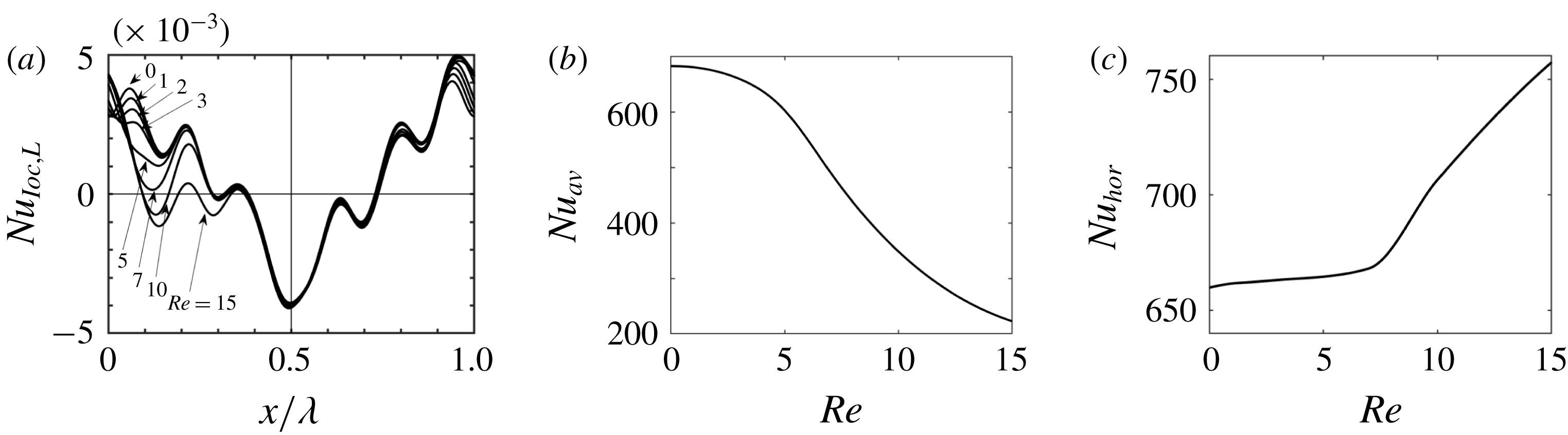
The net heat flux leaving the lower wall and entering the upper wall, which can be expressed in terms of the average Nusselt number $Nu_{av}$ defined as

(4.2) $$\begin{eqnarray}Nu_{av}=\unicode[STIX]{x1D706}^{-1}\int _{0}^{\unicode[STIX]{x1D706}}Nu_{loc,L}\,\text{d}x,\end{eqnarray}$$

provides one measure of energy losses. Its variations with $Re$ illustrated in figure 11(b) demonstrate reduction of this loss as $Re$ increases, in agreement with Hossain & Floryan (Reference Hossain and Floryan2015b ).

Temperature variations along the wall are essential for the creation of convection rolls, and their maintenance leads to another cost. This cost consists of thermal conduction along the wall and heat transfer through the fluid between the hot- and cold-wall segments. The former depends on the wall’s material and structure and, thus, additional assumptions are needed to determine its magnitude. This problem is outside the scope of the present work. The latter can be quantified in terms of the periodic part of the heat flux leaving the wall. Determination of this heat flux, which we shall refer to as the horizontal heat flux, is complicated as its local direction depends on the Reynolds number (see figure 11 a). Its magnitude can be measured using the horizontal Nusselt number ( $Nu_{hor}$ ) defined as

(4.3) $$\begin{eqnarray}Nu_{hor}=\int _{L}\left[-\frac{\unicode[STIX]{x2202}\unicode[STIX]{x1D703}}{\unicode[STIX]{x2202}y}+\frac{\text{d}\emptyset ^{(0)}}{\text{d}y}\right]_{y=-1}\,\text{d}x,\end{eqnarray}$$

where $L$ denotes the part of the wall where $Nu_{loc,L}>0$ and $\emptyset ^{(0)}$ stands for mode zero in the numerical representation of the temperature field. Integration over the part of the wall where $Nu_{loc,L}<0$ produces the same results but with an opposite sign. Results displayed in figure 11(c) demonstrate that the ‘horizontal heat losses’ are always significant; they are nearly constant for $Re<3$ but begin to increase when $Re\gtrsim 7$ .

5 Summary

Analyses of flows in heated horizontal channels were carried out using theoretical and experimental methodologies. A specially designed experimental facility was constructed to realize both well-controlled spatially distributed surface heating and low-Reynolds-number flows with desired flow rates. The theoretical model was generalized to handle experimentally realized heating conditions. The field equations for the Boussinesq fluid were solved with spectral accuracy using Fourier expansions in the streamwise direction and Chebyshev expansions in the wall-normal direction for the heating conditions taken from the experiment.

It was shown that the application of heating in the absence of mean horizontal flow ( $Re=0$ ) results in the formation of convection rolls whose topology is dictated by the heating wavelength. Addition of a mean pressure gradient results in a competition between the buoyancy-driven and the pressure-gradient-driven flows. When $Re$ is very small, this competition results in the formation of a narrow stream tube winding around the convection rolls and separating clockwise-rotating rolls from direct contact with the upper wall and counterclockwise-rotating rolls from direct contact with the lower wall. Increase of $Re$ leads to the dominance of the pressure-gradient-driven effects leading to an increase of the width of this stream tube and eventual elimination of the rolls. The counterclockwise-rotating rolls are eliminated already at $Re\approx 15$ while the clockwise-rotating roll can be identified until $Re\approx 20$ . The change in the flow topology was observed using smoke visualization, PIV measurements as well as theoretical calculations, with the theoretical and experimental results agreeing remarkably well. Velocity measurements provided the means for determination of the wall shear stress. This stress has a spatially periodic distribution with amplitudes two orders of magnitude larger than the isothermal stress. The amplitudes decrease as $Re$ increases but are still very large at $Re=15$ , which is the largest $Re$ used in the experiments. The distributions of shear stresses agree very well with the theoretical predictions.

The theoretical analysis showed that heating leads to a reduction of pressure losses for Reynolds numbers up to $Re\approx 100$ . The largest absolute reduction for the heating conditions used in the experiment is achieved for $Re\approx 14$ while the largest relative reduction with respect to the isothermal conditions is achieved for $Re\approx 11$ . Limitations of the existing instrumentation prevented the direct measurement of the very small pressure drops for the isothermal as well as non-isothermal conditions. The force-balance approach, where the pressure drop can be predicted from the measured shear forces, proved unsuccessful due to the error accumulation in the evaluation of the local shear stress. Accurate measurements of the flow field provide nevertheless indirect verification of the pressure-gradient-reducing effect as the pressure and velocity fields form a closely coupled system.