1 Introduction
Stable density stratification can have a first-order effect on turbulence in the environment, such as in the atmosphere, the oceans, estuaries and lakes. Stable stratification allows for the propagation of internal gravity waves and, when strong, leads to the suppression of vertical motion and the modification of turbulence dynamics. In this paper we report on the impact of strong, stable stratification on initially homogeneous, isotropic turbulence. This allows us to study the effects of stratification on turbulence in one of its simplest forms, without the turbulence being sustained by a source of energy and without the effects of statistical non-homogeneity. The strength of the stratification can be indicated by a local (in time) Froude number,
 $Fr=2\unicode[STIX]{x03C0}U/NL$
, where
 $U$
is an instantaneous root-mean-square (r.m.s.) velocity of the turbulence motions characterised by a length scale
 $L$
, and
 $2\unicode[STIX]{x03C0}/N$
is the buoyancy period. The Froude number, the ratio of the buoyancy time scale
 $2\unicode[STIX]{x03C0}/N$
to the turbulence time scale
 $L/U$
, is expected to decay as the flow decays. Of interest are: how the dynamics of a flow, initiated at a somewhat high Froude number, is modified by the presence of stable stratification; the behaviour of the flow as the stable stratification becomes dominant, i.e. when
 $Fr<O(1)$
, which is estimated to occur at approximately one buoyancy period after flow initiation (Riley, Metcalfe & Weissman Reference Riley, Metcalfe, Weissman and West1981; Liu Reference Liu1995; Spedding Reference Spedding1997); and the subsequent behaviour of the flow as viscous effects become important. We will refer to the flow regime when
 $Fr<O(1)$
as the ‘strongly stratified’ regime.
After the Froude number in a decaying flow has decreased to order one, the nonlinear dynamics is expected to have become significantly altered. For example, the vertical motion along with vortex stretching in the vertical are suppressed (Maffioli & Davidson Reference Maffioli and Davidson2016). In this regime, it is widely thought that the tendency towards the vertical decoupling of horizontal motions and subsequent shearing become an important instability and turbulence-generating mechanism, as suggested by the physical arguments of Lilly (Reference Lilly1983) and the scaling analysis of Billant & Chomaz (Reference Billant and Chomaz2001). These arguments, along with the results from laboratory experiments (e.g. Lin & Pao Reference Lin and Pao1979; Spedding Reference Spedding1997), indicate that in the strongly stratified regime the flow becomes highly anisotropic, and that it is useful to distinguish, for example, the vertical and horizontal integral scales of the r.m.s. horizontal velocity
 $U_{h}$
, i.e.
 $L_{h}$
and
 $L_{v}$
, respectively. The strongly stratified regime will then be defined when
 $Fr_{h}=2\unicode[STIX]{x03C0}U_{h}/NL_{h}$
is small, i.e. when the ratio of the buoyancy period to the horizontal advection time scale
 $L_{h}/U_{h}$
is small. On the other hand, the arguments of Lilly (Reference Lilly1983) and Billant & Chomaz (Reference Billant and Chomaz2001) predict that
 $Fr_{v}=2\unicode[STIX]{x03C0}U_{h}/NL_{v}$
will remain of order 1.
For the most part we narrow our focus to the strongly stratified regime when the Reynolds number
 $Re_{h}=U_{h}L_{h}/\unicode[STIX]{x1D708}$
is large enough so that the buoyancy Reynolds number
 ${\mathcal{R}}=Fr_{h}^{2}Re_{h}$
is greater than order one, although we will also address the regime where
 ${\mathcal{R}}$
is small. Here
 $\unicode[STIX]{x1D708}$
is the kinematic viscosity. The inequality
 ${\mathcal{R}}>O(1)$
implies that the flow is strong enough to continue to cause smaller-scale instabilities and turbulence (Smyth, Klaassen & Peltier Reference Smyth, Klaassen and Peltier1988; Riley & de Bruyn Kops Reference Riley and de Bruyn Kops2003). We will refer to the regime where both
 $Fr<O(1)$
and
 ${\mathcal{R}}>O(1)$
as the ‘stratified turbulence’ regime following Lilly (Reference Lilly1983).
The decay of homogeneous turbulence subject to stable density stratification has been the subject of a number of laboratory experiments, numerical simulations and theoretical analyses. In the laboratory, several studies have been carried out by towing a grid through a salt-stratified water tank (Britter et al. Reference Britter, Hunt, Marsh and Snyder1983; Liu Reference Liu1995; Fincham, Maxworthy & Spedding Reference Fincham, Maxworthy and Spedding1996; Praud, Fincham & Sommeria Reference Praud, Fincham and Sommeria2005), flowing water past a grid in a salt-stratified flume (Stillinger, Helland & Van Atta Reference Stillinger, Helland and Van Atta1983; Itsweire, Helland & Van Atta Reference Itsweire, Helland and Van Atta1986) or flow past a grid in a temperature-stratified wind tunnel (Lienhard & Van Atta Reference Lienhard and Van Atta1990; Yoon & Warhaft Reference Yoon and Warhaft1990). In each case detailed measurements were made downstream of the grid to determine the flow properties and its evolution. These experiments each produced an approximation to homogeneous decay; it must be realised, however, that the laboratory flows are initiated in a somewhat different manner than those in the numerical simulations reported here. In the laboratory experiments the turbulence is generated while the stable stratification is already present, while in our simulations isotropic turbulence is first developed and subsequently the stable stratification is applied.
Considerable insight into the effects of stable stratification on turbulent flows has been gained from these experimental studies. The results for the energy decay rate, however, which is one of the principal motivations of the present study, are mixed. For example, Liu (Reference Liu1995) towed a biplane grid at constant speed in a tank uniformly salt stratified for a range of mesh Froude numbers,
 $Fr_{M}=2\unicode[STIX]{x03C0}U/NM\approx \infty ,80$
and 40; here
 $U$
is the towing speed and
 $M$
the mesh spacing. He found that the kinetic energy decay rate increased from approximately
 $(x/M)^{-1.3}$
for the non-stratified case to
 $(x/M)^{-1.65}$
for the stratified cases. In addition the potential energy decayed as
 $(x/M)^{-1.5}$
, and attained a value of approximately 50 % of the total kinetic energy, indicating that the stratification was playing a significant role in the overall dynamics. Liu also found that the time-local Froude number
 $Fr$
decays as approximately
 $(x/MF_{M})^{-1}$
, as predicted by Riley et al. (Reference Riley, Metcalfe, Weissman and West1981), and became
 $O(1)$
at
 $Nt/2\unicode[STIX]{x03C0}=x/MF_{M}\approx 1$
, indicating the effects of stratification became strong in approximately one buoyancy period. Praud et al. (Reference Praud, Fincham and Sommeria2005) also studied the turbulence behind a towed grid; however, their grid was not biplane, but consisted of the wakes of only vertical plates to eliminate enhanced internal waves which would be generated by horizontal plates. In particular they examined the later time behaviour of the turbulence, where quasi-horizontal motions were observed after the collapse of the three-dimensional turbulence. Remarkably, they observed that the turbulent kinetic energy decay rate was the same as for the non-stratified case. The decay mechanism, however, appeared to be different, as strong vertical shearing developed in the horizontal motions. In wind tunnel experiments, because of the limitations of wind tunnel length, Yoon & Warhaft (Reference Yoon and Warhaft1990) were only able to explore turbulence decay for approximately one buoyancy period. They did find, however, contrary to the results of Liu (Reference Liu1995) and Praud et al. (Reference Praud, Fincham and Sommeria2005), that stable stratification inhibited the turbulence decay. Similarly, in their water channel experiments, Stillinger et al. (Reference Stillinger, Helland and Van Atta1983) also found that stable stratification inhibited the decay of the turbulence. Therefore, from these laboratory experiments, it is unclear whether stable stratification might enhance or inhibit turbulence decay, and what the corresponding mechanisms might be.
The effects of stable stratification on turbulent wake decay were obtained from the laboratory experiments of Lin & Pao (Reference Lin and Pao1979) and Spedding (Reference Spedding1997) conducted in the wake of a slender, axisymmetric body and of a sphere, respectively. In both cases the model was towed at constant speed through a uniformly stratified water tank. The experiments of Lin & Pao (Reference Lin and Pao1979) were carried out in a Reynolds number range of
 $2\times 10^{4}\leqslant Re_{D}\leqslant 3\times 10^{4}$
and a Froude number range of
 $23\leqslant F_{D}\leqslant 120$
, where
 $Re_{D}=UD/\unicode[STIX]{x1D708}$
and
 $F_{D}=2\unicode[STIX]{x03C0}U/ND$
;
 $U$
and
 $D$
are the towing speed and the diameter defined from projected area of the model, respectively. It might be expected that the wake of a slender object or a sphere would decay faster for experiments with stable stratification than for ones without stratification, since internal wave radiation (Watanabe et al.
Reference Watanabe, Riley, de Bruyn Kops, Diamessis and Zhou2016) would lead to additional decrease in the energy in the wake region. Lin & Pao (Reference Lin and Pao1979) found, for example, that the turbulence behaviour for stratified cases was about the same as for non-stratified cases up to approximately one to two buoyancy periods after the initiation of the turbulence. At that point, however, the turbulence in the streamwise direction began to decay more slowly, while that in the vertical direction decayed faster. Spedding (Reference Spedding1997) performed experiments for Reynolds numbers in the range
 $1.0\times 10^{4}\leqslant Re_{D}\leqslant 2.3\times 10^{4}$
, and Froude numbers in the range
 $31.4\leqslant F_{D}\leqslant 753$
, where now the Froude number is defined as
 $F_{D}=U/ND$
. In a similar vein, Spedding found that at approximately one third of a buoyancy period downstream from the sphere, the decay rate of the centreline mean velocity decreased from the non-stratified rate of
 $(Nt)^{-2/3}$
to
 $(Nt)^{-1/4}$
. The regime with the slow decay rate he referred to as the non-equilibrium regime. Furthermore he found that, at approximately ten buoyancy periods, the decay rate increased to approximately
 $(Nt)^{-3/4}$
. He referred to this as the quasi-two-dimensional regime, where a quasi-horizontal vortex wake, but with variation in the vertical, was clearly apparent in visualisations, as also seen in previous experiments (Lin & Pao Reference Lin and Pao1979).
Godoy-Diana, Chomaz & Billant (Reference Godoy-Diana, Chomaz and Billant2004) performed a laboratory study meant to simulate ‘pancake’ vortices similar to what is seen in the quasi-horizontal wakes of Lin & Pao (Reference Lin and Pao1979) and Spedding (Reference Spedding1997). A vertically uniform vortex pair is generated with vertical flaps in a salt-water stratified tank. The generated vortices were allowed to pass through a horizontal slot, narrowing their vertical range. Godoy-Diana et al. (Reference Godoy-Diana, Chomaz and Billant2004) found two regimes for the time dependence of the vertical scale
 $L_{v}$
of the vortices; in both cases the value of
 ${\mathcal{R}}$
was fairly small. In particular, they found for one of their cases that
 $L_{v}=L_{h}Re_{h}^{-1/2}$
, similar to the results of Maffioli & Davidson (Reference Maffioli and Davidson2016) when
 ${\mathcal{R}}$
was small. They discussed these results in terms of the scaling analysis introduced by Riley et al. (Reference Riley, Metcalfe, Weissman and West1981), but with the effect of viscosity included. These results will be discussed further in § 3.2.
Many numerical simulations have been conducted to understand decaying stratified turbulence, beginning with the work of Riley et al. (Reference Riley, Metcalfe, Weissman and West1981). They initiated their simulations by allowing the turbulence to develop nonlinearly without stratification, and then applying the density stratification. They found that stratification introduced a wave-like character in the flow field, with exchanges of kinetic and potential energies and the development of counter-gradient buoyancy fluxes, something also observed in the laboratory by Liu (Reference Liu1995). Contrary to some of the laboratory experiments mentioned, but qualitatively consistent with others, they found that the stable stratification slightly inhibited the total energy decay rate. They found that stratification modified the nonlinear dynamics by inhibiting vortex stretching and suppressing the vertical component of the kinetic energy. Finally they introduced scaling arguments to explain the quasi-horizontal motions observed in the laboratory data.
A number of other simulations of homogeneous, stably stratified turbulence have been performed, using different initial conditions and for different research purposes. For example Herring & Métais (Reference Herring and Métais1989), and Métais & Herring (Reference Métais and Herring1989) initiated or forced their flows with vertically independent, horizontal motions, but with very small amplitude, three-dimensional noise added, in order to study the effects of stable density stratification on the three-dimensional breakdown of the flows. They found the two-dimensional motions collapsed into thin horizontal layers, which had been suggested by the heuristic arguments of Lilly (Reference Lilly1983) and was later predicted by the scaling analysis of Billant & Chomaz (Reference Billant and Chomaz2001).
With the introduction of larger computers, various initial conditions have been used to understand particular aspects of the strongly stratified flow regime. For example, Riley & de Bruyn Kops (Reference Riley and de Bruyn Kops2003) considered an initial Taylor–Green configuration, conceived of as an idealisation of the quasi-two-dimensional regime downstream of a grid or a sphere. Although the simulations were initialised with overall Richardson numbers well above one, they found that the Richardson numbers sharply decreased in time until the flows became unstable due to the vertical shearing of the horizontal motions, as suggested by Lilly (Reference Lilly1983). They also observed a
 $-5/3$
behaviour of the horizontal wavenumber spectrum, something ultimately predicted by Lindborg (Reference Lindborg2006). In contrast, Bartello & Tobias (Reference Bartello and Tobias2013) examined decaying homogeneous turbulence but starting with isotropic, random-phase velocity fields. They found results consistent with the scaling arguments of Lindborg (Reference Lindborg2006) as long as the buoyancy Reynolds number
 ${\mathcal{R}}$
was high enough. Maffioli & Davidson (Reference Maffioli and Davidson2016) employed a similar initialisation to study the decay of homogeneous, stratified turbulence. They introduced a scaling analysis of the vorticity equation, emphasising the importance of the vertical shearing of the horizontal motion, as argued by Lilly (Reference Lilly1983) and Billant & Chomaz (Reference Billant and Chomaz2001). They found that the dissipation scaling
 $\unicode[STIX]{x1D716}\sim U_{h}^{3}/L_{h}$
was valid for the entire range of
 ${\mathcal{R}}$
, and also found agreement with the
 $-5/3$
horizontal spectral range, as argued by Lindborg (Reference Lindborg2006). Finally, they found that, once the effects of stratification became strong, then
 $Fr_{v}$
remained approximately a constant of order 1. Brethouwer et al. (Reference Brethouwer, Billant, Lindborg and Chomaz2007) considered forced, strongly stratified turbulence for a range of Froude and Reynolds numbers. They found two regimes depending on the value of
 ${\mathcal{R}}$
. For large
 ${\mathcal{R}}$
,
 $L_{v}\sim U_{h}/N$
, i.e.
 $Fr_{v}\sim 1$
. For small
 ${\mathcal{R}}$
, however, they found that
 $L_{v}\sim L_{h}/Re_{h}^{1/2}$
. Furthermore they found horizontal wavenumber spectra somewhat consistent with the predictions of Lindborg (Reference Lindborg2006).
Using fully nonlinear numerical simulations, Diamessis, Spedding & Domaradzki (Reference Diamessis, Spedding and Domaradzki2011) simulated the experiments of Spedding (Reference Spedding1997) for the wake of a sphere for a range of Reynolds numbers. In particular they found that the temporal extent of the non-equilibrium regime defined by Spedding increased as the Reynolds number increased. This prolongation was found to be due to instabilities in inclined shear layers, whose thicknesses decreased as the Reynolds number increased.
Davidson (Reference Davidson2010) addressed the issue of the decay of homogeneous, strongly stratified turbulence (
 $Fr<O(1)$
) using the theoretical approach of Saffman (Reference Saffman1967). Studying the decay of homogeneous, isotopic turbulence, Saffman (Reference Saffman1967) assumed that the kinetic energy spectrum behaves as
 $E(k)\sim k^{2}$
as
 $k\rightarrow 0$
, and predicted that
 $$\begin{eqnarray}U^{2}\sim t^{-6/5},\quad L\sim t^{2/5},\end{eqnarray}$$
where
 $U$
is the instantaneous r.m.s. velocity of the turbulence motions with integral length scale
 $L$
. Following Saffman’s approach, Davidson (Reference Davidson2010) was able to establish that, for homogeneous, strongly stratified turbulence,
 $U_{h}^{2}L_{h}^{2}L_{v}\approx \text{const}$
. Here
 $U_{h}$
and
 $L_{h}$
are characteristic horizontal r.m.s. velocity and horizontal integral scales, respectively, and
 $L_{v}$
is a characteristic vertical integral scale. Then, using the additional constraint
 $U_{h}/NL_{v}\sim 1$
(Billant & Chomaz Reference Billant and Chomaz2001) and the observation that
 $\unicode[STIX]{x1D716}\sim U_{h}^{3}/L_{h}$
, he predicted that
 $$\begin{eqnarray}U_{h}^{2}\sim t^{-4/5},\quad L_{h}\sim t^{3/5},\quad L_{v}\sim t^{-2/5}.\end{eqnarray}$$
Therefore Davidson predicted a slower decay of the horizontal r.m.s. velocity due to stable stratification. On the other hand he predicted a faster growth of the horizontal integral scale of the horizontal r.m.s. velocity, but a decay with time of the vertical integral scale of the horizontal r.m.s. velocity.
In the next section the numerical approach to the simulations will be outlined, followed by our simulation results in § 3. In that section we will discuss, in particular, the effects of stratification on the decay characteristics of the flow, on the flow energetics, on the dissipation rates and mixing efficiency and on energy spectra. We will also address the modification of these results as the effects of viscosity become important. Finally, in § 4 we will further discuss our results and present our conclusions.
2 Numerical methodology
In the introduction, we narrowed our scope of interest to flows with initially high Froude number that decay until
 $Fr<O(1)$
but with
 ${\mathcal{R}}=Fr_{h}^{2}Re_{h}$
high enough to sustain turbulence. To study such flows we consider three decaying stratified flow simulations which differ only in Reynolds number so that each transitions through about the same range of Froude numbers but with differing values of
 ${\mathcal{R}}$
. Corresponding to each stratified case is a non-stratified simulation initialised with exactly the same fields. So six simulations are used for this study but, since the non-stratified cases are used only to provide reference for the stratified cases, we refer to the simulations in terms of three cases, each with a stratified and non-stratified simulation.
To create the initial velocity fields, simulations with no stratification are forced to match Pope’s model spectrum with his parameters
 $p_{0}=2$
and
 $c_{L}=6.78$
(Pope Reference Pope2000, equation 6.247). This is accomplished by applying a deterministic forcing schema similar to that of Overholt & Pope (Reference Overholt and Pope1998) (cf. Rao & de Bruyn Kops Reference Rao and de Bruyn Kops2011). For this initialisation process, the methodology is the same as that discussed in Almalkie & de Bruyn Kops (Reference Almalkie and de Bruyn Kops2012a
). In short, a pseudospectral method is used to solve the discretised Navier–Stokes equations. The advection term in the momentum equation is solved in rotation form. When scalar transport is included, the advection term solved in conservation and convection forms on alternating time steps to approximate the skew-symmetric form and ensure energy conservation. The third-order Adams–Bashforth method with pressure projection is used to advance the equations in time, as suggested by Durran (Reference Durran1991). The fields are fully dealiased using the
 $2/3$
-method of truncation.
The forcing schema involves solving overdamped, second-order ordinary differential equations for the kinetic energy in each wavenumber shell in order to converge the simulated spectrum to a target spectrum. Since the forcing responds to the evolving flow field, convergence is achieved in the quasi-stationary sense. Once statistical stationarity is observed, forcing is turned off and the flow is allowed to relax, still with zero buoyancy force, until power-law decay is observed. The virtual origin for power-law decay is designated
 $\hat{t}_{0}$
. Next we define the dimensionless time
 $t\equiv (\hat{t}-\hat{t}_{0})/\hat{t}_{LE}=1$
as the starting point for the simulations. Here, time is non-dimensionalised by the large-eddy advective time scale
 $\hat{t}_{LE}=\hat{L}/\hat{U}$
with
 $\hat{L}$
the integral length scale of the turbulence at
 $t=1$
and
 $\hat{U}$
the corresponding r.m.s. velocity. The initial velocity fields for the stratified simulations, and for the corresponding non-stratified flow simulations, are those at
 $t=1$
.
Note that while the initialisation of the three simulation cases started by forcing them all to the same target spectrum, the velocity fields are different locally and the Reynolds numbers are different; so the simulations decay at different rates and have slightly different virtual origins. In order to easily compare the three cases, we have introduced the notation
 $\hat{(~)}$
to denote a dimensional quantity. Since this notation can be cumbersome to read, it was not used in § 1.
There are two time scales of interest in decaying stratified flows. One is the advective time scale, which in dimensional terms is
 $\hat{t}_{LE}=\hat{L}/\hat{U}$
. The second time scale is the buoyancy period, which in dimensional terms is
 $\hat{T}_{B}=2\unicode[STIX]{x03C0}/\hat{N}$
. It is usual to examine the flow variables as functions of
 $t$
, i.e. time scaled by the advective time
 $\hat{t}_{LE}$
. It is sometimes useful, however, to observe the flows in terms of the number of buoyancy periods after stratification has been applied, that is, in terms of
 $T$
defined by
 $$\begin{eqnarray}T=\left.\left(\hat{t}-\hat{t}_{0}-\frac{\hat{L}}{\hat{U} }\right)\right/\hat{T}_{B}=\frac{t-1}{Fr}.\end{eqnarray}$$
Both times will be used in presenting our results.
To impose stratification at
 $t=1$
, two changes are made to the simulations. First, a uniform, time-invariant, stable ambient density gradient with magnitude
 $\text{d}\overline{\hat{\unicode[STIX]{x1D70C}}}/\text{d}\hat{z}$
is applied. Note that, from this density gradient, a density scale can be defined by
 $\hat{\unicode[STIX]{x1D70C}}=\hat{L}\text{d}\overline{\hat{\unicode[STIX]{x1D70C}}}/\text{d}\hat{z}$
. Second, the governing equations being solved are modified to satisfy the non-hydrostatic Boussinesq assumption. Thus, after density stratification has been applied, the dimensionless governing equations are:
 $$\begin{eqnarray}\displaystyle & \displaystyle \frac{\unicode[STIX]{x2202}\boldsymbol{v}}{\unicode[STIX]{x2202}t}+\boldsymbol{v}\boldsymbol{\cdot }\unicode[STIX]{x1D6FB}\boldsymbol{v}=-\left(\frac{2\unicode[STIX]{x03C0}}{Fr}\right)^{2}\unicode[STIX]{x1D70C}\boldsymbol{e}_{z}-\unicode[STIX]{x1D735}p+\frac{1}{Re}\unicode[STIX]{x1D6FB}^{2}\boldsymbol{v}, & \displaystyle\end{eqnarray}$$
 $$\begin{eqnarray}\displaystyle & \displaystyle \unicode[STIX]{x1D735}\boldsymbol{\cdot }\boldsymbol{v}=0, & \displaystyle\end{eqnarray}$$
 $$\begin{eqnarray}\displaystyle & \displaystyle \frac{\unicode[STIX]{x2202}\unicode[STIX]{x1D70C}}{\unicode[STIX]{x2202}t}+\boldsymbol{v}\boldsymbol{\cdot }\unicode[STIX]{x1D735}\unicode[STIX]{x1D70C}-w=\frac{1}{RePr}\unicode[STIX]{x1D6FB}^{2}\unicode[STIX]{x1D70C}. & \displaystyle\end{eqnarray}$$
 $\boldsymbol{v}=(u,v,w)$
is the velocity vector in the Cartesian coordinate system
 $\boldsymbol{x}=(x,y,z)$
with
 $z$
oriented in the vertical direction,
 $\unicode[STIX]{x1D70C}$
and
 $p$
are the density and pressure deviations from their ambient values and
 $Pr=\hat{\unicode[STIX]{x1D708}}/\hat{D}$
is the Prandtl number, which is taken to be unity;
 $\hat{\unicode[STIX]{x1D708}}$
is the kinematic viscosity and
 $\hat{D}$
the density diffusivity. The equations have been non-dimensionalised by the length scale
 $\hat{L}$
, the time scale
 $\hat{t}_{LE}$
and the density scale
 $\hat{\unicode[STIX]{x1D70C}}$
defined above. In the present simulations,
 $\hat{L}$
is taken to be
 $\hat{L}_{h}$
, the longitudinal integral scale in the horizontal direction at
 $t=1$
. The nominal Reynolds number
 $Re$
, Froude number
 $Fr$
, and time scaling are defined by the flow conditions at the instant stratification is applied (
 $t=1$
) as
 $$\begin{eqnarray}Re=\frac{\hat{U} \hat{L}}{\hat{\unicode[STIX]{x1D708}}},\quad Fr=\frac{2\unicode[STIX]{x03C0}\hat{U} }{\hat{N}\hat{L}},\quad t=\frac{\hat{t}-\hat{t}_{0}}{\hat{t}_{LE}},\end{eqnarray}$$
where
 $\hat{N}=[-({\hat{g}}/\hat{\unicode[STIX]{x1D70C}}_{0})/(\text{d}\overline{\hat{\unicode[STIX]{x1D70C}}}/\text{d}\hat{z})]^{1/2}$
is the buoyancy frequency,
 ${\hat{g}}$
is the gravitational acceleration in the
 $-z$
direction and
 $\hat{\unicode[STIX]{x1D70C}}_{0}$
is the density at a reference elevation
 $\hat{z}_{0}$
. In terms of dimensionless quantities, the total density is
 $$\begin{eqnarray}\unicode[STIX]{x1D70C}_{t}=\unicode[STIX]{x1D70C}_{0}+(z-z_{0})+\unicode[STIX]{x1D70C}.\end{eqnarray}$$
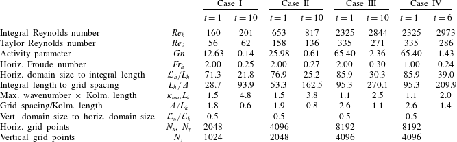
Parameters for the three stratified flow simulations considered are listed in table 1. The only difference in input parameters between the simulations is the Reynolds number and, hence, there are different requirements on the small-scale numerical resolution for each simulation. The integral Reynolds number
 $Re_{h}$
and Froude number
 $Fr_{h}$
are defined in terms of the r.m.s. horizontal velocity and horizontal velocity longitudinal integral scale. The initial Froude number for each case is 2.0, and the initial Reynolds numbers are 160 (Case I), 653 (Case II) and 2325 (Case III). The Reynolds number for laboratory data is often given in terms of the Reynolds number based upon the Taylor microscale,
 $Re_{\unicode[STIX]{x1D706}}$
. The initial values of
 $Re_{\unicode[STIX]{x1D706}}$
for the simulations are 56 (Case I), 158 (Case II) and 335 (Case III). These can be compared to 160, the highest value in the experiments of Praud et al. (Reference Praud, Fincham and Sommeria2005).
Simulation parameters and metrics at two times for each stratified simulation. There is a corresponding unstratified simulation with identical conditions at
 $t=1$
. ‘Integral length’ is the average of the two horizontal longitudinal integral length scales each computed as recommended in appendix E of Comte-Bellot & Corrsin (Reference Comte-Bellot and Corrsin1971).

The resolution of the simulations was chosen to enable simulating for long times (over more than 100 buoyancy periods) while satisfying the small-scale and large-scale resolution requirements identified by Eswaran & Pope (Reference Eswaran and Pope1988) and de Bruyn Kops & Riley (Reference de Bruyn Kops and Riley1998), respectively. In particular, the domain is at least 20 times the horizontal integral length scale, even at late times, and the maximum wavenumber, after application of the dealiasing filter, times the Kolmogorov length scale is at least unity at early times. Note that the grid spacing
 $\unicode[STIX]{x1D6E5}$
is the effective size after dealiasing. Finally, note that an additional case, Case IV, was computed with the same initial velocity field as for Case III, but at a different initial Froude number of 1.0. This case was simulated in order to explore the dependence of the results on the initial Froude number, and its results are discussed in § 4 which gives the conclusions and discussion.
3 Simulation results
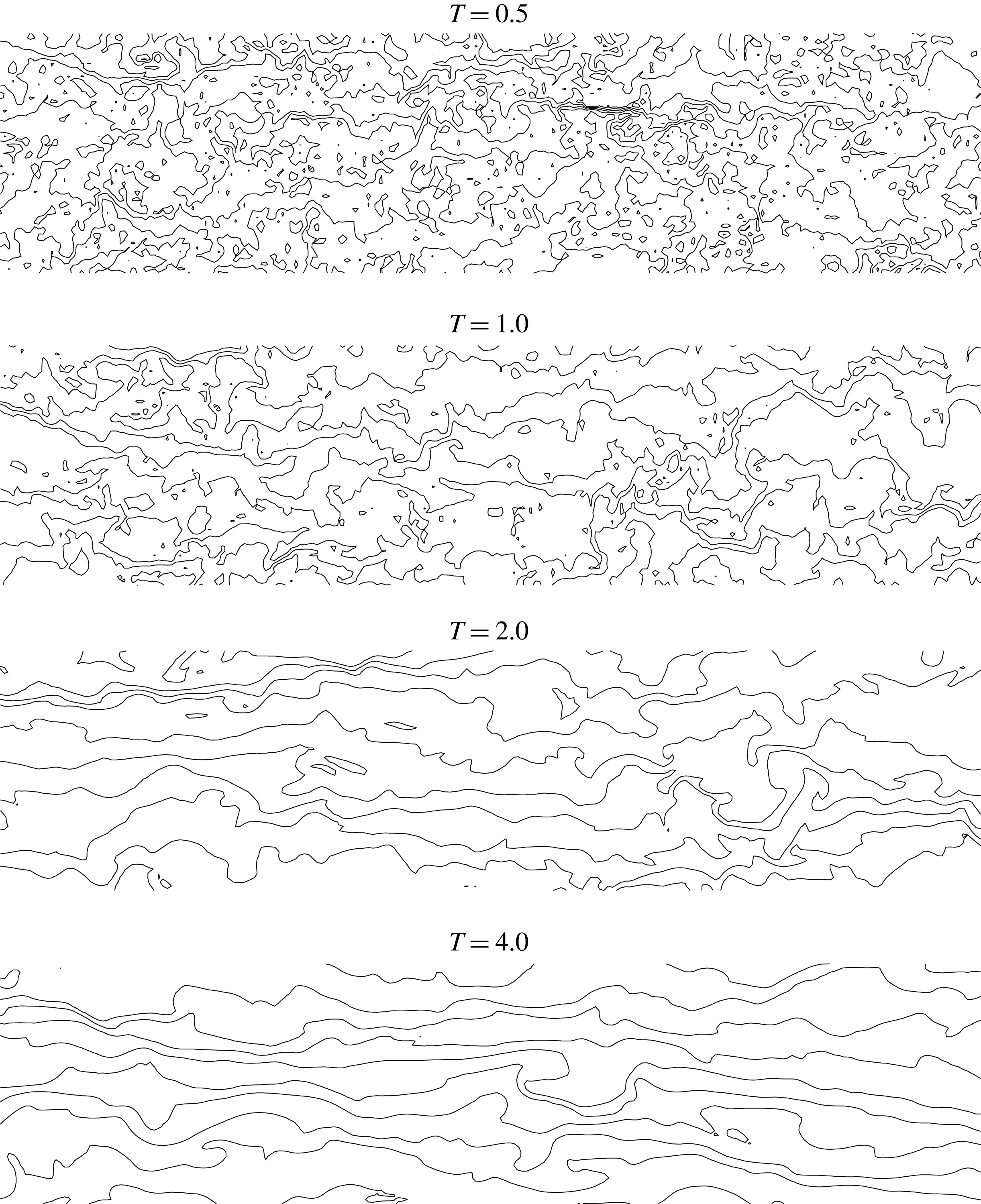
Some qualitative idea of the behaviour of the stratified flows as they decay can be seen in figure 1, which gives lines of constant total density on a vertical plane at several different early times for Case III. For ease of visualisation, only shown is a section of a vertical plane consisting of the upper
 $1/32$
and the leftmost
 $1/16$
of the computational grid. Of course initially the lines are horizontal, as the initial density fluctuations are 0. Early on in the simulation, at
 $T=0.5$
, where time here is measured in buoyancy periods, the lines become highly contorted, with considerable density overturning, much as would be the case for a flow without gravity. As the flow evolves, however, the lines become more horizontal and, by
 $T=4.0$
, only a few regions of overturning are evident. The effects of stably stratification on the flow are clearly evident.
Lines of constant total density on a vertical plane at several times for Case III. The upper
 $1/32$
and the leftmost
 $1/16$
of the domain is plotted.

3.1 Early and intermediate time results
We first address the early and intermediate time development of the stratified flows, defined here as when the effects of viscosity play only a secondary role in the development of the flows. We will find later (see § 3.2 below) that this flow regime extends to approximately 2 buoyancy periods for Case I, 4 buoyancy periods for Case II and approximately 11 buoyancy periods for Case III.
3.1.1 Power-law scaling and the virtual origins
We begin by examining the decay of non-stratified homogeneous, isotropic turbulence for the three cases used as the initial conditions for the stratified cases, and refer the reader to George (Reference George1992), Skrbek & Stalp (Reference Skrbek and Stalp2000) and Davidson (Reference Davidson2010), and the references therein, for theoretical and experimental studies of the decay of homogeneous, isotropic turbulence. A primary interest here is in the power-law decay relationships
 $$\begin{eqnarray}\left.\begin{array}{@{}c@{}}\displaystyle u^{\prime }\propto t^{-n},\\ \displaystyle L^{\prime }\propto t^{m},\end{array}\right\}\end{eqnarray}$$
where
 $u^{\prime }$
is the volume-averaged r.m.s. value of any of the velocity components,
 $t$
is measured from a virtual origin
 $t_{0}$
and
 $L^{\prime }$
is the corresponding integral length scale, either longitudinal or transverse. If
 $L^{\prime }$
is proportional to
 ${u^{\prime }}^{3}/\unicode[STIX]{x1D716}$
, where
 $\unicode[STIX]{x1D716}$
is the volume-averaged dissipation rate of turbulence kinetic energy, then
 $m=1-n$
, although with laboratory or numerical simulation data for homogeneous, isotropic turbulence this relationship may not be observed exactly and many studies report only
 $n$
(cf. de Bruyn Kops & Riley Reference de Bruyn Kops and Riley2000). From the plots by Perot & de Bruyn Kops (Reference Perot and de Bruyn Kops2006) of
 $n$
as a function of Reynolds number based on data from numerous sources, and from Saffman’s theory (Saffman Reference Saffman1967; Davidson Reference Davidson2010), we expect
 $n\approx 0.6$
for the current simulations.
The interdependence of
 $n$
and the virtual origin
 $t_{0}$
makes the calculation of these parameters and their corresponding uncertainties dependent on how the curve fitting is carried out, which is beyond the scope of this paper. Here our immediate objective is to establish that the non-stratified simulations exhibit power-law decay with a value of
 $n$
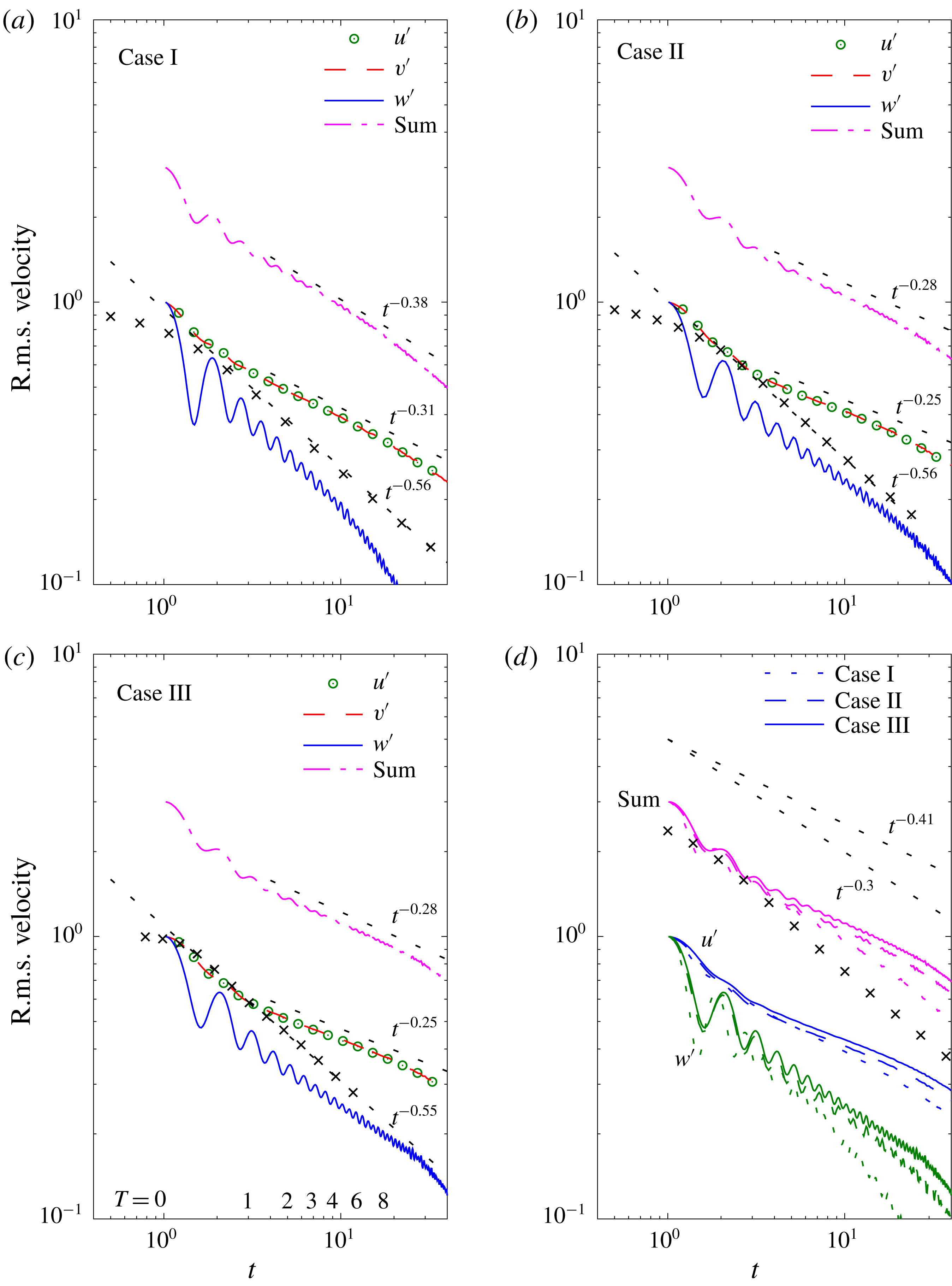
consistent with that in the literature. Figure 2 indicates that this is the case. In the plots
 $u^{\prime }$
,
 $v^{\prime }$
and
 $w^{\prime }$
denote the r.m.s. velocities in the
 $x$
,
 $y$
and
 $z$
directions, respectively, with
 $z$
in the vertical direction. In the figure, the symbols representing the non-stratified flow data lie on curves corresponding to
 $n=0.56$
, 0.56 and 0.55 for Reynolds numbers 160 (Case I), 600 (Case II) and 2325 (Case III), respectively. These are consistent with the expectation that
 $n\approx 0.6$
.
Root-mean-square velocities versus time
 $t$
. Symbols are for non-stratified cases (only for Case I in d). The reference slopes are determined by least-squares fits to the logarithms of the data in the adjacent lines or symbols.

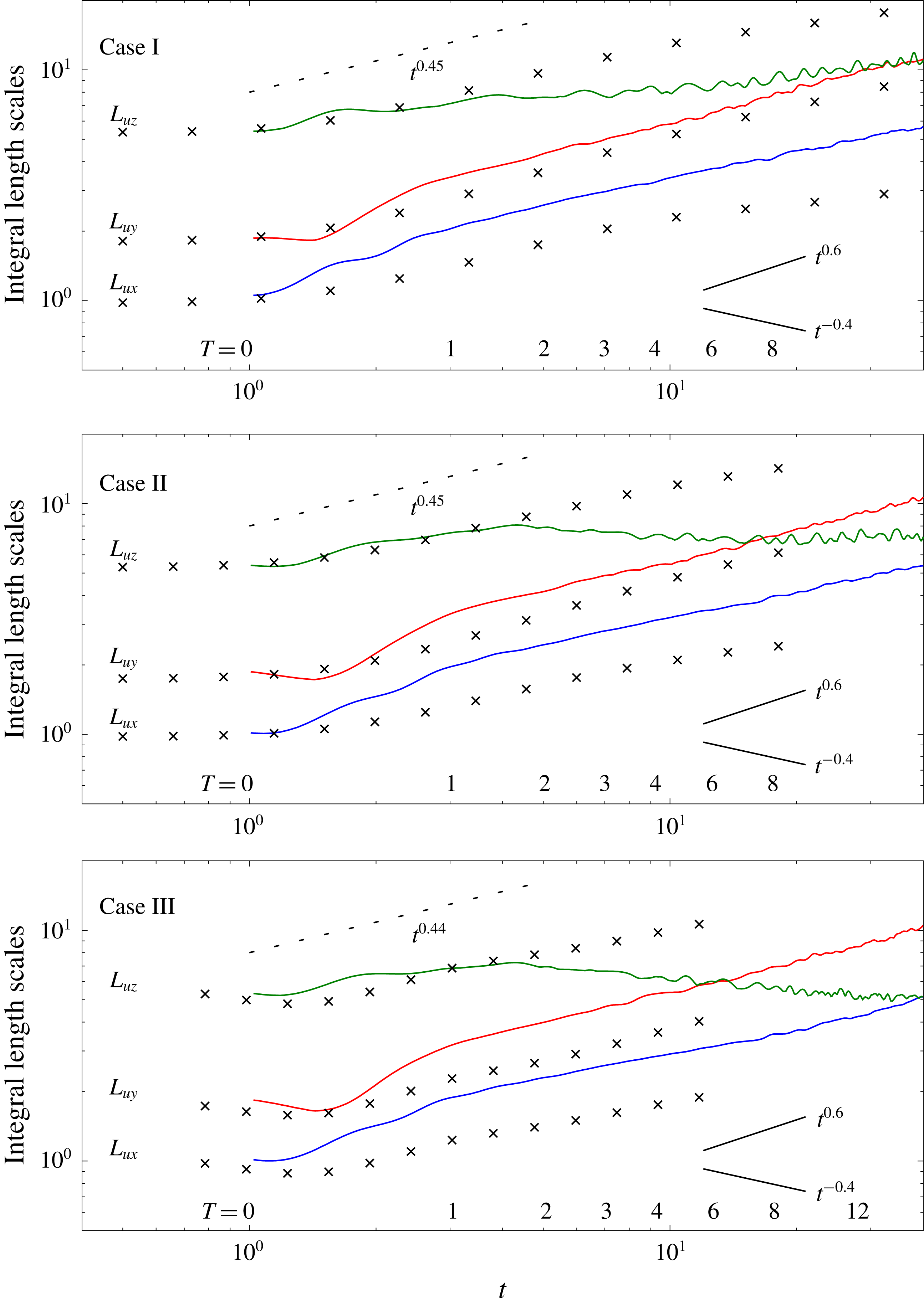
The longitudinal and transverse integral lengths of
 $u$
versus time. The longitudinal scales
 $L_{ux}$
are plotted true and the others are offset vertically in increments of half-decades. The symbols are for non-stratified cases. The dashed-line reference slopes are
 $1-n$
from the non-stratified simulations. The solid-line reference slopes are as derived in Davidson (Reference Davidson2010).

3.1.2 Power-law scaling in the stratified flows
Also plotted in figure 2 are the r.m.s. velocities and in figure 3 the integral length scales for the three stratified cases, the latter which are computed as recommended in appendix E of Comte-Bellot & Corrsin (Reference Comte-Bellot and Corrsin1971). The notation
 $L_{ux}$
denotes the integral length scale of
 $u$
in the
 $x$
-direction, defined in terms of the autocorrelation of
 $u$
, and similarly for the other length scales.
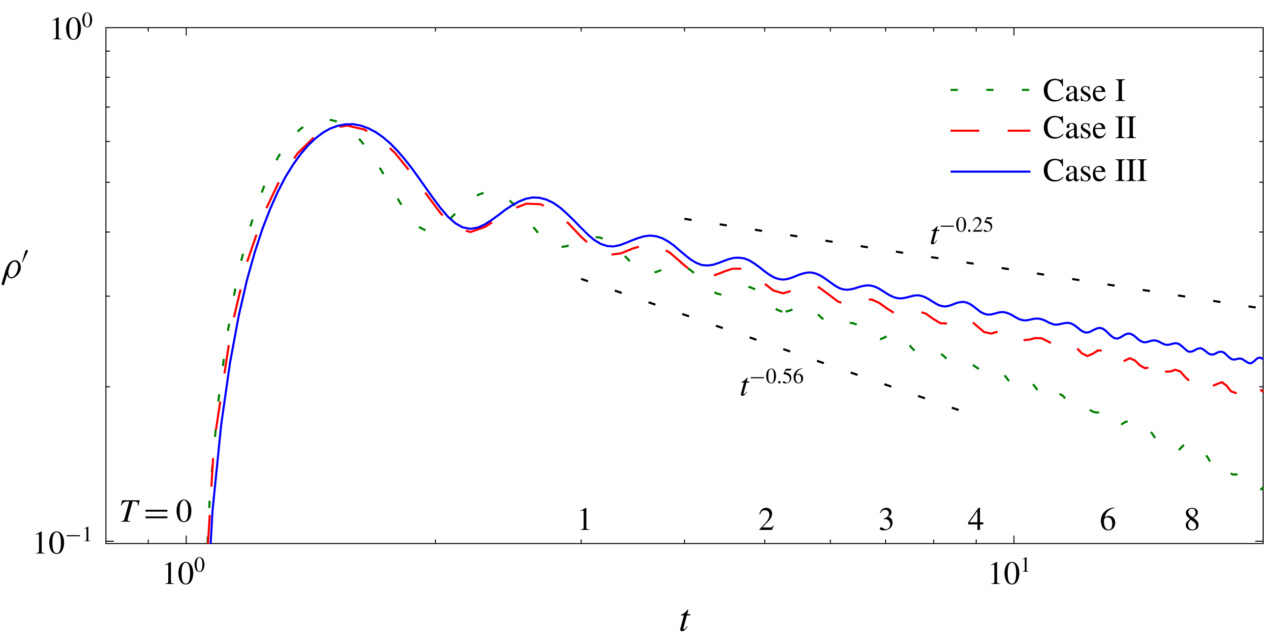
Consider first the r.m.s. velocities, which are plotted in figure 2. There is an adjustment immediately following the onset of stratification at
 $t=1$
, the abruptness of which can be observed in the evolution of the r.m.s. density in figure 4. By approximately
 $t=3$
(
 $T=1$
, i.e. one buoyancy period), the decay rates for
 $u^{\prime }$
and
 $v^{\prime }$
begin to deviate from their non-stratified values, and settle into power-law decay rates which are less than the non-stratified values; they are:
 $n=0.31$
for Case I, and
 $n=0.25$
for Cases II and III. From these results, and from figure 2(d), it is seen that the decay rates are very weakly dependent on the Reynolds number, with the fastest decay rate observed for Case I, the case with the lowest Reynolds number. This observed decrease in the decay rate due to stable stratification is consistent with the prediction of Davidson (Reference Davidson2010), although the decay rates are slightly less (in absolute value) than his estimate of
 $t^{-0.4}$
. The reduction in decay rate is also qualitatively consistent with the experiments of Lin & Pao (Reference Lin and Pao1979), Stillinger et al. (Reference Stillinger, Helland and Van Atta1983), Yoon & Warhaft (Reference Yoon and Warhaft1990) and Spedding (Reference Spedding1997), and with the observations of Almalkie & de Bruyn Kops (Reference Almalkie and de Bruyn Kops2012b
) who, in simulations forced to maintain constant energy in a narrow band of small wavenumbers, observed that stronger stratification slightly reduces the dissipation rate. These results are inconsistent with the laboratory experiments of Liu (Reference Liu1995), however, who finds a decay rate of the horizontal velocities of approximately
 $n=0.825$
with stratification, faster than the rate of 0.65 for his non-stratified case. They are also inconsistent with the results of Praud et al. (Reference Praud, Fincham and Sommeria2005) who found the decay rate of approximately
 $n=0.65$
for all their non-stratified and stratified cases. Note that, in our simulations with stable stratification, after some initial adjustment,
 $w^{\prime }$
decays at almost the same rate as with no stratification for cases II and III. When the Reynolds number is low (Case I at later times) however,
 $w^{\prime }$
decays faster with stratification than without. This is most easily observed in figure 2(a).
Root-mean-square of the fluctuating density
 $\unicode[STIX]{x1D70C}^{\prime }$
versus time
 $t$
. The dashed reference slopes are from the total r.m.s. velocities in the stratified cases.

In figure 3 it is seen that the growth rates of all the horizontal integral length scales are enhanced by the density stratification. The growths of the vertical integral scales of
 $u^{\prime }$
, however, are so strongly affected by the stratification as to become negative at later times for cases Case II and Case III. Both of these results are qualitatively consistent with the predictions of Davidson (Reference Davidson2010). The result for the vertical scales is consistent with the suggestion by Lilly (Reference Lilly1983) that, as the effects of stratification become important, the vertical shearing of the horizontal velocities increases. It is also consistent with the scaling analysis of Billant & Chomaz (Reference Billant and Chomaz2001). The fact that all but the vertical lengths are larger in the stratified cases than in the non-stratified cases does not necessarily mean that coherent structures are larger, but rather that the small scales are suppressed. This will become more apparent when we discuss energy spectra.
The r.m.s. of the density fluctuations provides yet another measure of the decay rate of turbulence with stable density stratification. For a passive scalar
 $\unicode[STIX]{x1D719}$
in isotropic turbulence with
 $u^{\prime }\propto t^{-n}$
, similarity analysis and data indicate that
 $\unicode[STIX]{x1D719}^{\prime }\propto t^{-n}$
as well (cf. de Bruyn Kops & Riley Reference de Bruyn Kops and Riley2000). Since the stratified flows exhibit different decay rates for the horizontal and vertical velocities, we might not expect the decay rate of the scalar fluctuations to agree with that of any single velocity component. From figure 4, however, it is observed that for cases II and III the decay rate of the density fluctuations is almost the same as that of the total r.m.s. velocity. Interpreting
 ${\unicode[STIX]{x1D70C}^{\prime }}^{2}$
in terms of potential energy (see § 3.1.3), this implies that the potential energy decays at almost the same rate as the horizontal components of the kinetic energy for these cases. Significant Reynolds number effects are observed in the figure. For the case with lowest Reynolds number, the decay rate of the scalar after
 $T=1$
is faster than for the total r.m.s. velocity. At later times in this case (Case I), the decay rate is even faster than for the non-stratified simulation, consistent with it following decay rate of
 $w^{\prime }$
. Recall, for example, that Liu (Reference Liu1995) observed that stratification increased the decay rate of velocity, especially the vertical velocity, and so Case I at later times may provide some insight into the dynamics of those laboratory experiments. This issue will be addressed further in § 3.2.
Noticeable in the plots of
 $w$
and
 $\unicode[STIX]{x1D70C}$
is oscillatory behaviour, indicating a wave-like behaviour for these flows. The period of oscillation is approximately
 $0.4\,T_{B}$
for Case I, and appears to lengthen slightly with Reynolds number. The early time dynamics of these flows is strongly nonlinear, however, so that one would not expect internal waves with distinct dispersion relationships to exist at early times. Note that the Froude number
 $Fr_{h}$
can be considered as an estimate of the nonlinear term compared to the time derivative term in the momentum equation. Therefore, as the flows evolve and
 $Fr_{h}$
drops below order 1, one would expect internal waves to exist in the flows, but strongly modified by other motions in the flows. It is possible that the reduced decay rates in the flows is partially due to the appearance of internal wave-like motions.
3.1.3 Flow energetics
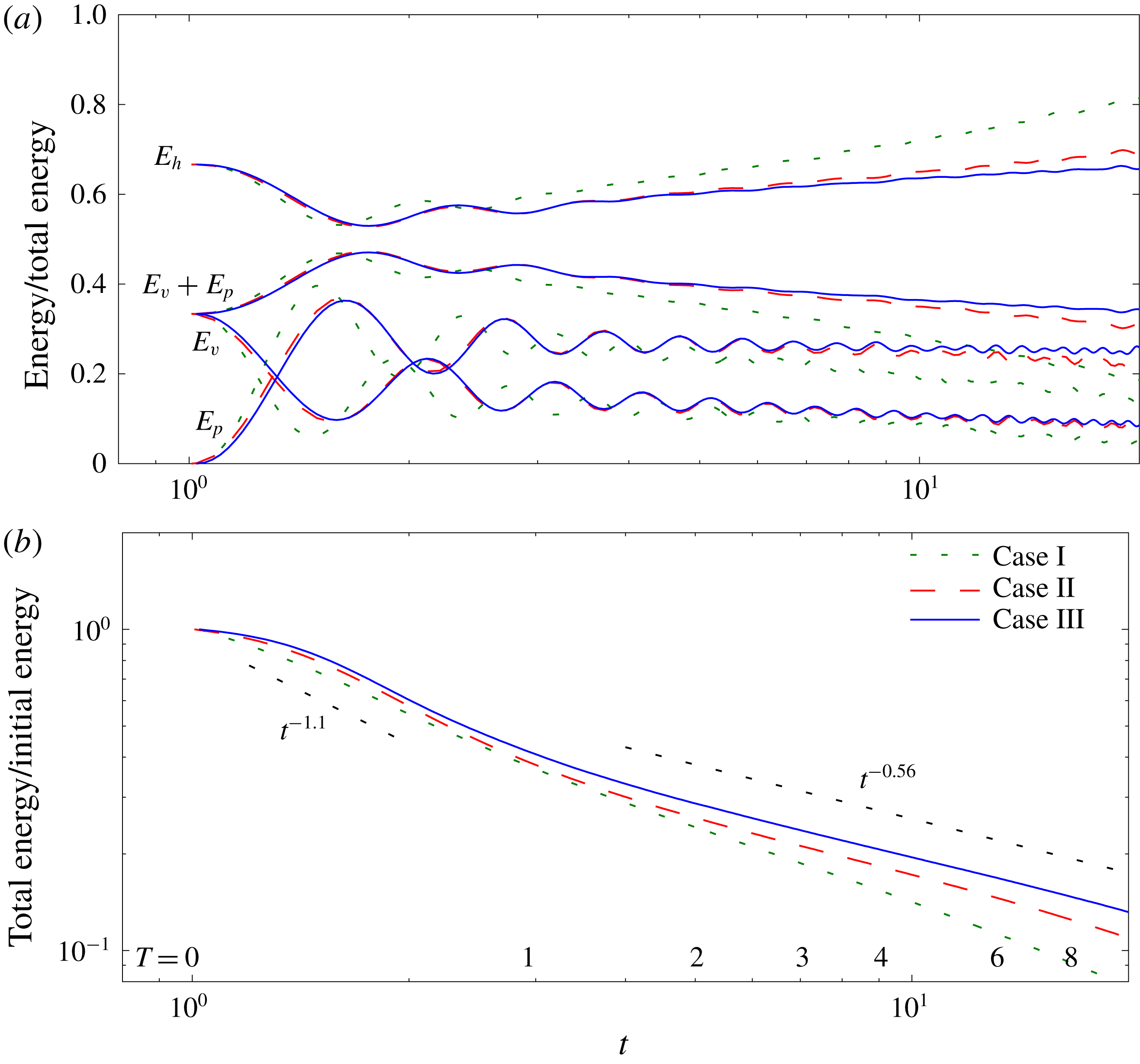
Information regarding the energy decay rates is given in figure 5. Here
 $E_{h}$
is the kinetic energy associated with
 $u$
and
 $v$
, and
 $E_{v}$
is that associated with
 $w$
. We define
 $E_{p}$
, the potential energy of the density fluctuations relative to the ambient density, as
 $$\begin{eqnarray}E_{p}=\frac{1}{2}\left(\frac{2\unicode[STIX]{x03C0}}{Fr}\right)^{2}\unicode[STIX]{x1D70C}^{\prime 2}.\end{eqnarray}$$
 $E_{p}$
can be considered as a surrogate for available potential energy (Lorenz Reference Lorenz1955). In panel (a) of the figure, all the energies have been normalised by the local (in time) total energy, i.e. by
 $E_{h}+E_{v}+E_{p}$
. From this panel it is observed that the horizontal components of the kinetic energy become increasingly dominant over the sum of the vertical component and the potential energy. This could be due to one or more of several effects. Possibly internal waves are being absorbed by the more horizontal motions, as in the laboratory experiments of Godoy-Diana et al. (Reference Godoy-Diana, Chomaz and Billant2004), leading to a decrease in both
 $E_{v}$
and
 $E_{p}$
while enhancing
 $E_{h}$
. Furthermore, as kinetic energy is exchanged with potential energy through the action of the buoyancy flux
 $-(2\unicode[STIX]{x03C0}/Fr)^{2}\langle \unicode[STIX]{x1D70C}w\rangle$
, with
 $\langle \cdot \rangle$
denoting a spatial average over the entire domain, the dissipation rate of potential energy
 $\unicode[STIX]{x1D712}$
(see § 3.1.4) provides another avenue for dissipation in addition to the kinetic energy dissipation rate
 $\unicode[STIX]{x1D716}$
. From this panel, it is also observed that the partition between the contributions to total energy depends on the Reynolds number, since Reynolds number is the only parameter that is varied between the simulations. This Reynolds number dependence is not surprising. For example, Perot & de Bruyn Kops (Reference Perot and de Bruyn Kops2006) reported, from examining many sources, that the decay exponents for non-stratified turbulence are larger in magnitude for lower Reynolds numbers. Finally, note from panel (b), and the fact that the non-stratified energy decay rate is approximately
 $t^{-1.1}$
, that the decay rate of the total energy is inhibited by the stratification, consistent with the inhibition of the decay rates of the horizontal components of the velocity.
(a) Ratio of energy contributions to total energy versus time. (b) Total energy versus time. In places where it is difficult to see the curves for Case II, they almost coincide with those for Case III. In (b), the two reference slopes correspond to
 $n=-0.55$
and
 $n=-0.28$
in figure 2(c).

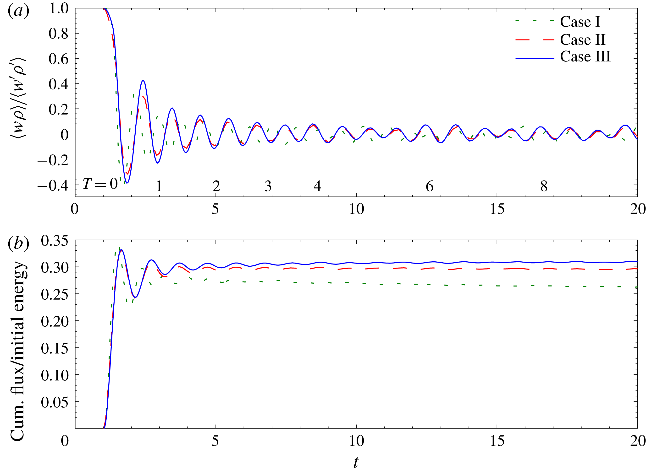
The behaviour of the buoyancy flux for all three stratified cases is seen in figure 6. The oscillations about 0 in the buoyancy flux in figure 6(a) represent net exchanges from the vertical component of the kinetic energy to potential energy (positive values) and back from potential into kinetic energy (negative values), consistent with the plots of these components of the energy, and corresponding to the noted oscillations in
 $w^{\prime }$
and
 $\unicode[STIX]{x1D70C}^{\prime }$
. These oscillatory results are qualitatively consistent with the numerical simulations of Riley et al. (Reference Riley, Metcalfe, Weissman and West1981) and the laboratory experiments of Liu (Reference Liu1995). Figure 6(b) is a plot of the cumulative (integrated) value of the buoyancy flux, divided by the initial total energy, giving the net transfer of kinetic into potential energy. It is seen that, for cases II and III, the cumulative flux asymptotes to approximately 30 % of the initial total energy. Also note that the cumulative flux is somewhat smaller for Case I, the lowest Reynolds number case. These facts are closely related to the behaviour of the mixing efficiency
 $\unicode[STIX]{x1D702}$
discussed in the next section.
(a) Buoyancy flux, normalised by
 $w^{\prime }\unicode[STIX]{x1D70C}^{\prime }$
, versus time for all three stratified cases. (b) Cumulative buoyancy flux normalised by initial total energy.

3.1.4 Dissipation rates and mixing efficiency
The dissipation rates of potential and kinetic energies are
 $$\begin{eqnarray}\unicode[STIX]{x1D712}=\frac{1}{PrRe}\left(\frac{2\unicode[STIX]{x03C0}}{Fr}\right)^{2}\langle \unicode[STIX]{x1D735}\unicode[STIX]{x1D70C}\boldsymbol{\cdot }\unicode[STIX]{x1D735}\unicode[STIX]{x1D70C}\rangle\end{eqnarray}$$
and
 $$\begin{eqnarray}\unicode[STIX]{x1D716}=\frac{1}{Re}\langle \unicode[STIX]{x1D64E}:\unicode[STIX]{x1D64E}\rangle ,\end{eqnarray}$$
respectively, where
 $\unicode[STIX]{x1D64E}$
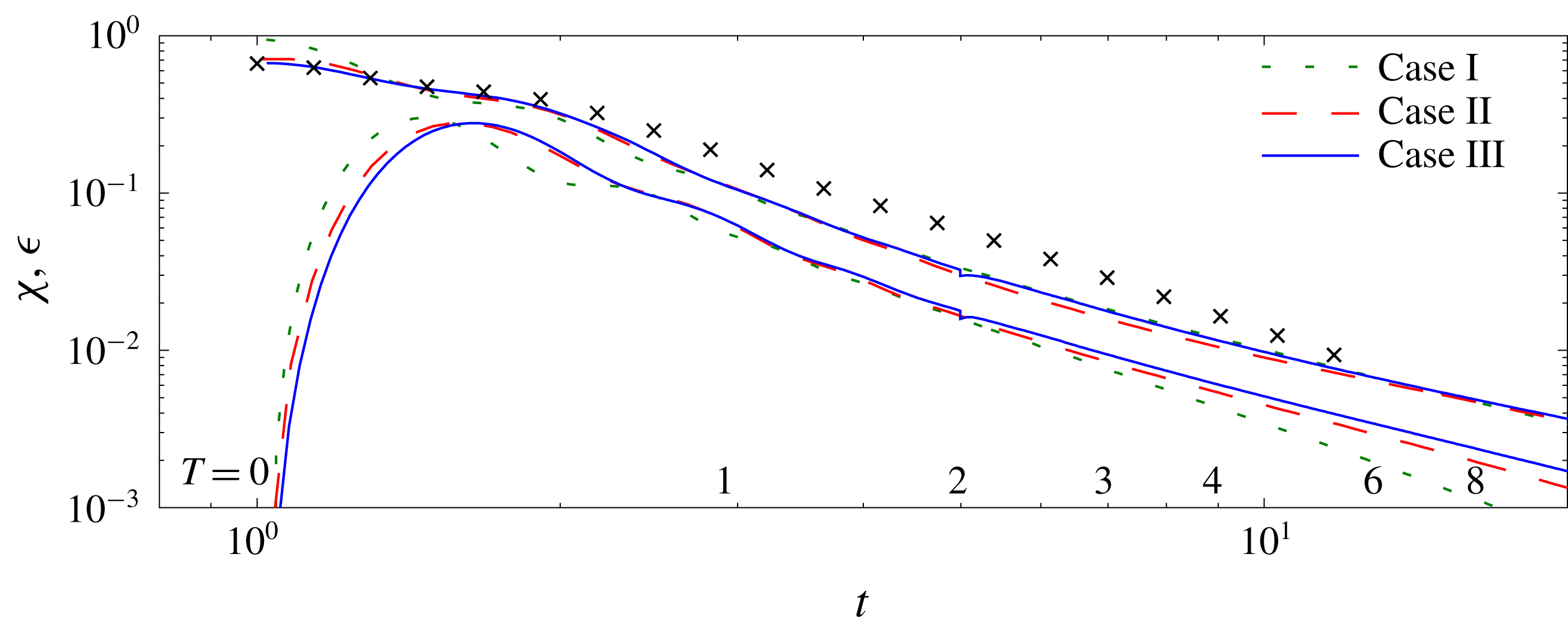
is the non-dimensional strain rate tensor. The time evolutions of their volume averages are shown in figure 7. Noticeable is the decrease in
 $\unicode[STIX]{x1D716}$
due to the stratification. Furthermore, there is a slight decrease and then increase in
 $\unicode[STIX]{x1D716}$
as the Reynolds number is increased, whereas there is a slight increase in
 $\unicode[STIX]{x1D712}$
as it is increased. Also evident is that the non-stratified cases are not quite in power-law decay at
 $t=1$
, which is also apparent in figure 2 for all the non-stratified cases; however, power-law decay does occur in the non-stratified simulations well before
 $T=1$
. In addition note that, after the flow adjustment, the ratio of
 $\unicode[STIX]{x1D712}$
to
 $\unicode[STIX]{x1D716}$
is approximately 0.54 except for the lowest Reynolds number case (Case I), where the ratio continues to decrease in time. We will find below in § 3.2 that, for this lowest Reynolds number case, the flow might not be fully turbulent beyond approximately 2 buoyancy periods.
Values of
 $\unicode[STIX]{x1D716}$
(upper curves),
 $\unicode[STIX]{x1D712}$
(lower curves). Symbols are for Case III with no stratification.

Of special interest is the ratio
 $\unicode[STIX]{x1D702}\equiv \unicode[STIX]{x1D712}/(\unicode[STIX]{x1D712}+\unicode[STIX]{x1D716})$
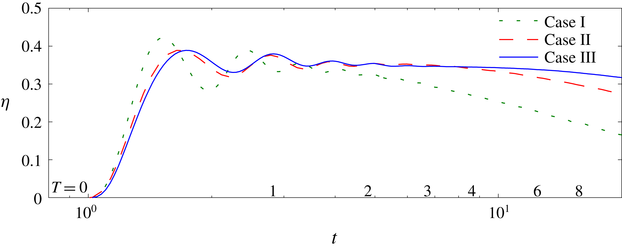
, which is sometimes taken to be the definition of the mixing efficiency (Osborn Reference Osborn1980; Smyth, Moum & Caldwell Reference Smyth, Moum and Caldwell2001). From figure 8 it is seen that, for the higher Reynolds number cases,
 $\unicode[STIX]{x1D702}$
asymptotes to a value of approximately 0.35, compared to the value of 0.3 obtained by Riley & de Bruyn Kops (Reference Riley and de Bruyn Kops2003) in a similar regime, to 0.25 obtained by Maffioli, Brethouwer & Lindborg (Reference Maffioli, Brethouwer and Lindborg2016) at very low Froude number, to 0.41 inferred from the data of Liu (Reference Liu1995), and 0.17 assumed by Osborn (Reference Osborn1980) based upon ocean data. In the forced homogeneous simulations reported by Almalkie & de Bruyn Kops (Reference Almalkie and de Bruyn Kops2012b
),
 $\unicode[STIX]{x1D702}$
is approximately 0.36 for
 $Fr_{h}=$
between 0.258 to 1.47. Note that the value for
 $\unicode[STIX]{x1D702}$
of 0.35 is consistent with the asymptotic ratio of
 $\unicode[STIX]{x1D712}/\unicode[STIX]{x1D716}$
of approximately 0.54 indicated by figure 7.
Mixing efficiency
 $\unicode[STIX]{x1D702}=\unicode[STIX]{x1D712}/(\unicode[STIX]{x1D712}+\unicode[STIX]{x1D716})$
.

There is some evidence that
 $\unicode[STIX]{x1D702}$
depends on the Prandtl (or Schmidt) number. For example, from numerical simulations of stratified shear flows, Smyth et al. (Reference Smyth, Moum and Caldwell2001) found that
 $\unicode[STIX]{x1D702}$
decreased from 0.35 to 0.22 as the Prandtl number increased from 1 to 7. More recently Salehipour & Peltier (Reference Salehipour and Peltier2015) found in numerical simulations of stratified shear flows that
 $\unicode[STIX]{x1D702}$
decreased from 0.24 to 0.18 as the Prandtl number increased from 1 to 16. Salehipour & Peltier (Reference Salehipour and Peltier2015) also gave some physical and mathematical reasoning for this decrease with Prandtl number. For a subset of the simulations of de Bruyn Kops, Riley & Portwood (Reference de Bruyn Kops, Riley and Portwood2016) run with
 $Pr=7$
,
 $\unicode[STIX]{x1D702}$
ranges from 0.17 at
 $Fr_{h}=0.4$
to 0.28 at
 $Fr_{h}=2.8$
.
3.1.5 The buoyancy Reynolds number and activity parameter
Dimensional reasoning suggests that three initial parameters are required to describe decaying, homogeneous, stratified turbulence. For equations (2.2), these are chosen to be the Prandtl number,
 $Pr$
, in addition to the Reynolds and Froude numbers,
 $Re$
and
 $Fr$
. The latter are defined here in terms of the integral length scale
 $\hat{L}$
and r.m.s. velocity
 $\hat{U}$
of the simulated flow at
 $t=1$
, i.e. before there is any effect of stratification. The conditions at
 $t=1$
provide a useful basis for non-dimensionalising the flow statistics. To better understand the effects of stable stratification, however, it is useful to consider the local in time values of
 $Re$
and
 $Fr$
. Because of the non-isotropy which develops in the flows, the corresponding vertical and horizontal scales in the flow differ significantly, as seen in figure 3. Therefore, considering the local r.m.s. horizontal velocity
 $u_{h}$
, one can define two Froude numbers of potential importance,
 $Fr_{h}=2\unicode[STIX]{x03C0}u_{h}/NL_{ux}$
and
 $Fr_{v}=2\unicode[STIX]{x03C0}u_{h}/NL_{uz}$
based upon the horizontal longitudinal integral scale
 $L_{ux}$
and the vertical lateral integral scale
 $L_{uz}$
, respectively.
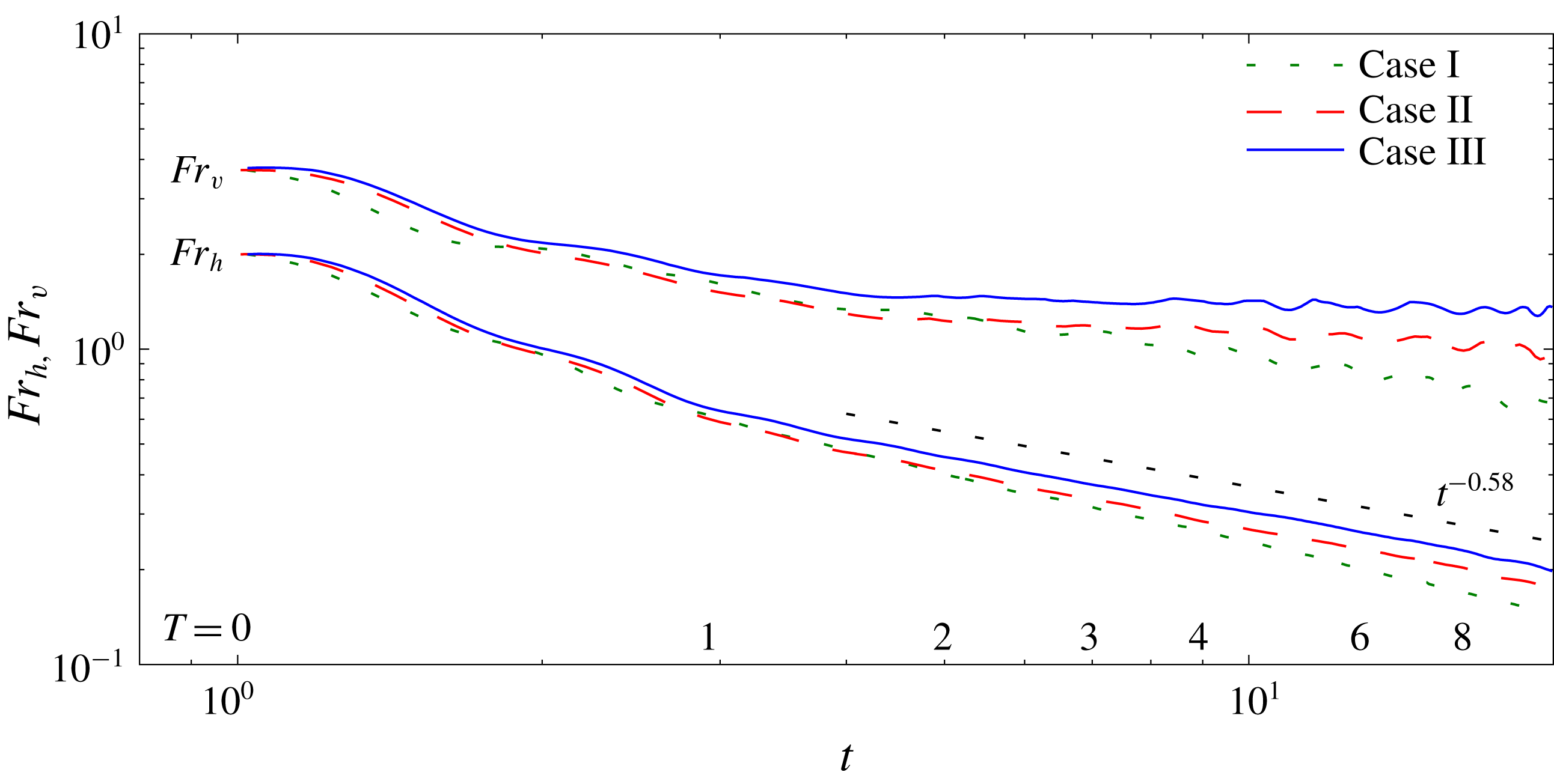
Horizontal and vertical Froude numbers,
 $Fr_{h}$
and
 $Fr_{v}$
respectively, versus time
 $t$
.

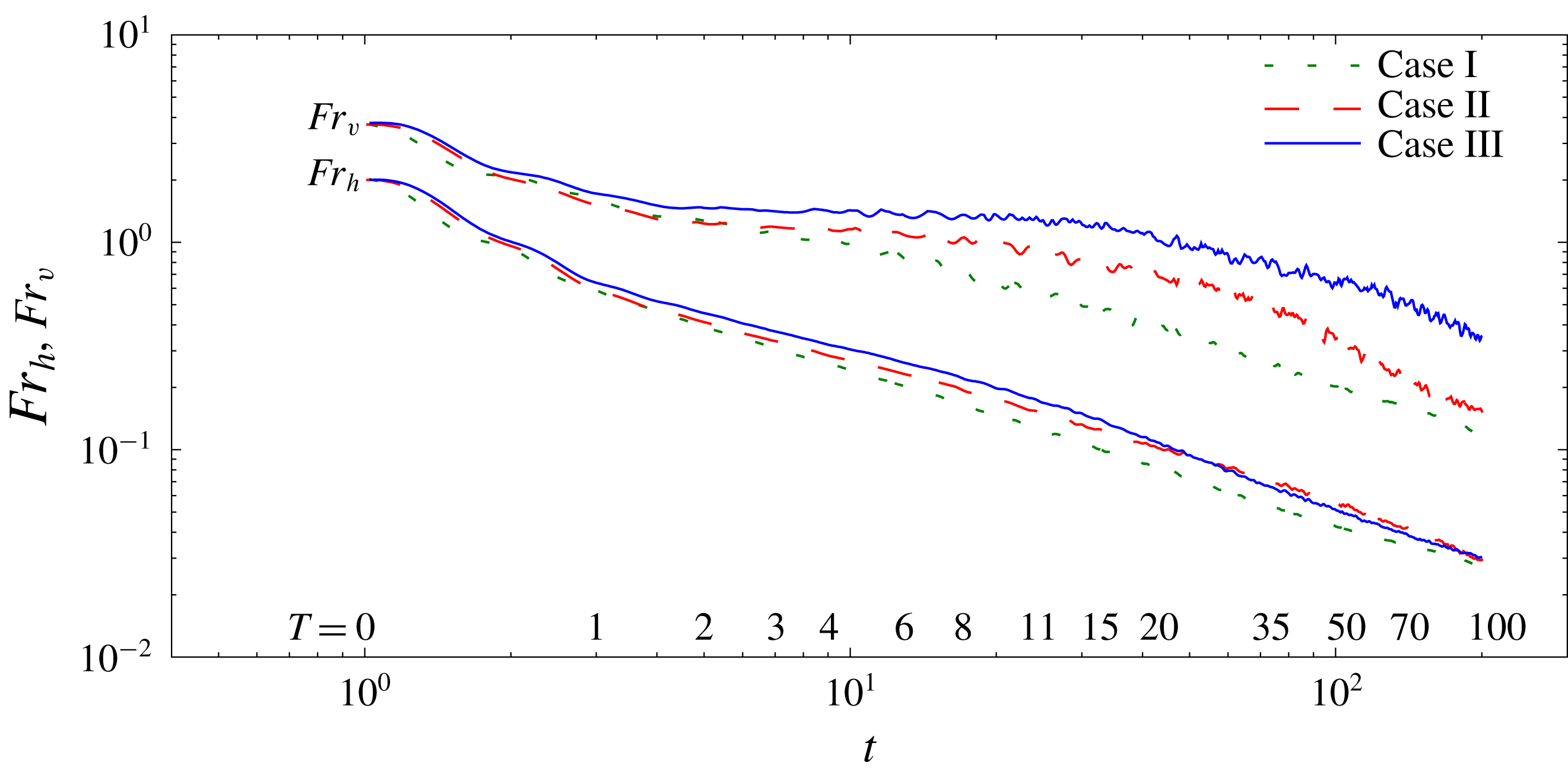
The temporal decay of the horizontal Froude number,
 $Fr_{h}$
, and the vertical Froude number,
 $Fr_{v}$
, are seen in figure 9 for all three cases. The decay curves for both Froude numbers are very similar for all three different Reynolds numbers, although at later times the Froude numbers for Case I are decaying slightly faster. Furthermore, as suggested by Riley et al. (Reference Riley, Metcalfe, Weissman and West1981),
 $Fr_{h}<O(1)$
for about
 $T>1$
, indicating that stratification begins to dominate in this temporal region. This is consistent with the results in figures 2 and 3, where the velocity decay rates and integral scale growth rates change somewhat abruptly near
 $T=1$
, as the flows enter the strongly stratified regime. On the other hand, the scaling arguments of Billant & Chomaz (Reference Billant and Chomaz2001) suggest that when
 $Fr_{h}<O(1)$
, at least for large
 $Re$
, then
 $Fr_{v}$
should become and remain
 $O(1)$
. This is also seen to occur in figure 9. More discussion of the late time behaviour of both
 $Fr_{h}$
and
 $Fr_{v}$
is presented in § 3.2.
Since
 $Fr_{v}$
becomes approximately constant for
 $T>1$
, its local in time behaviour need not be considered. Therefore, it is important to locally consider only
 $Re_{h}$
and
 $Fr_{h}$
, where
 $Re_{h}$
is also based upon
 $u_{h}$
and
 $L_{ux}$
. As reviewed in § 1, these two parameters combine to form
 ${\mathcal{R}}=Fr_{h}^{2}Re_{h}$
, whose potential relevance is based on the shearing dynamics observed to occur when strong stratification leads to the tendency for vertical decoupling of horizontal motions (Riley & de Bruyn Kops Reference Riley and de Bruyn Kops2003).
In the stratified turbulence literature,
 ${\mathcal{R}}$
is often referred to as the ‘buoyancy Reynolds number’, a terminology we have adopted in this paper. In the geophysical literature, this terminology usually denotes
 $$\begin{eqnarray}Gn\equiv \frac{\hat{\unicode[STIX]{x1D716}}}{\hat{\unicode[STIX]{x1D708}}\hat{N^{2}}}=Fr_{t}^{2}Re_{t}.\end{eqnarray}$$
Here the turbulence Froude and Reynolds numbers,
 $Fr_{t}$
and
 $Re_{t}$
, are defined in terms of the turbulence length scale
 $\hat{\ell }=\hat{U} ^{3}/\hat{\unicode[STIX]{x1D716}}$
, with
 $\hat{U}$
being the total r.m.s. velocity. These are the definitions used in Brethouwer et al. (Reference Brethouwer, Billant, Lindborg and Chomaz2007); however, they refer to
 $Gn$
as the buoyancy Reynolds number. (Note then that
 ${\mathcal{R}}$
and
 $Gn$
differ in the choice of their characteristic velocity and characteristic length scales.) We use the symbol
 $Gn$
in deference to the introduction of this quantity by Gibson (Reference Gibson and Nihous1980), and to its identification by Gargett, Osborn & Nasmyth (Reference Gargett, Osborn and Nasmyth1984) as a measure of the scale separation available for turbulence between the Ozmidov,
 $\hat{L}_{o}=(\hat{\unicode[STIX]{x1D716}}/\hat{N}^{3})^{1/2}$
, and Kolmogorov,
 $\hat{L}_{k}=(\unicode[STIX]{x1D708}^{3}/\hat{\unicode[STIX]{x1D716}})^{1/4}$
, length scales; we call
 $Gn$
the ‘activity parameter’ following some of the early literature on the subject (e.g. Dillon & Caldwell Reference Dillon and Caldwell1980).
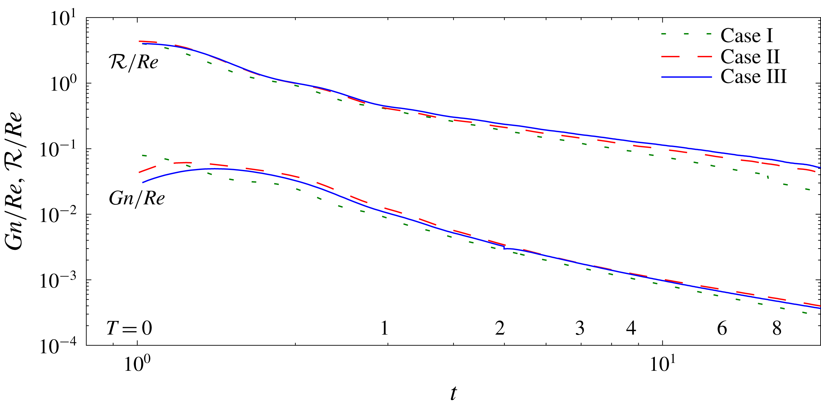
Values of
 ${\mathcal{R}}$
and
 $Gn$
, normalised by the initial Reynolds number, versus
 $t$
.

In figure 10 the evolution of
 ${\mathcal{R}}$
and
 $Gn$
in time are shown. Note that, as seen in terms of their decay rates in figure 10,
 ${\mathcal{R}}$
and
 $Gn$
are not proportional in the present simulations, so that they cannot be used interchangeably. Also note that there is a change in slope in
 ${\mathcal{R}}$
at about
 $T=1$
, consistent with the results for
 $u$
and
 $v$
seen in figure 2. It is also apparent that
 ${\mathcal{R}}$
scaled by the initial Reynolds number evolves differently for Case I than for Cases II and III. All three cases evolve in a similar manner up to about
 $T=2$
, at which point Cases II and III appear to diverge from Case I.
Our hypothesis is that the differences in the evolution of the three cases, evident in figure 10, can be explained by when
 $Gn$
drops below
 $O(1)$
, as will be discussed more in § 3.2 on late time results. Gibson (Reference Gibson and Nihous1980) predicted that
 $Gn>30$
is necessary for sustained turbulence, a value supported experimentally by Stillinger et al. (Reference Stillinger, Helland and Van Atta1983). In simulations of forced homogeneous stratified turbulence with
 $Gn=13,48$
and 220 (Portwood et al.
Reference Portwood, de Bruyn Kops, Taylor, Salehipour and Caulfield2016), only in the case with
 $Gn=220$
is there a range of length scales in which the turbulence is approximately isotropic throughout much of the simulation domain, although all the cases exhibit at least some patches of approximately isotropic turbulence. For the same data, de Bruyn Kops (Reference de Bruyn Kops2015) shows that, even in the case with
 $Gn=220$
, there is no range of scales consistent with the assumptions of Kolmogorov, Oboukhov and Corrsin regarding inertial and convective subranges (Kolmogorov Reference Kolmogorov1941; Oboukhov Reference Oboukhov1941a
,Reference Oboukhov
b
, Reference Oboukhov1949; Corrsin Reference Corrsin1951; Kolmogorov Reference Kolmogorov1962; Oboukhov Reference Oboukhov1962). For the same three data sets, Portwood et al. (Reference Portwood, de Bruyn Kops, Taylor, Salehipour and Caulfield2016) find that at
 $Gn=220$
the domain is dominated by space-filling patches of turbulence, while when
 $Gn=13$
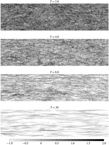
and 48 the simulated flows consist of a mixture of space-filling patches and horizontally layered turbulence. As seen in figures 1 and 11, the flows studied here become very layered beyond approximately
 $T=2$
.
Value of
 $\log _{10}(Gn)$
on a vertical slice of Case III at various times. Only the upper
 $1/4$
and left
 $1/2$
of the domain is plotted.

3.2 Late time results
Turning now to
 ${\mathcal{R}}$
, Riley & de Bruyn Kops (Reference Riley and de Bruyn Kops2003) have argued that shear instabilities can be expected to occur in the strongly stratified regime provided
 ${\mathcal{R}}>O(1)$
. This criterion has been verified, to some extent, by the simulations of Deloncle, Billant & Chomaz (Reference Deloncle, Billant and Chomaz2008) and refined by Augier & Billant (Reference Augier and Billant2011). It is seen that, for all the cases and all the times,
 ${\mathcal{R}}/Re$
is greater than approximately 0.1, and so that, approximately,
 ${\mathcal{R}}>15$
, indicating that that we would expect shear instabilities to continue to exist for these flows. These instabilities would only be expected to lead to turbulence, however, when approximately
 $Gn>0.5$
.
Hebert & de Bruyn Kops (Reference Hebert and de Bruyn Kops2006a
) present data from 14 simulations of decaying stratified turbulence that indicate
 ${\mathcal{R}}\propto Gn$
, but each simulation is sampled at a single time, not as a function of time. For the current simulations, the plots of
 ${\mathcal{R}}$
and
 $Gn$
versus time in figure 10 indicate that
 $Gn$
decays more rapidly than does
 ${\mathcal{R}}$
for all three cases; therefore there is no proportionality between
 $Gn$
and
 ${\mathcal{R}}$
and, in all three cases, the ratio
 ${\mathcal{R}}/Gn$
increases with time. The ratio of
 $Gn$
to
 ${\mathcal{R}}$
is closely related to the ratio of the integral scale,
 $L_{h}$
, to the turbulence length scale,
 $\ell =U^{3}/\unicode[STIX]{x1D716}$
, i.e. the ratio
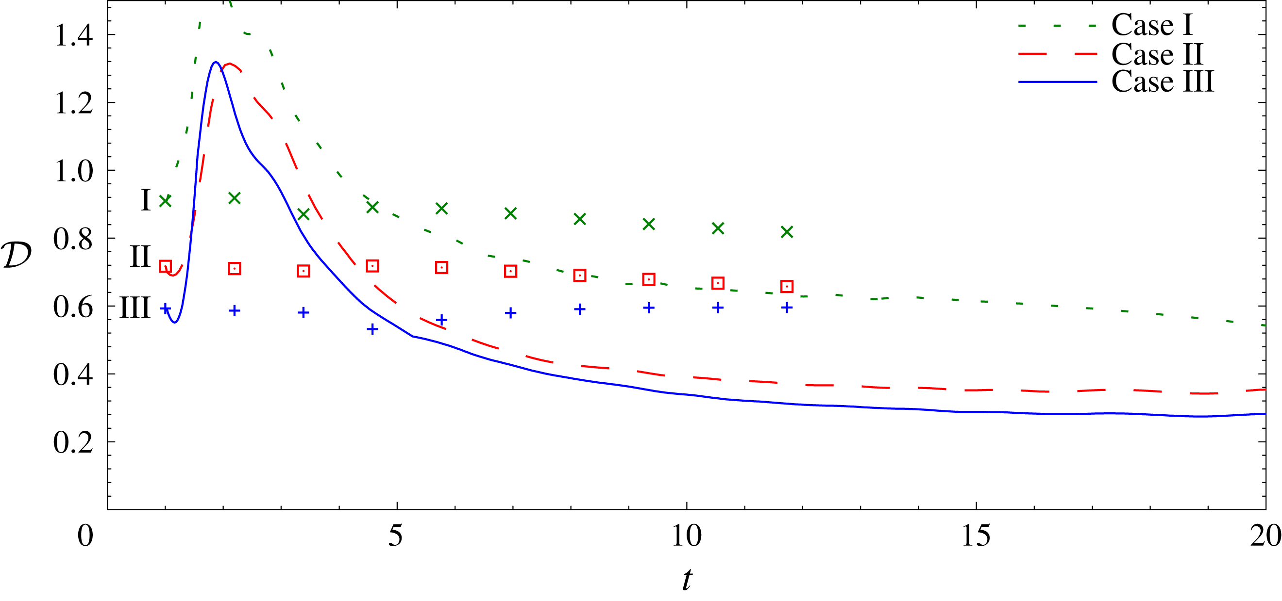
 $$\begin{eqnarray}{\mathcal{D}}\equiv \unicode[STIX]{x1D716}L_{h}/U^{3}.\end{eqnarray}$$
To be precise,
 $Gn/{\mathcal{R}}$
includes a factor of the ratio of the r.m.s. horizontal velocity to the r.m.s. total velocity, and there is an additional factor of
 $2\unicode[STIX]{x03C0}^{2}$
. The ratio
 ${\mathcal{D}}$
, however, is well known in the study of non-stratified turbulence and so we turn our attention to it rather than to
 $Gn/{\mathcal{R}}$
. Pope (Reference Pope2000) shows that, when the ratio is computed from a model spectrum, it depends on the Reynolds number over the range of Reynolds numbers accessed by all but a few numerical simulations and laboratory experiments in homogeneous, isotropic turbulence. From an examination of results from a number of laboratory experiments and numerical simulations, Sreenivasan (Reference Sreenivasan1998) reports
 ${\mathcal{D}}$
in the range of approximately 0.4 to 1.81. He also notes that simulations of homogeneous, isotropic turbulence by multiple researchers can be divided into two groups, with
 ${\mathcal{D}}$
for one group of simulations being consistent with each other but markedly higher than for the other group, for which
 ${\mathcal{D}}$
is consistent with the analysis of Pope. For decaying homogeneous stratified simulations, Maffioli & Davidson (Reference Maffioli and Davidson2016) report
 ${\mathcal{D}}$
as low as 0.3. Hebert & de Bruyn Kops (Reference Hebert and de Bruyn Kops2006a
) report
 ${\mathcal{D}}\approx 0.4$
for their snapshots of the 14 decaying cases referenced above. For the simulations of forced stratified turbulence with
 $Gn=13$
, 48 and 220, de Bruyn Kops (Reference de Bruyn Kops2015) reports
 ${\mathcal{D}}=0.53$
at
 $Gn=220$
and 0.57 at
 $Gn=13$
. Sreenivasan reports that
 ${\mathcal{D}}$
tends to be higher for forced cases. We note that typically in forced simulations, and certainly in those of de Bruyn Kops (Reference de Bruyn Kops2015), the large scales are not as well resolved as in decaying simulations, which adds to the difficulty in accurately estimating
 $L_{h}$
.
Data for
 ${\mathcal{D}}$
for the current simulations are shown in figure 12. For the non-stratified cases, the values are consistent with those collected by Sreenivasan (Reference Sreenivasan1998), and they exhibit the expected trend of increasing with decreasing Reynolds number from one simulation to the next. The results for the stratified cases go through an adjustment period at early time and then trend toward the range 0.3–0.4, consistent with the decaying cases of Hebert & de Bruyn Kops (Reference Hebert and de Bruyn Kops2006a
) and Maffioli & Davidson (Reference Maffioli and Davidson2016). The lower values of
 ${\mathcal{D}}$
for the stratified cases are consistent with the decrease in
 $\unicode[STIX]{x1D716}$
and the increase in both
 $u_{h}$
and
 $L_{h}$
.
Length scale ratio. The symbols are for the unstratified cases and the lines are for the stratified cases.

3.2.1 Energy spectra
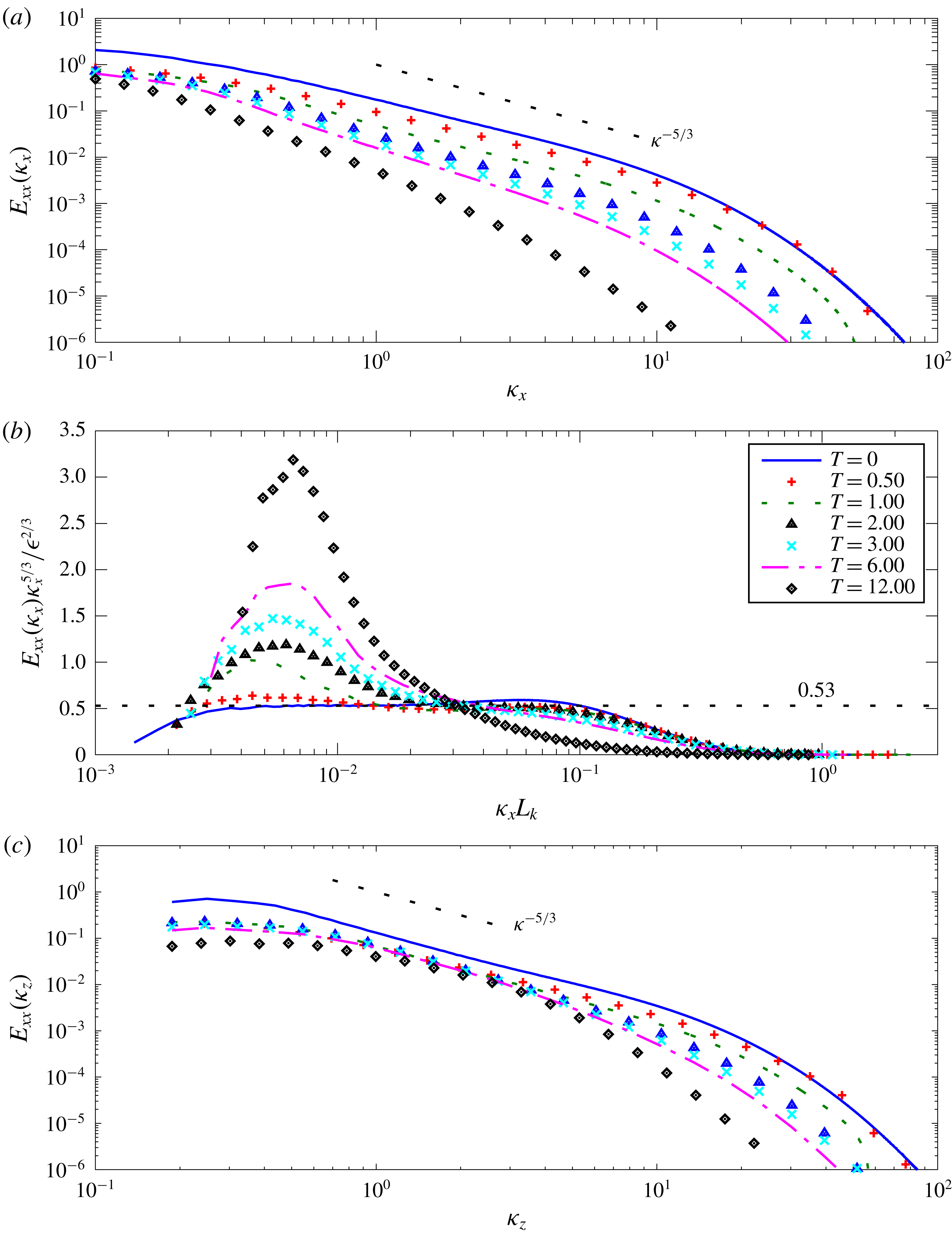
The horizontal velocity spectra
 $E_{xx}$
versus horizontal wavenumber
 $\unicode[STIX]{x1D705}_{x}$
are plotted in figure 13(a), where the spectra of
 $u$
have been averaged with the corresponding spectra of
 $v$
. The corresponding compensated horizontal spectra versus horizontal wavenumber times the Kolmogorov length scale
 $L_{k}$
are plotted in figure 13(b). The horizontal velocity spectra
 $E_{xx}$
versus vertical wavenumber
 $\unicode[STIX]{x1D705}_{z}$
are plotted in figure 13(c), again where the spectra of
 $u$
have been averaged with the corresponding spectra of
 $v$
. It is seen that, at
 $T=0$
, when the stratification is applied, the non-stratified spectra have moderate inertial subranges. The compensated spectrum in figure 13(b) is consistent with the Kolmogorov constant of approximately
 $C_{1}=0.53$
, which is slightly higher than the value of
 $0.49$
in Pope (Reference Pope2000) but well within the range for the many data sets reviewed by Sreenivasan (Reference Sreenivasan1995).
Uncompensated (a) and compensated (b) longitudinal spectra and uncompensated vertical spectrum (c) of
 $u$
averaged with that of
 $v$
for Case III.

In isotropic turbulence at high enough Reynolds numbers, there is found a bump in the compensated spectrum to the right of
 $\unicode[STIX]{x1D705}L_{k}\approx 0.02$
, which is sometimes attributed to a ‘bottleneck’ of energy transferring to smaller scales. Meyers & Meneveau (Reference Meyers and Meneveau2008) review efforts to understand and model this phenomenon. de Bruyn Kops (Reference de Bruyn Kops2015) shows that stratification suppresses this bump and that the
 $-5/3$
slope can occur at the top of the dissipation range even though it does not occur in the inertial range. The suppression of the bump by stratification is consistent with the hypothesis that the bump is due to the bottlenecking of the energy transfer rate combined with the observation that, for the current simulations, stratification reduces the energy decay rate, and hence the energy transfer rate.
Note that in figure 13(b) there is a bottleneck bump to the right of
 $\unicode[STIX]{x1D705}L_{k}\approx 0.02$
at
 $T=0$
. By
 $T=0.5$
the bump has been suppressed and a peak in the compensated spectrum has begun to develop in the range where the inertial-range plateau exists at
 $T=0$
. By
 $T=12$
, the compensated spectrum is very similar to those in figure 4(a) of de Bruyn Kops (Reference de Bruyn Kops2015). This is somewhat surprising because it has been assumed that the peak in the compensated spectra is an artefact of the energy forcing used to maintain the statistical stationarity of those simulations, yet in the current simulations there is no forcing. The plots of the compensated horizontal spectra are also qualitatively similar to those obtained by Maffioli & Davidson (Reference Maffioli and Davidson2016), and in addition the growth of the compensated spectra in the low wavenumber region, and the decay in the high wavenumber region, are also consistent.
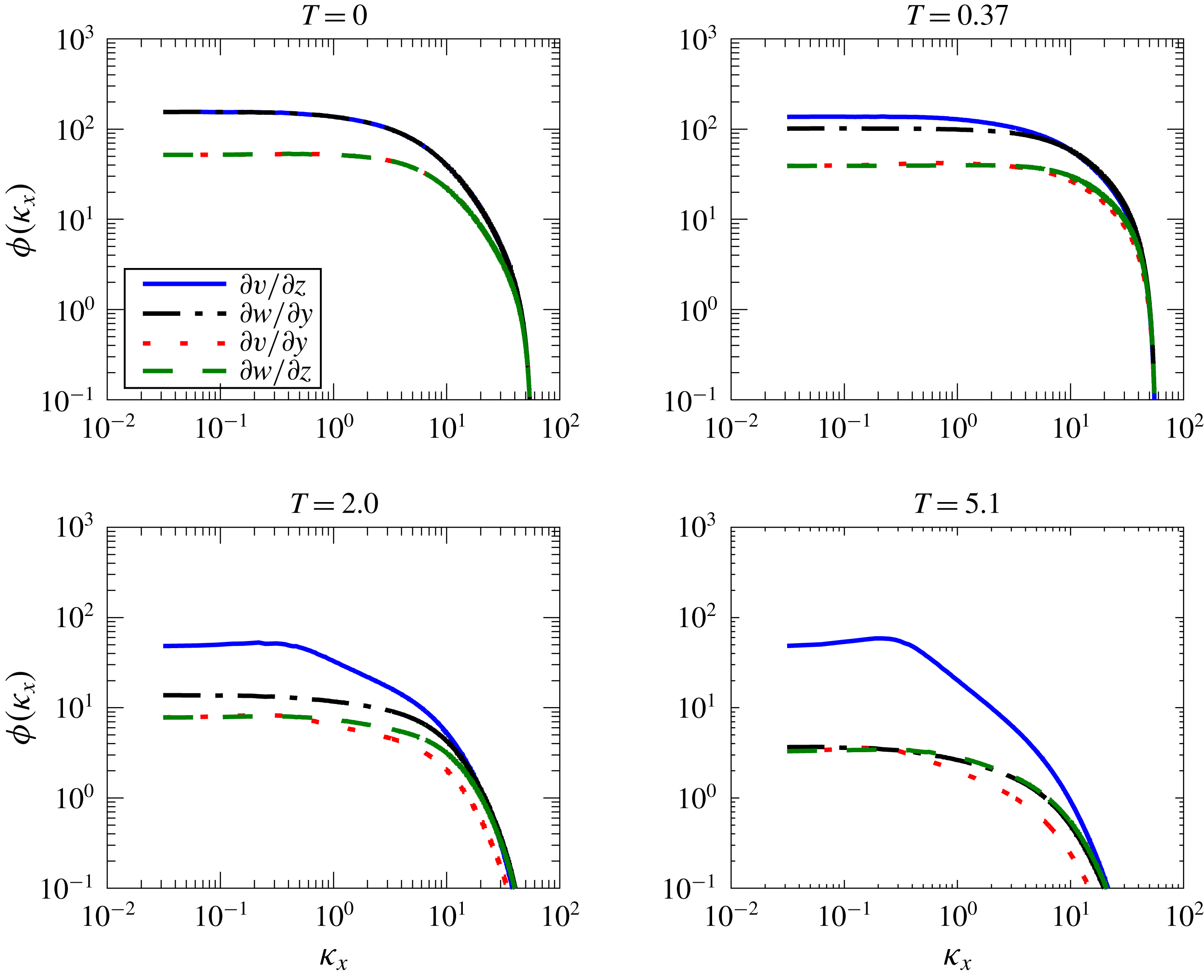
Horizontal spectra of various shear terms.

The question arises regarding whether a stratified turbulence inertial range, as proposed by Lindborg (Reference Lindborg2006), should be expected for our simulations. The possibility for this to occur will depend upon (i) the ratio of the energy-containing range scale, characterised by
 $L_{h}$
, to the Ozmidov scale
 $L_{o}$
; and (ii) the ratio of the Ozmidov scale to the Kolmogorov scale, given by
 $Gn^{4/3}$
. A stratified turbulence inertial range would be expected to exist between the energy-containing and Ozmidov wavenumbers, so that
 $L_{h}/L_{o}$
should be at least 100 or more. Furthermore, for turbulent behaviour to exist, we find in § 3.2 that
 $Gn$
must be at least of order 1. Considering the highest Reynolds number case (Case III), we find that at
 $T=1$
, where the flow becomes strongly affected by stratification,
 $L_{h}/L_{o}=32.3$
, while
 $L_{o}/L_{k}=10.1$
. Clearly the ratio of
 $L_{h}/L_{o}$
is not large enough for an inertial range to exist. When the ratio of
 $L_{h}/L_{o}$
becomes large enough for the inertial range to exist, at
 $T=6$
, where
 $L_{h}/L_{o}=216$
, then
 $L_{o}/L_{k}$
has dropped to 1.4, which is too small to expect active turbulence. Therefore we conclude that there is not enough separation of scales for a stratified flow inertial range to occur. The flow would have to be started at a substantially higher Reynolds number for the possibility to exist.
A comparison of the horizontal and vertical wavenumber spectra in figures 13(a) and 13(c) give some insight into the turbulence dynamics. The high wavenumber energy in the horizontal decays much more rapidly in time than does the vertical wavenumber energy. On the other hand, the low wavenumber energy in the horizontal decays much more slowly. These facts together indicate a much weaker spectral energy transfer in the horizontal than in the vertical, a fact qualitatively consistent with the arguments of Lilly (Reference Lilly1983) and Billant & Chomaz (Reference Billant and Chomaz2001). Note that at higher wavenumbers the vertical spectra steepen considerably at later times, consistent with the flow layering. A clear
 $k_{z}^{-3}$
spectrum is not obtained, however.
Some additional insight into the dynamics of strongly stratified flows can be seen from examining the horizontal spectra of various components of the velocity gradient tensor. Figure 14 contains plots of the
 $k_{x}$
spectra of
 $\unicode[STIX]{x2202}v/\unicode[STIX]{x2202}z$
,
 $\unicode[STIX]{x2202}w/\unicode[STIX]{x2202}y$
,
 $\unicode[STIX]{x2202}v/\unicode[STIX]{x2202}y$
and
 $\unicode[STIX]{x2202}w/\unicode[STIX]{x2202}z$
for four points in time for Case III, the highest Reynolds number case. Note that, for isotropic turbulence, it is expected that the spectra of
 $\unicode[STIX]{x2202}v/\unicode[STIX]{x2202}z$
and
 $\unicode[STIX]{x2202}w/\unicode[STIX]{x2202}y$
will be identical, as will the spectra of
 $\unicode[STIX]{x2202}v/\unicode[STIX]{x2202}y$
, and
 $\unicode[STIX]{x2202}w/\unicode[STIX]{x2202}z$
. It is clear that at
 $T=0$
this is the case. As the flow evolves, the spectra of
 $\unicode[STIX]{x2202}v/\unicode[STIX]{x2202}y$
, and
 $\unicode[STIX]{x2202}w/\unicode[STIX]{x2202}z$
remain approximately the same, although the spectrum of
 $\unicode[STIX]{x2202}v/\unicode[STIX]{x2202}y$
decreases slightly faster than that of
 $\unicode[STIX]{x2202}w/\unicode[STIX]{x2202}z$
at higher wavenumbers. This supports the scaling arguments of Billant & Chomaz (Reference Billant and Chomaz2001) that all three terms in the continuity equation,
 $\unicode[STIX]{x2202}u/\unicode[STIX]{x2202}x$
,
 $\unicode[STIX]{x2202}v/\unicode[STIX]{x2202}y$
and
 $\unicode[STIX]{x2202}w/\unicode[STIX]{x2202}z$
, should be of the same order. Somewhat surprisingly, the spectra of
 $\unicode[STIX]{x2202}w/\unicode[STIX]{x2202}y$
and
 $\unicode[STIX]{x2202}w/\unicode[STIX]{x2202}z$
become almost identical at the latest time. What is noteworthy, however, is the rapid decrease with time of the spectra for
 $\unicode[STIX]{x2202}w/\unicode[STIX]{x2202}y$
,
 $\unicode[STIX]{x2202}v/\unicode[STIX]{x2202}y$
and
 $\unicode[STIX]{x2202}w/\unicode[STIX]{x2202}z$
compared to that for
 $\unicode[STIX]{x2202}v/\unicode[STIX]{x2202}z$
, with the spectrum for
 $\unicode[STIX]{x2202}v/\unicode[STIX]{x2202}z$
evolving well above the rest. Furthermore, the peak in the spectrum of
 $\unicode[STIX]{x2202}v/\unicode[STIX]{x2202}z$
remains into smaller wavenumbers. Both of these facts are indications of the development of strong vertical shearing of the horizontal motions as suggested by Lilly (Reference Lilly1983).
We now consider the late time behaviour of these flows, when
 $Gn$
falls to
 $O(1)$
and below, and so viscosity becomes a dominating influence. Figure 11 contains grey scale plots, for the same conditions as in figure 1, of the turbulence activity parameter
 $Gn$
, defined in (3.5), which gives an indication of the strength of the turbulence. Although at
 $T=0.5$
the effects of stable stratification are little noticeable, by two and especially four buoyancy periods a quasi-horizontal nature and a patchiness of the turbulence are clearly evident. By
 $T=30$
, at which point
 $Gn$
is well below 1 (see figure 16 below) the behaviour of the flow has substantially changed.
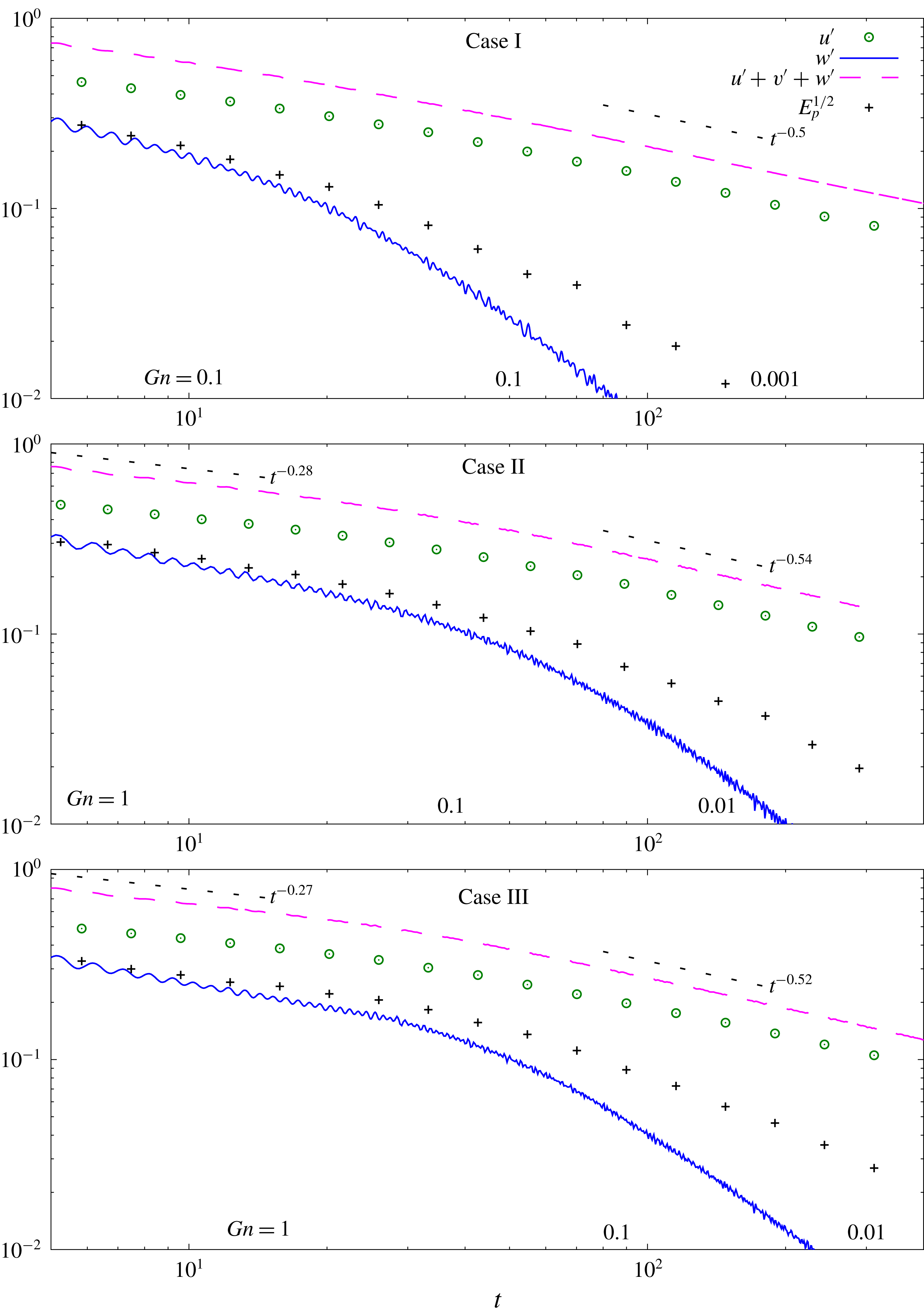
Figure 15 contains plots of
 $u^{\prime }$
,
 $w^{\prime }$
and
 $E_{p}^{1/2}$
versus time carried out to 150 buoyancy periods or more for each case, and where
 $Gn$
has dropped to values of 0.01 or less at very late times. The
 $Gn$
scale at the bottom of each plot gives the local values of
 $Gn$
at different times for each case. There are two things to note about these plots. First, for each case, for values of
 $Gn$
between 1 and 0.1,
 $u^{\prime }$
begins to decay at a slightly steeper rate. Second, for values of
 $Gn$
in this same range, the vertical velocity and
 $E_{p}^{1/2}$
(proportional to
 $\unicode[STIX]{x1D70C}^{\prime }$
) begin to decay precipitously, indicating that the flows are becoming quasi-horizontal.
Evolution of
 $u^{\prime }$
,
 $v^{\prime }$
, and
 $E_{p}^{1/2}$
into late time. Reference slopes are shown for
 $Gn>1$
and
 $Gn\ll 1$
except for Case I
 $Gn>1$
which is not in the range of times on this figure. For velocity data at early times see figure 2.

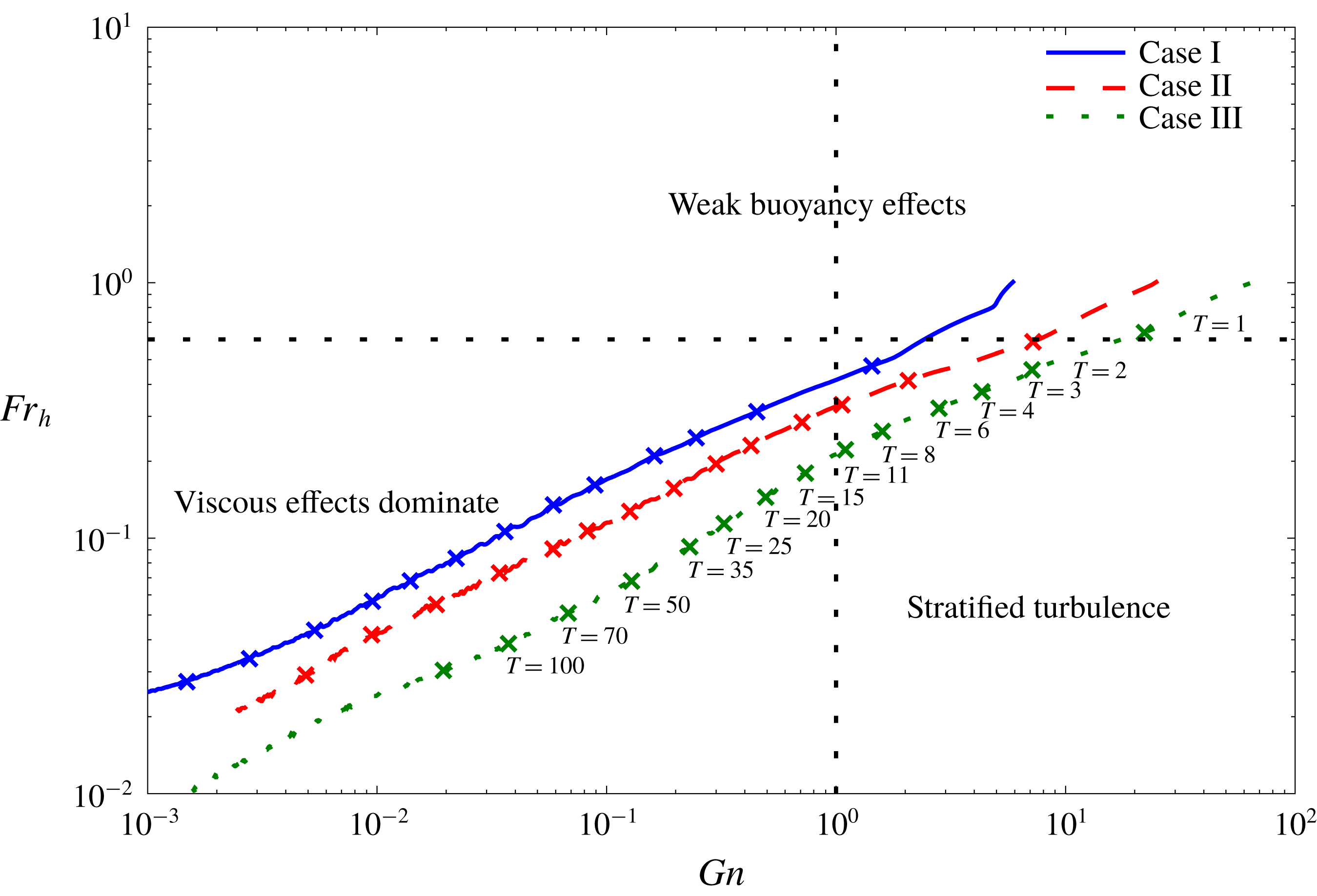
These plots can be better understood by examining the trajectory of each flow in the
 $Fr_{h}$
–
 $Gn$
plane, as given in figure 16. Each flow is seen to go through three regimes. In the first, the flows decay at the non-stratified rate, which is seen in figure 2 to occur up to approximately 1 buoyancy period after flow initiation, when the values of the local Froude numbers have fallen to approximately 0.6 (see figure 9). We take this to be the value of
 $Fr_{h}$
when a flow has entered the strongly stratified regime. The decay rate in this regime diminishes due to the effects of stable stratification, approximately as predicted by Davidson (Reference Davidson2010). Finally, in the third regime, when
 $Gn$
has decayed to between 1 and 0.1 for each case, the flows become viscously dominated and begin to decay at a faster rate. Note that this viscous domination had already been observed for Case I at earlier times in the behaviour of
 $\unicode[STIX]{x1D70C}^{\prime }$
in figure 4, in the behaviour of the various components of energy in figure 5(a), and in the behaviour of the mixing efficiency in figure 8.
The trajectory of each flow in the
 $Fr_{h}$
–
 $Gn$
plane. The symbols mark the time in buoyancy periods, with the corresponding times indicated on the curve for Case III.

These results are analogous to those obtained in the experiments of Spedding (Reference Spedding1997) discussed in § 1. He studied the decay of turbulence in the wake of a towed sphere in a salt-stratified towing tank, and found in measuring the mean axial velocity that, initially, the flow decayed at the non-stratified rate. But at a time of the order of a buoyancy period, the decay rate decreased appreciably in what he called the non-equilibrium regime. Further in time, in the region he called the late wake, or quasi-two-dimensional regime, the flow again decayed at a faster rate. We speculate that in this last regime
 $Gn$
had become small in his flows, which would therefore be viscously dominated. Furthermore the vertical velocity had been suppressed compared to the horizontal velocity, as the flows exhibited quasi-horizontal vortex structure.
Froude numbers versus time.

Additional insight can be gained by examining the behaviours of the Froude numbers, based upon the horizontal and vertical integral scales, throughout the flow decay, as shown in figure 17. The Froude number based upon the horizontal integral scale,
 $Fr_{h}$
, is seen to continually decay, although the decay is somewhat diminished when the effects of stratification become strong, and then the decay becomes stronger as viscous effects begin to dominate. At first the Froude number based upon the vertical scale,
 $Fr_{v}$
, begins to decay at a rate similar to that of
 $Fr_{h}$
. As the effects of stratification become strong, however,
 $Fr_{v}$
becomes approximately constant, as predicted by the scaling arguments of Billant & Chomaz (Reference Billant and Chomaz2001), and as seen in the simulations of Maffioli & Davidson (Reference Maffioli and Davidson2016). Later in time, as the effects of viscosity begin to dominate, then
 $Fr_{v}$
begins to decay.
Based upon our simulation results, we find that it is most useful and instructive to divide up the flows into three different regimes, depending upon the values of
 $Fr_{h}$
and
 $Gn$
. When
 $Fr_{h}>O(1)$
the flows behave almost as non-stratified flows and we term this regime the weakly stratified regime. When
 $Fr_{h}$
becomes less than
 $O(1)$
, in our case less than approximately 0.6 which occurs at approximately one buoyancy period, stratification begins to strongly affect the flows, and we term this the strongly stratified regime, as discussed in § 1. Depending on the local value of
 $Gn$
, the strongly stratified regime splits into two parts. When
 $Gn$
is greater than
 $O(1)$
, the flow obeys the decay laws predicted by Davidson (Reference Davidson2010), and the scaling arguments predicted by Billant & Chomaz (Reference Billant and Chomaz2001), and we call this the stratified turbulence regime, in deference to the terminology introduced by Lilly (Reference Lilly1983). Finally, in the strongly stratified regime, when
 $Gn$
has dropped somewhat below 1, the flows become quasi-horizontal, and the dissipation rate is approximately governed by the vertical shearing of the horizontal velocity, and we refer to this as the viscous-dominated regime.
The behaviour of the flow in this late time, viscous-dominated regime can be seen from the scaling arguments of Riley et al. (Reference Riley, Metcalfe, Weissman and West1981), as modified by Godoy-Diana et al. (Reference Godoy-Diana, Chomaz and Billant2004) to include the effects of viscosity. The arguments suggest that the ratio of the r.m.s. vertical velocity to the r.m.s. horizontal velocity should be proportional to
 $Fr_{h}/Fr_{v}$
, so that the flow should be quasi-horizontal in this regime. Godoy-Diana et al. (Reference Godoy-Diana, Chomaz and Billant2004) also argued that as
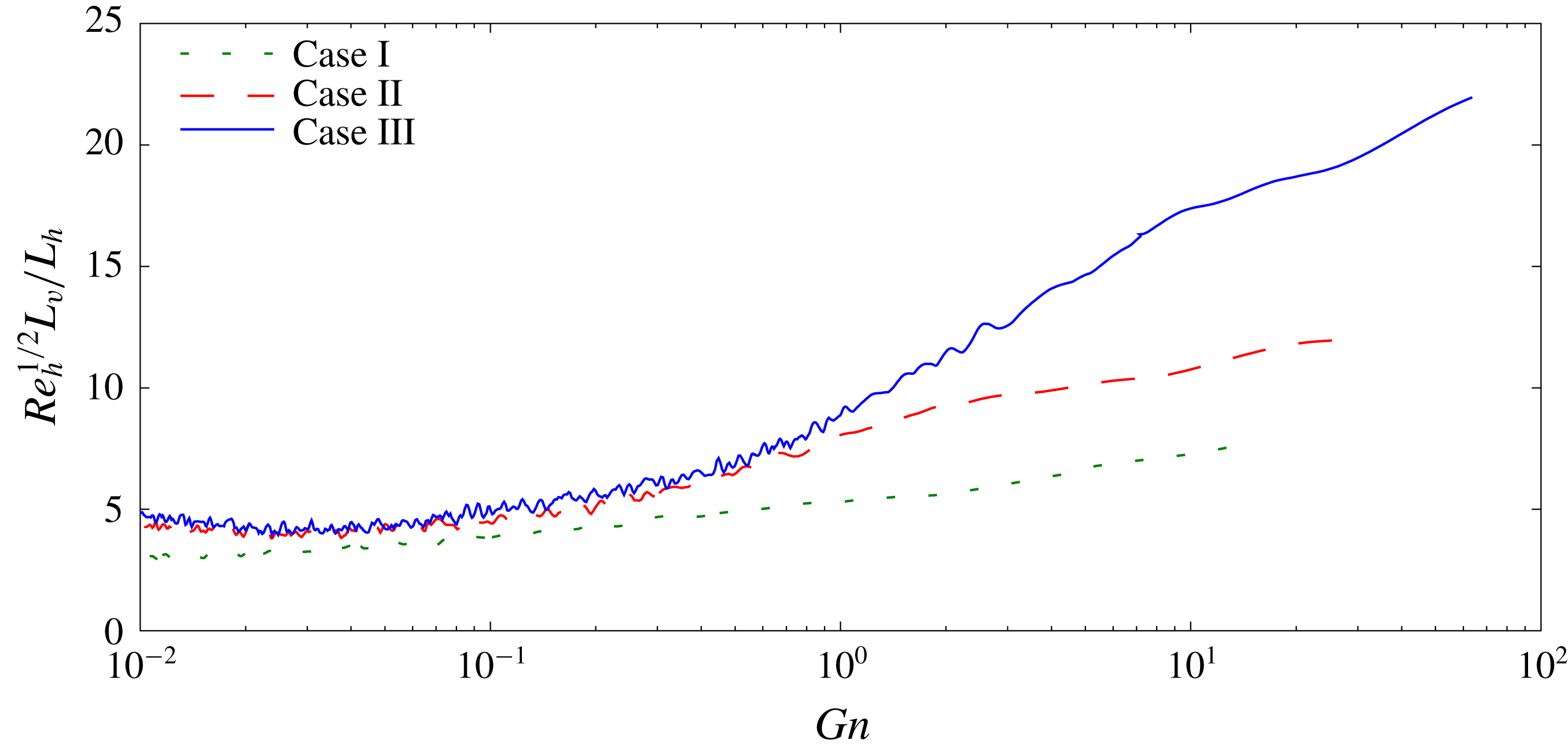
 $Gn$
becomes small, the vertical viscous term in the horizontal momentum equation becomes large compared to the vertical transport term, suggesting that the vertical integral scale behaves as
 $L_{v}=L_{h}Re_{h}^{-1/2}$
, where
 $Re_{h}$
is defined in terms of
 $L_{h}$
. Figure 18 is a plot of the ratio
 $Re_{h}^{1/2}L_{v}/L_{h}$
versus
 $Gn$
for Cases I, II and III. It is seen that for approximately
 $Gn>O(1)$
, this ratio is not constant, but increases as
 $Gn$
increases. As
 $Gn$
decreases below
 $O(1)$
, however, the ratio becomes approximately constant with a value slightly below 5, and in fact the curves for Cases I and II collapse together, although the value for Case I is somewhat lower. This gives some confidence in the arguments of Godoy-Diana et al. (Reference Godoy-Diana, Chomaz and Billant2004) applies to these simulated flows.
A test of the relationship
 $L_{v}=L_{h}Re_{h}^{-1/2}$
for small
 $Gn$
.

Examining these arguments further, neglecting the vertical transport term and assuming that the aspect ratio
 $L_{v}/L_{h}$
is small as suggested by the scaling arguments and by figure 17, so that the horizontal diffusion terms can be neglected, the result is that (2.2) reduce to
 $$\begin{eqnarray}\displaystyle & \displaystyle \frac{\unicode[STIX]{x2202}}{\unicode[STIX]{x2202}t}\boldsymbol{u}+\boldsymbol{u}_{h}\boldsymbol{\cdot }\unicode[STIX]{x1D735}_{h}\boldsymbol{u}_{h}=-\unicode[STIX]{x1D735}_{h}p+\frac{1}{Re}\frac{\unicode[STIX]{x2202}^{2}\boldsymbol{u}_{h}}{\unicode[STIX]{x2202}z^{2}}, & \displaystyle\end{eqnarray}$$
 $$\begin{eqnarray}\displaystyle & \displaystyle 0=-\left(\frac{2\unicode[STIX]{x03C0}}{Fr}\right)^{2}\unicode[STIX]{x1D70C}-\frac{\unicode[STIX]{x2202}p}{\unicode[STIX]{x2202}z}, & \displaystyle\end{eqnarray}$$
 $$\begin{eqnarray}\displaystyle & \displaystyle \unicode[STIX]{x1D735}_{h}\boldsymbol{\cdot }\boldsymbol{u}_{h}=0, & \displaystyle\end{eqnarray}$$
 $$\begin{eqnarray}\displaystyle & \displaystyle \frac{\unicode[STIX]{x2202}\unicode[STIX]{x1D70C}}{\unicode[STIX]{x2202}t}+\boldsymbol{u}_{h}\boldsymbol{\cdot }\unicode[STIX]{x1D735}_{h}\unicode[STIX]{x1D70C}=\frac{1}{RePr}\frac{\unicode[STIX]{x2202}^{2}\unicode[STIX]{x1D70C}}{\unicode[STIX]{x2202}z^{2}}. & \displaystyle\end{eqnarray}$$
 $Gn$
. One is the fact that the flows are approximately horizontal, i.e.
 $u^{\prime }$
,
 $v^{\prime }\gg w^{\prime }$
, which in the present case is clearly indicated in figure 15. Another indication can be found by examining the ratios
 $$\begin{eqnarray}\displaystyle & \displaystyle Rt_{G}=\frac{15\unicode[STIX]{x1D708}}{4\unicode[STIX]{x1D716}}\left\langle \left(\frac{\unicode[STIX]{x2202}u}{\unicode[STIX]{x2202}z}\right)^{2}+\left(\frac{\unicode[STIX]{x2202}v}{\unicode[STIX]{x2202}z}\right)^{2}\right\rangle , & \displaystyle\end{eqnarray}$$
 $$\begin{eqnarray}\displaystyle & \displaystyle Rt_{D}=\frac{15\unicode[STIX]{x1D708}}{2\unicode[STIX]{x1D716}}\left\langle \left(\frac{\unicode[STIX]{x2202}u}{\unicode[STIX]{x2202}x}\right)^{2}+\left(\frac{\unicode[STIX]{x2202}v}{\unicode[STIX]{x2202}y}\right)^{2}\right\rangle , & \displaystyle\end{eqnarray}$$
 $$\begin{eqnarray}\displaystyle & \displaystyle Rt_{H}=\frac{15\unicode[STIX]{x1D708}}{4\unicode[STIX]{x1D716}}\left\langle \left(\frac{\unicode[STIX]{x2202}u}{\unicode[STIX]{x2202}y}\right)^{2}+\left(\frac{\unicode[STIX]{x2202}v}{\unicode[STIX]{x2202}x}\right)^{2}\right\rangle , & \displaystyle\end{eqnarray}$$
 $$\begin{eqnarray}\displaystyle & \displaystyle Rt_{M}=\frac{15\unicode[STIX]{x1D708}}{4\unicode[STIX]{x1D716}}\left\langle \left(\frac{\unicode[STIX]{x2202}w}{\unicode[STIX]{x2202}x}\right)^{2}+\left(\frac{\unicode[STIX]{x2202}w}{\unicode[STIX]{x2202}y}\right)^{2}\right\rangle , & \displaystyle\end{eqnarray}$$
 $$\begin{eqnarray}\displaystyle & \displaystyle Rt_{V}=\frac{15\unicode[STIX]{x1D708}}{\unicode[STIX]{x1D716}}\left\langle \left(\frac{\unicode[STIX]{x2202}w}{\unicode[STIX]{x2202}z}\right)^{2}\right\rangle . & \displaystyle\end{eqnarray}$$
 $Rt_{G}$
must be approximately
 $15/4$
. In contrast, in isotropic turbulence, all of the preceding ratios should be unity. Both of these conditions are observed in figure 19, which shows the ratios for case II. At early times, each of the ratios is approximately unity whereas at late time
 $Rt_{G}$
appears to by asymptoting to
 $15/4$
.
Plot of the five statistically independent contributions to
 $\unicode[STIX]{x1D716}$
, normalised as in (3.8), for Case II.

The results from other studies exhibit this behaviour of the dissipation rate as well. Both Fincham et al. (Reference Fincham, Maxworthy and Spedding1996) and Praud et al. (Reference Praud, Fincham and Sommeria2005) performed experiments in salt-stratified tanks, and both generated turbulence by towing a vertical grid through the tank. At the later stages of decay in both experiments the value of
 $Gn$
had dropped to values well below one. In addition, the flows had become approximately horizontal, and in both experiments it was reported that the ratio
 $Rt_{G}/(15/4)$
was well above 0.9. These features for both experiments all indicate the approximate validity of (3.7) at later times. Hebert & de Bruyn Kops (Reference Hebert and de Bruyn Kops2006b
) performed direct numerical simulations in a strongly stratified fluid of the decay of flows initially consisting of Taylor–Green vortices, similar to the work of Riley & de Bruyn Kops (Reference Riley and de Bruyn Kops2003), but over a very broad range of Reynolds number, Froude number and
 $Gn$
. They found that the ratio
 $Rt_{G}$
is a very strong function of
 $Gn$
, and that
 $Rt_{G}/(15/4)$
being near 0.9 only occurred when
 $Gn$
was order one or less. From the present results, and from these experimental and numerical results, there is reason to speculate that (3.7) hold in many other flows that are strongly stratified and
 $Gn$
is small.
4 Conclusions and discussion
Direct numerical simulations were used to study the effects of stable ambient density stratification on initially isotropic turbulence. To initialise the stratified flows, and for comparison with cases with stratification, first of all three non-stratified cases were run at three different Reynolds numbers. It was found that all three flows attained approximately self-similar decay, with r.m.s. decay rates of approximately
 $t^{-0.56}$
, and integral scale growth rates of approximately
 $t^{0.44}$
. These values are not far from the rates of
 $t^{-0.6}$
and
 $t^{0.4}$
predicted for Saffman turbulence (Saffman Reference Saffman1967), and observed in some laboratory data. Therefore, these non-stratified cases are useful for the initialisation of and comparison with the cases with stratification.
In the cases with stable stratification, analogous to the results of Spedding (Reference Spedding1997), as the flows decay we find that they traverse three different regimes which depend on the local Froude number,
 $Fr_{h}$
, and activity parameter,
 $Gn$
. In the first regime, the weakly stratified regime, which occurs up to approximately one buoyancy period, when
 $Fr_{h}$
is above about 0.6, the flows follow their non-stratified counterparts. By about one buoyancy period, however, the flows have adjusted to the stable stratification as the value of
 $F_{h}$
falls below 0.6. If
 $Gn$
remains high enough, then the flows enter the second regime, which we term the stratified turbulence regime, and proceed to decay in a manner similar to that predicted by Davidson (Reference Davidson2010), and to satisfy the scaling analysis of Billant & Chomaz (Reference Billant and Chomaz2001). In particular, the horizontal r.m.s. velocity decay rates are reduced, the growth rates of the horizontal integral scales of the horizontal velocities increase, while the vertical integral scales of the horizontal velocities begin to decrease. Finally, when the activity parameter decays to a value in the range of 0.1 to 1, the flows enter into the third regime, the viscous-dominated regime. Here the flow dynamics has changed considerably and follows the scaling analysis of Godoy-Diana et al. (Reference Godoy-Diana, Chomaz and Billant2004). In particular the vertical velocity becomes very small compared to the horizontal velocities, and the kinetic energy dissipation rate is dominated by the vertical shearing of the horizontal motions.
The results regarding the decrease in decay rate in the stratified turbulence regime are at least qualitatively consistent with the data from several laboratory experiments (Lin & Pao Reference Lin and Pao1979; Stillinger et al.
Reference Stillinger, Helland and Van Atta1983; Yoon & Warhaft Reference Yoon and Warhaft1990; Spedding Reference Spedding1997). They are inconsistent, however, with the results of several other laboratory experiments (Itsweire et al.
Reference Itsweire, Helland and Van Atta1986; Liu Reference Liu1995; Praud et al.
Reference Praud, Fincham and Sommeria2005). It is not clear why our results differ from some of the experimental results, and why in fact some of the experimental results differ from one another while performed under seemingly similar conditions. As mentioned in the introduction, a key difference between our simulations and the laboratory experiments is how the flows are initialised. Our flows have achieved close to a classical isotropic, homogeneous, decaying turbulent flow before the stratification is imposed. On the other hand in the laboratory experiments the stratification exists before the turbulence is generated. Generally in the laboratory experiments where a grid of mesh size
 $M$
is used to generate the turbulence, a certain distance from the grid, say
 $x_{0}/M$
, is required before the flow begins to decay in a self-similar manner. Taking
 $U$
to be the speed of the grid relative to the fluid, and with
 $t_{0}=x_{0}/U$
as the time it takes for the flow to become self-similar, then, in terms of buoyancy periods, this is
 $Nt_{0}/2\unicode[STIX]{x03C0}=(x_{0}/M)(NM/2\unicode[STIX]{x03C0}U)=(x_{0}/M)/Fr$
. In many of the laboratory experiments,
 $Fr\sim (x_{0}/M)$
, suggesting that the flows are often modified by stratification before they begin self-similar decay. These facts would suggest a change in decay behaviour different from what is obtained in our simulations; but it would not indicate how the decay rates would be different.
Another possible influence on the decay rates observed in the laboratory experiments is the Reynolds number. For example, the highest Taylor Reynolds numbers of the experiments quoted is 160 for the highest Reynolds number case of Praud et al. (Reference Praud, Fincham and Sommeria2005), which is about the same as for our intermediate case, Case II, of 158. Other examples are Yoon & Warhaft (Reference Yoon and Warhaft1990), who reported 36.7, and Liu (Reference Liu1995) with the value of 27.8. Based upon our results for Cases I and II, it would be expected that the viscous-dominated regime would be entered fairly early in the experiments, and therefore affects the decay rates. For example, in the kinetic energy decay plots of Praud et al. (Reference Praud, Fincham and Sommeria2005) (see their figure 4), the highest Taylor Reynolds number for the cases plotted is 81, corresponding to their cases bc and ad. Using the first data points in time plotted for each case, and an estimate of the dissipation rates taken from their figure 27, this gives estimates of
 $Gn$
in the range of 0.1 to 0.3. As seen from our figure 16, these values put the experiments in the viscously dominated regime.
There are several interesting features of the flows in the stratified turbulence regime. For example, the vertical component of the kinetic energy decays at a faster rate than the two horizontal components while, after its initial adjustment, the density fluctuation
 $\unicode[STIX]{x1D70C}^{\prime }$
decays at approximately the same rate as does
 $u_{h}$
. From an energetics perspective, this indicates that the potential energy decays at approximately the same rate as the horizontal components of the kinetic energy. This could be due to the density field trying to stay in cyclostrophic adjustment with the horizontal components of the velocity field. Another feature of this regime is the behaviour of the local Froude numbers; the Froude number
 $Fr_{h}$
continues to decay, while
 $Fr_{v}$
becomes approximately constant, consistent with the predictions of Billant & Chomaz (Reference Billant and Chomaz2001). Furthermore, in the stratified turbulence regime, for the two higher Reynolds number cases, the mixing efficiency asymptotes to approximately 0.35. This is roughly consistent with a number of numerical simulations with
 $Pr=O(1)$
(Smyth et al.
Reference Smyth, Moum and Caldwell2001; Riley & de Bruyn Kops Reference Riley and de Bruyn Kops2003; Almalkie & de Bruyn Kops Reference Almalkie and de Bruyn Kops2012b
; Maffioli et al.
Reference Maffioli, Brethouwer and Lindborg2016). The lowest Reynolds number case is only briefly in the stratified turbulence regime, however. After about 2 buoyancy periods its activity parameter has dropped well below 1 as it enters the viscous-dominated regime; its mixing efficiency as well as
 $F_{v}$
begin to decay.
The horizontal spectra of the horizontal components of the velocity behave very differently in the stratified cases compared to the non-stratified cases. Initially the spectra for these flows have a moderate inertial range, with a bump in the compensated spectra sometimes attributed to a ‘bottleneck’ in the energy transfer to smaller scales. As each flow evolves into the stratified turbulence regime, however, a peak in the compensated spectra arises and continues to grow at approximately wavenumber
 $\unicode[STIX]{x1D705}_{x}L_{k}=8\times 10^{-3}$
. In addition, in examining the horizontal spectra of various shear terms, it is found that the spectra of
 $\unicode[STIX]{x2202}u/\unicode[STIX]{x2202}x$
,
 $\unicode[STIX]{x2202}v/\unicode[STIX]{x2202}y$
and
 $\unicode[STIX]{x2202}w/\unicode[STIX]{x2202}z$
evolve in a very similar manner, again supporting the scaling arguments of Billant & Chomaz (Reference Billant and Chomaz2001). Even at moderate times the vertical shearing of the horizontal component of the velocity at somewhat low wavenumbers begins to dominate, indicating that vertical shear layers are probably driving the turbulence.
When
 $Fr_{h}$
is below 0.6 and the value of
 $Gn$
drops below between 1 and 0.1, the flows enter the third regime, the viscous-dominated regime. Here the flow dynamics changes again. Now the horizontal components of the velocity decay at a faster rate, similar to the decay rate in the first regime. In addition, the vertical velocity and density fluctuations decay at a much faster rate, as the flow becomes approximately horizontal. In this viscous-dominated regime, the flow behaviour appears to be consistent with (3.7), based upon the scaling arguments of Godoy-Diana et al. (Reference Godoy-Diana, Chomaz and Billant2004).
It should be mentioned that, as listed in table 1, a fourth case was simulated, Case IV, with the same initial Reynolds number as Case III, but with a different initial Froude number, in this case
 $Fr_{h}=1$
. This would possibly allow the examination of the effect of the initial Froude number, and would permit the flow to enter into the stratified turbulence regime earlier in time and so more energetic. Since the activity parameter is proportional to
 $1/\hat{N}^{2}$
, however, when the flow for Case IV enters into the stratified turbulence regime, its Froude number
 $Fr_{h}$
and activity parameter
 $Gn$
have almost identical values as for Case III, so that the flow behaviour was very similar to that of Case III. Therefore the results for Case IV are not presented.
Acknowledgements
We thank one of the referees for pointing out some important details regarding the energy decay rates in some of the laboratory experiments. This work was funded by the Office of Naval Research via grant N00014-15-1-2248. High performance computing resources were provided through the U.S. Department of Defense High Performance Computing Modernization Program by the Army Engineer Research and Development Center and the Army Research Laboratory under Frontier Project FP-CFD-FY14-007.