1. INTRODUCTION
A hospital always aims to provide the highest quality services at the lowest price. Operating rooms (ORs) are the greatest source of hospital revenue and strongly affect a hospital's overall performance (Guinet & Chaabane, Reference Guinet and Chaabane2003; Jebali et al., 2006; Al-Refaie, Judeh, & Chen, Reference Al-Refaie, Aldwairi and Chen2017). Scheduling and planning of surgeries is considered the most appropriate means of OR maintenance, which has recently received significant attention (Testi et al., Reference Testi, Tanfani and Torre2007; Devi et al., Reference Devi, Rao and Sangeetha2010; Al-Refaie, Chen, & Judeh, Reference Al-Refaie, Chen and Judeh2016). Souki (Reference Souki2011) studied operating theater scheduling with fuzzy periods. Two models were addressed; the first model objective was to minimize fuzzy operating theater completion time, whereas the second model objective was to minimize total fuzzy weighed patient completion time. Saadouli et al. (Reference Saadouli, Jerbi, Dammak, Masmoudi and Bouaziz2015) developed a daily scheduling technique consisting of two mathematical models for elective surgery optimization. Discrete event simulation was conducted in the orthopedic surgery division of a Tunisian hospital. Barbagallo et al. (Reference Barbagallo, Corradi, de Goyet, Iannucci, Porro, Rosso, Tanfani and Testi2015) formulated a three-phase approach to optimize operating theater activities for a hospital in Italy. However, most previous studies considered only single-objective models (Persson & Persson, Reference Persson and Persson2006; Nouaouri et al., Reference Nouaouri, Nicolas and Jolly2009), which do not reflect the complexity of scheduling concerns in real cases. In addition, the focus was primarily on immediate problems related to treating patients on the day of surgery (Jebali et al., 2006; Saadouli et al., Reference Saadouli, Jerbi, Dammak, Masmoudi and Bouaziz2015).
In practice, optimizing performance under fuzzy conditions becomes a real challenge to decision makers (Al-Refaie, Chen, & Al-Athamenh, Reference Al-Refaie, Chen and Al-Athamneh2016; Al-Refaie, Aldwairi, et al., Reference Al-Refaie, Judeh and Chen2017). Fuzzy goal programing has been found effective in dealing with uncertainty (Al-Refaie, Reference Al-Refaie2013, Reference Al-Refaie2015a , Reference Al-Refaie2015b ). It has been applied to optimize performance in several business applications (Al-Refaie, Reference Al-Refaie2014a , Reference Al-Refaie2014b , Reference Al-Refaie2014c ; Al-Refaie et al., Reference Al-Refaie, Diabat and Li2014). In this study, therefore, two optimization models will be developed for fuzzy scheduling and sequencing of ORs over multiple periods with the objective of minimizing overtime and undertime costs, and maximizing patient's preferences. The remaining of this study is outlined in the following sequence. Section 2 presents the development of the proposed optimization model. Section 3 provides applications of the developed models in a real-life case study. Section 4 discusses research results. Section 5 summarizes research conclusions and suggests future research.
2. PROPOSED OPTIMIZATION MODELS
2.1. OR scheduling
The OR department consists of S surgeons, P patients (p = 1, … , P), and R rooms (r = 1, … , R). The scheduling problem aims at determining by which surgeon s (s = 1, … , S), on which day t (t = 1, … , T), and in which room r (r = 1, … , R) the pth patient (p = 1, … , P) will be treated such that the patient's satisfaction about his/her scheduled date is maximized. The following assumptions are taken into consideration:
-
1. All ORs are identical; hence, a patient can be assigned to any OR provided that the required specialized equipment for his/her surgery is available.
-
2. Patient assignment to surgeons is predetermined according to their surgery needs.
-
3. Duration of surgery is deterministic, and it includes the whole time needed for a given surgery (including room preparation time, patient setup time, and cleaning time).
-
4. Patient's due date is less than the scheduled period.
-
5. Surgeon's availability and his/her regular working time and the maximum allowed overtime are all known and fixed.
The development of the fuzzy scheduling model considers the following two objectives with the associated constraints are built as follows.
2.1.1. Minimizing overtime and undertime
Let the decision variables OT rt and UT rt denote the overtime and undertime of room r on day t, respectively; r = 1, … , R, t = 1, … , T. The objective function is to minimize overtime (the amount of time for working after regular working hours in all ORs) and undertime (the amount of unused time). That is (1),
 $${\rm Min}\sum\limits_{t = 1}^T {\sum\limits_{r = 1}^R {{\rm O}{\rm T}_{rt}} } + \sum\limits_{t = 1}^T {\sum\limits_{r = 1}^R {{\rm U}{\rm T}_{rt}.} }$$
The main constraints are developed as follows:
-
1. The overtime, OT rt , in the rth room on tth day is equal to the summation of the duration, Tsur p , of all surgeries performed after the normal room working hours, α rt . Let λ rt denotes the availability matrix of room r on day t and let the binary decision variable, ξ prt , identify that the pth patient will be treated in the rth room on the tth day, such that it equals 1 if patient p is assigned to room r on day t and zero otherwise. Then (2),
(2) $${\rm O}{\rm T}_{rt} \ge \lambda _{rt}\left( {\sum\limits_{{\kern 1pt} p = 1}^P {\xi _{{\kern 1pt} prt} \times Tsur_p - \alpha _{rt}} } \right){\rm ,}{\mkern 1mu} \quad \forall r{\rm ,}\;t.$$
-
2. The undertime, UT rt , for rth room on day t should be less than the normal working hours, α rt . That is (3):
(3)
$${\rm U}{\rm T}_{rt} \ge \lambda _{rt}\left( {\alpha _{rt} - \sum\limits_{{\kern 1pt} p = 1}^P {\xi _{{\kern 1pt} prt} \times Tsur_p} } \right){\rm ,}{\mkern 1mu} \quad \forall r{\rm ,}\;t.$$
-
3. The overtime and undertime of room r on day t are always positive; or mathematically (4) and (5):
(4)
$${\rm O}{\rm T}_{rt} \ge 0{\rm ,}{\mkern 1mu} \quad \forall r{\rm ,}\;t{\rm ;}$$
(5)
$${\rm U}{\rm T}_{rt} \ge 0\comma \,\quad \forall r\comma \,t.$$
-
4. The total overtime incurred in room r on day t should not exceed the corresponding maximal overtime, O rt . That is (6),
(6)
$$\sum\limits_{\,p = 1}^P {({\rm \xi} _{\,prt} \times Tsur_p) -} \;{\rm \alpha} _{rt} \le O_{rt}\comma \,\quad \forall r\comma \,t.$$
-
5. The total duration of all surgeries carried out by surgeon s on day t should not exceed the maximum working time on that day, C st . Let the assigned surgeon s to patient p be expressed by a binary variable β ps . Mathematically (7),
(7)
$$\sum\limits_{\,p = 1}^P {\sum\limits_{r = 1}^R {{\rm \xi} _{\,prt} \times Tsur_p}} \times {\rm \beta} _{\,ps} \times {\rm \zeta} _{st} \le C_{st}\comma \,\quad \forall s\comma \,t.$$
-
6. Let ζ st matrix represent availability of surgeon s on day t, and η prt is the equipment availability for patient p in room r on day t. Patient p can be assigned to the available rooms, once the required equipment and surgeon are available as expressed in inequality (8).
(8)
$${\rm \xi} _{\,prt} \le {\rm \lambda} _{rt} \times {\rm \eta} _{\,prt} \times \sum\limits_{s = 1}^S {({\rm \beta} _{\,ps} \times {\rm \zeta} _{st})\comma \,\quad \forall r\comma \,p\comma \,t.} $$
-
7. Patient p is assigned before or at least on his or her due date (dint p ) and he or she should be assigned mostly once. Mathematically (9),
(9)
$$\sum\limits_{t = 1}^{{\rm Du}{\rm e}_p} {\sum\limits_{r = 1}^R {{\rm \xi} _{\,prt} \le 1}\comma \, \quad \forall p.} $$
-
8. The scheduled day should be after the hospitalization date. Those patients hospitalized on or before the first day of the scheduling period will not be scheduled on any day. However, patients hospitalized after the first day of the scheduling period cannot be assigned before their hospitalization date as follows (10):
(10)
$$\sum\limits_{t = 1}^{{\rm Ho}{\rm s}_p - 1} {\sum\limits_{r = 1}^R {{\rm \xi} _{\,prt} = 0}\comma \, \quad \forall p} \in [1\comma \,.\,.\,.\,\comma \,P]/{\rm Ho}{\rm s}_p \gt 1.$$
-
9. Let Day p denote the scheduled date of patient p, and M represent a very large number. The scheduled date of patient is t that complies with all the stated constraints that can be obtained from Eq. (11).
(11)
$$\eqalign{ {\rm Da}{\rm y}_p &= \sum\limits_{t = 1}^T {\sum\limits_{r = 1}^R {(t \times {\rm \xi} _{\,prt})}} {+ M} \cr & \quad \times \left( {1 - \sum\limits_{t = 1}^T {\sum\limits_{r = 1}^R {(t \times {\rm \xi}_{\,prt})}}} \right)\comma \quad \forall p.} $$
-
10. The variable of patients' assignment is a binary variable as expressed in Eq. (12):
(12)
$${\rm \xi} _{\,prt} \in \{ 0\comma \,1\}. $$


2.1.2. Maximizing patient's satisfaction
Case 1: The nominal-the-best (NTB) type satisfaction
Let P
N
denote patients assigned using this submodel and
 ${\rm Da}{\rm y}_{P_N}$
denote their scheduled date. The aim is to maximize patients' satisfaction for patients who have a specific preferable date such that their satisfaction will be 100% if they are assigned to that preferable date (
 ${\rm Da}{\rm y}_{o_{P_N}}$
). Then, the proper membership function is the NTB type. Let
 ${\rm \mu} \lpar {{\rm Da}{\rm y}_{P_N}} \rpar $
denotes the membership function that presents patient's satisfaction about his/her assigned date. Let
 $\Delta _{{\rm Da}{\rm y}_{P_N}}^ - $
and
 $\Delta _{{\rm Da}{\rm y}_{P_N}}^ + $
denote the maximal negative and positive permitted deviation from
 ${\rm Da}{\rm y}_{o_{P_N}}$
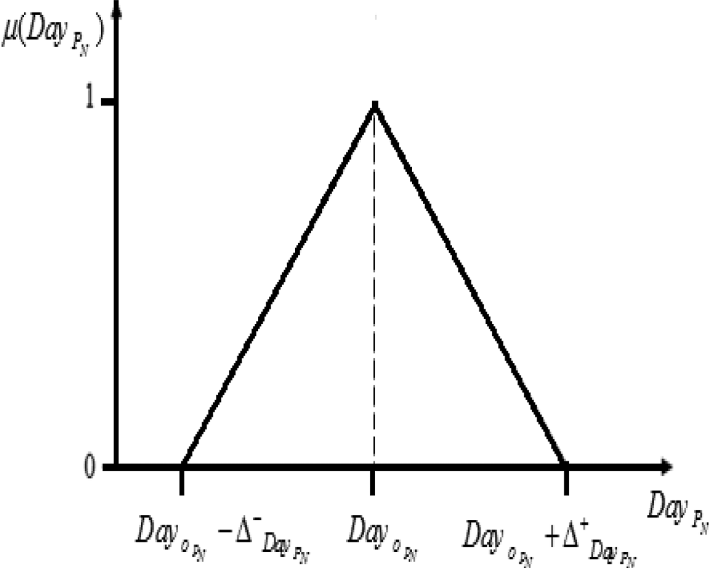
, respectively. The NTB function is demonstrated in Figure 1. The objective function is to maximize patients' satisfaction, which is formulated as follows:
 $${\rm Max}\sum\limits_{P_N = 1}^{P_N} {{\rm \mu} ({\rm Da}{\rm y}_{P_N})}. $$
Nominal-the-better function.

Let
 ${\rm \delta} _{{\rm Day}_{P_N}}^ + $
and
 ${\rm \delta} _{{\rm Day}_{P_N}}^ - $
denote any positive or negative deviation from the target value (
 ${\rm Day}_{o_{P_N}}$
). The value of any positive or negative deviation is always positive and less than the maximum allowed deviation as formulated as Eqs. (14) and (15):
 $$0 \le {\rm \delta} _{{\rm Day}_{P_N}}^ + \le \Delta _{{\rm Day}_{P_N}}^ +\comma \, \quad \forall p_N$$
 $$0 \le {\rm \delta} _{{\rm Da}{\rm y}_{P_N}}^ - \le \Delta _{{\rm Da}{\rm y}_{P_N}}^ -\comma \, \quad \forall p_N$$
The amount of any positive or negative deviation is determined by observing how far the assigned day from the target value as is expressed in Eq. (16).
 $${\rm Da}{\rm y}_{P_N} + {\rm \delta} _{{\rm Da}{\rm y}_{P_N}}^ - + {\rm \delta} _{{\rm Da}{\rm y}_{P_N}}^ + = {\rm Da}{\rm y}_{o_{P_N}}\comma \,\quad \forall p_N.$$
Further, the value of the membership function can be calculated using Eq. (17):
 $${\rm \mu} \lpar {{\rm Da}{\rm y}_{P_N}}\! \rpar + \displaystyle{{{\rm \delta} _{{\rm Da}{\rm y}_{P_N}}^ -} \over {\Delta _{{\rm Da}{\rm y}_{P_N}}^ -}} + \displaystyle{{{\rm \delta} _{{\rm Da}{\rm y}_{P_N}}^ +} \over {\Delta _{{\rm Da}{\rm y}_{P_N}}^ +}} = 1\comma \,\quad \forall p_N.$$
Finally, the value of each patient satisfaction should not be less than the minimum patient satisfaction denoted by θ p , which is expressed as (18)
 $${\rm \mu} \lpar {{\rm Da}{\rm y}_{P_N}} \rpar \ge {\rm \theta} _p\comma \,\quad \forall p_N.$$
Case 2: The smaller-the-better (STB) type satisfaction
Let P
S
denote patient's index and
 ${\rm Da}{\rm y}_{P_S}$
denote patient's scheduled date. The goal of this submodel is to maximize patients' satisfaction for patients who prefer to be assigned as soon as possible, and their satisfaction will decrease if they are assigned after a certain date (
 ${\rm Da}{\rm y}_{o_{P_S}}$
). Thus, the proper membership function is STB. Let
 ${\rm \mu} \lpar {{\rm Da}{\rm y}_{P_S}}\! \rpar $
denote the membership function that presents patient's satisfaction about his/her assigned date and
 $\Delta _{{\rm Da}{\rm y}_{P_S}}^ + $
denote the maximum positive permitted deviation from
 ${\rm Da}{\rm y}_{o_{P_S}}$
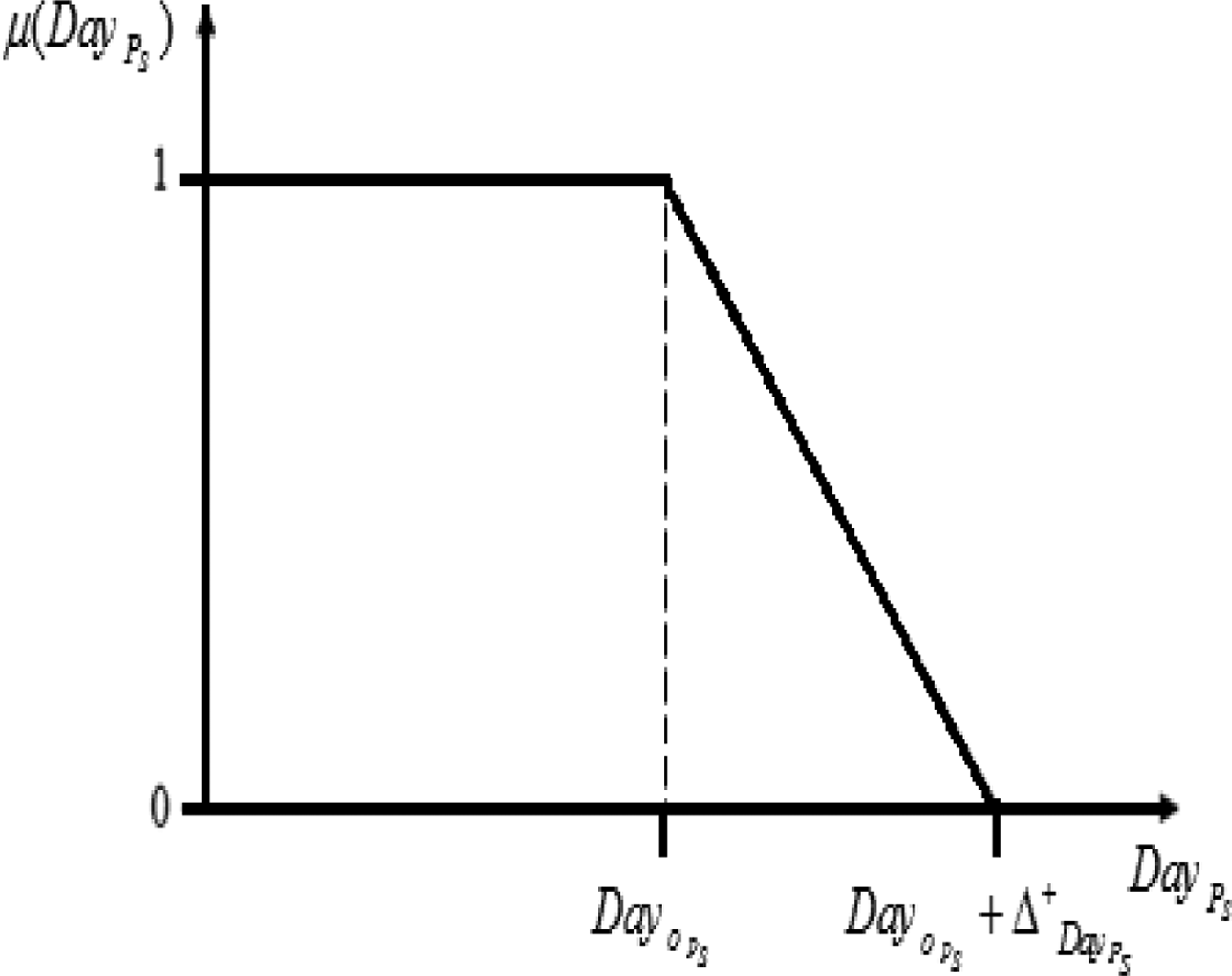
; thus, the STB function is shown in Figure 2. The objective function is to maximize total patients' satisfaction. Mathematically (19),
 $${\rm Max}\sum\limits_{P_S = 1}^{P_S} {{\rm \mu} ({\rm Da}{\rm y}_{P_S})}. $$
Smaller-the-better function.

The constraints of the model are as follows: let
 ${\rm \delta} _{{\rm Da}{\rm y}_{P_S}}^ + $
denote any positive deviation from the target value (
 ${\rm Da}{\rm y}_{o_{P_S}}$
), where its value is always positive and less than the maximum permitted positive deviation as expressed in inequality (20).
 $$0 \le {\rm \delta} _{{\rm Da}{\rm y}_{P_S}}^ + \le \Delta _{{\rm Da}{\rm y}_{P_S}}^ +\comma \, \quad \forall p_S.$$
The amount of the positive deviation from the target value is determined using Eq. (21)
 $${\rm Da}{\rm y}_{\,p_S} - {\rm \delta} _\;{{\rm Day}_{\,p_S}}^ + \le {\rm Da}{\rm y}_{o_{\,p_S}}\comma \,\quad \forall p_S.$$
Equation (22) is used to calculate the value of the membership function.
 $${\rm \mu} ({\rm Da}{\rm y}_{\,p_S}) + \displaystyle{{{\rm \delta} _{{\rm Da}{\rm y}_{\,p_S}}^ +} \over {\Delta _{{\rm Da}{\rm y}_{\,p_S}}^ +}} = 1\comma \,\quad \forall p_S.$$
Where patient satisfaction should always be higher than the minimum patient satisfaction (θ p ); or mathematically (23):
 $${\rm \mu} ({\rm Da}{\rm y}_{\,p_S}) \ge {\rm \theta} _p\comma \,\quad \forall p_S.$$
Case 3: The larger-the-better (LTB) type satisfaction
Let p
L
denote a patient's index and
 ${\rm Da}{\rm y}_{P_L}$
denote his or her scheduled date. The goal of this submodel is to maximize patients' satisfaction for patients who need to be assigned after a specific preferable date where their satisfaction will be 100% if they are assigned after that date (
 ${\rm Da}{\rm y}_{o_{\,p_L}}$
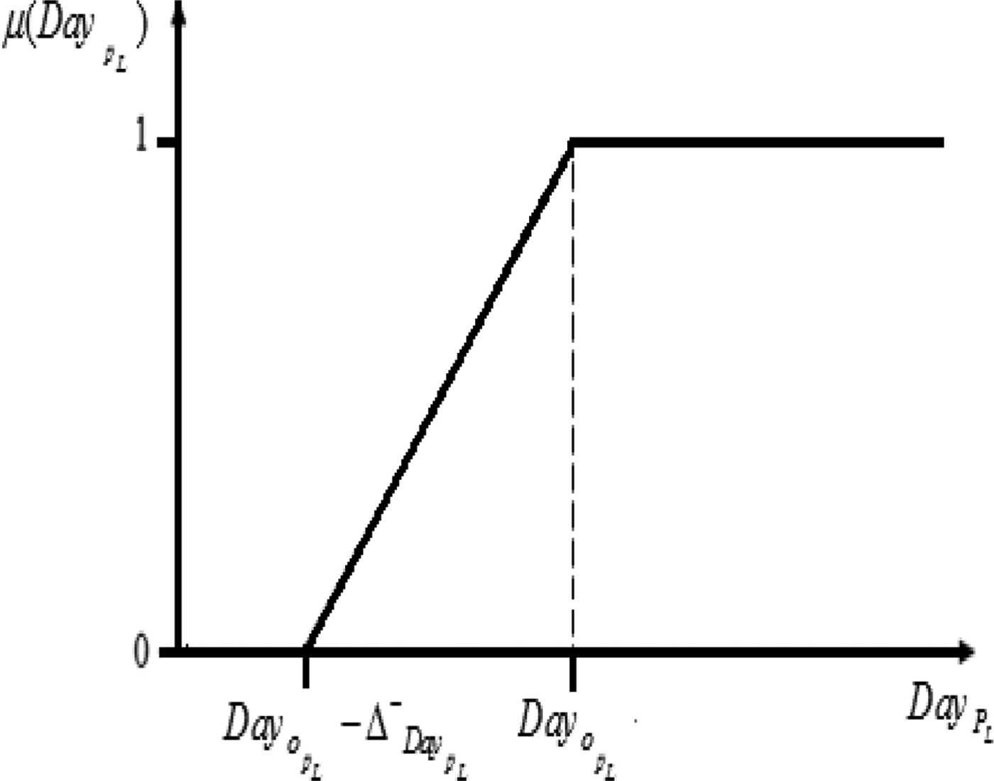
). The suitable membership function is the LTB type shown in Figure 3. Let
 ${\rm \mu} \lpar {{\rm Da}{\rm y}_{\,p_L}} \rpar $
denotes the membership function of a patient's satisfaction about his/her assigned date and
 $\Delta _{{\rm Da}{\rm y}_{\,pL}}^ - $
denote the maximum negative allowed deviation from
 ${\rm Da}{\rm y}_{o_{\,p_L}}$
. The objective function is to maximize patients' satisfaction. That is (24),
 $${\rm Max}\sum\limits_{\,p_L = 1}^{P_L} {{\rm \mu} ({\rm Da}{\rm y}_{\,p_L})}. $$
Larger-the-better function.

The constraints are developed as follows. Let
 ${\rm \delta} _{{\rm Da}{\rm y}_{\,p_N}}^ - $
denote the negative deviation from the target value (
 ${\rm Da}{\rm y}_{o_{\,p_L}}$
). It is obvious that the value of any negative deviation should be always positive and less than the maximum permitted negative deviation, that is (25),
 $$0 \le {\rm \delta} _{{\rm Da}{\rm y}_{\,p_L}}^ - \le \Delta _{{\rm Da}{\rm y}_{P_L}}^ -\comma \, \quad \forall p_L$$
The value of the negative deviation is calculated using Equation (26):
 $${\rm Da}{\rm y}_{\,p_L} + {\rm \delta} _{{\rm Da}{\rm y}_{\,p_L}}^ - = {\rm Da}{\rm y}_{o_{\,p_L}}\comma \,\quad \forall p_L$$
The value of the membership function is calculated as (27):
 $${\rm \mu} ({\rm Da}{\rm y}_{\,p_L}) + \displaystyle{{{\rm \delta} _{{\rm Da}{\rm y}_{\,p_L}}^ -} \over {\Delta _{{\rm Da}{\rm y}_{\,p_L}}^ -}} = 1\comma \,\quad \forall p_L$$
The value of each patient satisfaction should not be less than the minimum patient satisfaction denoted by θ p , which is expressed as in Eq. (28):
 $${\rm \mu} ({\rm Da}{\rm y}_{\,p_L}) \ge {\rm \theta} _p\comma \,\quad \forall p_L$$
The complete scheduling model aims at minimizing overtime, undertime, and maximizing their satisfaction concurrently through combining formulas (1) to (28).
2.1.3. Scheduling optimization model
Combining the developed objectives with their associated constraints, the complete model for optimal scheduling is formulated as follows:
 $${\rm Min}\sum\limits_{t = 1}^T {\sum\limits_{r = 1}^R {{\rm O}{\rm T}_{rt}}} + \sum\limits_{t = 1}^T {\sum\limits_{r = 1}^R {{\rm U}{\rm T}_{rt}}} $$
objective function (1) in 2.1.1,
 $${\rm Max}\sum\limits_{\,p_N = 1}^{P_N} {{\rm \mu} ({\rm Da}{\rm y}_{P_N})} + \sum\limits_{\,p_s = 1}^{P_S} {{\rm \mu} ({\rm Da}{\rm y}_{PS})} + \sum\limits_{\,p_L = 1}^{P_L} {{\rm \mu} ({\rm Da}{\rm y}_{\,p_L})} $$
objective functions (13), (19), and (24) in 2.1.2, subject to
 $${\rm O}{\rm T}_{rt} \ge {\rm \lambda} _{rt}\left( {\sum\limits_{\,p = 1}^P {{\rm \xi}_{\,prt} \times Tsur_p - {\rm \alpha}_{rt}}} \right)\comma \,\quad \forall r\comma \,t$$
[overtime] inequality (2) in 2.1.1,
 $${\rm O}{\rm T}_{rt} \ge 0\comma \,\quad \forall r\comma \,t$$
[overtime positivity] inequality (4) in 2.1.1,
 $${\rm U}{\rm T}_{rt} \ge {\rm \lambda} _{rt}\left( {{\rm \alpha}_{rt} - \sum\limits_{\,p = 1}^P {{\rm \xi}_{\,prt} \times Tsur_p}} \right)\comma \,\quad \forall r\comma \,t$$
[undertime] inequality (3) in 2.1.1,
 $${\rm U}{\rm T}_{rt} \ge 0\comma \,\quad \forall r\comma \,t$$
[undertime positivity] inequality (5) in 2.1.1,
 $$\sum\limits_{\,p = 1}^P {({\rm \xi} _{\,prt} \times Tsur_p)} - {\rm \alpha} _{rt} \le O_{rt}\comma \,\quad \forall r\comma \,t$$
[OR availability] inequality (6) in 2.1.1,
 $$\sum\limits_{\,p = 1}^P {\sum\limits_{r = 1}^R {{\rm \xi} _{\,prt} \times Tsur_p}} \times {\rm \beta} _{\,ps} \times {\rm \zeta} _{st} \le C_{st}\comma \,\quad \forall s\comma \,t$$
[surgeon availability] inequality (7) in 2.1.1,
 $${\rm \xi} _{\,prt} \le {\rm \lambda} _{rt} \times {\rm \eta} _{\,prt} \times \sum\limits_{s = 1}^S {({\rm \beta} _{\,ps} \times {\rm \zeta} _{st})\comma \,\quad \forall r\comma \,p\comma \,t} $$
[equipment availability] inequality (8) in 2.1.1,
 $$\sum\limits_{t = 1}^{{\rm Du}{\rm e}_p} {\sum\limits_{r = 1}^R {{\rm \xi} _{\,prt} \le 1}\comma \, \quad \forall p} $$
[assignment before or on due date] inequality (9) in 2.1.1,
 $$\sum\limits_{t = 1}^{{\rm Hos}_p - 1} {\sum\limits_{r = 1}^R {{\rm \xi} _{\,prt} = 0}\comma \, \quad \forall p} \in [1\comma \,.\,.\,.\,\comma \,P]/{\rm Hos}_p \gt 1$$
[patient's availability] Eq. (10) in 2.1.1,
 $${\rm Da}{\rm y}_p = \sum\limits_{t = 1}^T {\sum\limits_{r = 1}^R {(t \times {\rm \xi} _{\,prt}) + M} \times \left( {1 - \sum\limits_{t = 1}^T {\sum\limits_{r = 1}^R {(t \times {\rm \xi}_{\,prt})}}} \right)\comma \,\quad \forall p} $$
[patient's assigned date] Eq. (11) in 2.1.1,
 $${\rm \xi} _{\,prt} \in \{ 0\comma \,1\}. $$
[binary variable] Eq. (12) in 2.1.1,
 $$0 \le \delta _{{\rm Da}{\rm y}_{P_N}}^ + \le \Delta _{{\rm Da}{\rm y}_{P_N}}^ +\comma \, \quad \forall p_N$$
[positive deviation range for NTB] inequality (14) in 2.1.2,
 $$0 \le {\rm \delta} _{{\rm Da}{\rm y}_{P_N}}^ - \le \Delta _{{\rm Da}{\rm y}_{P_N}}^ -\comma \, \quad \forall p_N$$
[negative deviation range for NTB] inequality (15) in 2.1.2,
 $${\rm Da}{\rm y}_{P_N} + {\rm \delta} _{{\rm Da}{\rm y}_{P_N}}^ - + {\rm \delta} _{{\rm Da}{\rm y}_{P_N}}^ + = {\rm Da}{\rm y}_{o_{P_N}}\comma \,\quad \forall p_N$$
[deviations value for NTB] Eq. (16) in 2.1.2,
 $${\rm \mu} \lpar {{\rm Da}{\rm y}_{P_N}} \rpar + \displaystyle{{{\rm \delta} _{{\rm Da}{\rm y}_{P_N}}^ -} \over {\Delta _{{\rm Da}{\rm y}_{P_N}}^ -}} + \displaystyle{{{\rm \delta} _{{\rm Da}{\rm y}_{P_N}}^ +} \over {\Delta _{{\rm Da}{\rm y}_{P_N}}^ +}} = 1\comma \,\quad \forall p_N$$
[satisfaction value for NTB] Eq. (17) in 2.1.2,
 $${\rm \mu} \lpar {{\rm Da}{\rm y}_{P_N}} \rpar \ge \theta _p\comma \,\quad \forall p_N$$
[minimum satisfaction for NTB] inequality (18) in 2.1.2,
 $$0 \le {\rm \delta} _{{\rm Da}{\rm y}_{P_S}}^ + \le \Delta _{{\rm Da}{\rm y}_{P_S}}^ +\comma \, \quad \forall p_S$$
[positive deviation range for STB] inequality (20) in 2.1.2,
 $${\rm Da}{\rm y}_{\,p_S} - \delta _{{\rm Da}{\rm y}_{\,p_S}}^ + \le {\rm Da}{\rm y}_{o_{\,p_S}}\comma \,\quad \forall p_S$$
[deviation value for STB] inequality (21) in 2.1.2,
 $${\rm \mu} ({\rm Da}{\rm y}_{\,p_S}) + \displaystyle{{\delta _{{\rm Da}{\rm y}_{\,p_S}}^ +} \over {\Delta _{{\rm Da}{\rm y}_{\,p_S}}^ +}} = 1\comma \,\quad \forall p_S$$
[satisfaction value for STB] Eq. (22) in 2.1.2,
 $${\rm \mu} ({\rm Da}{\rm y}_{\,p_S}) \ge {\rm \theta} _p\comma \,\quad \forall p_S$$
[minimum satisfaction for STB] inequality (23) in 2.1.2,
 $$0 \le {\rm \delta} _{{\rm Da}{\rm y}_{\,p_L}}^ - \le \Delta _{{\rm Da}{\rm y}_{P_L}}^ -\comma \, \quad \forall p_L$$
[negative deviation range for LTB] inequality (25) in 2.1.2,
 $${\rm Da}{\rm y}_{\,p_L} + {\rm \delta} _{{\rm Da}{\rm y}_{\,p_L}}^ - = {\rm Da}{\rm y}_{o_{\,p_L}}\comma \,\quad \forall p_L$$
[deviation value for LTB] Eq. (26) in 2.1.2,
 $${\rm \mu} ({\rm Da}{\rm y}_{\,p_L}) + \displaystyle{{{\rm \delta} _{{\rm Da}{\rm y}_{\,p_L}}^ -} \over {\Delta _{{\rm Da}{\rm y}_{\,p_L}}^ -}} = 1\comma \,\quad \forall p_L$$
[satisfaction value for LTB] Eq. (27) in 2.1.2,
 $${\rm \mu} ({\rm Da}{\rm y}_{\,p_L}) \ge {\rm \theta} _p\comma \,\quad \forall p_L$$
[minimum satisfaction for LTB] inequality (28) in 2.1.2.
2.2. Model I: Optimization model for OR sequencing
The goal of this model is to identify the start times for each patient surgery while ensuring that the partent's satisfaction is met. It is assumed that the time durations are deterministic and should be considered during OR sequencing, and normal room working time is 420 min, and the maximum overtime allowed is 60 min. Then, the sequencing optimization model considers different objective functions. These objectives with the associated constraints are formulated as follows.
2.2.1. Minimizing total overtime
Let the intermediate variables U rt and OT rt denote the closing time and overtime of room r at day t, respectively. The objective function is to minimize the total overtime of all the rooms over the scheduling period. Mathematically (29);
 $${\rm Min}\sum\limits_{t = 1}^T {\sum\limits_{r = 1}^R {{\rm O}{\rm T}_{rt}}}. $$
The associated constraints are formulated as follows:
-
1. The summation of the required time for each patient in the OR identifies its closing time. Therefore, the closing time of room r on day t is larger than or equal to the summation of the surgery start time, st p , the time needed for preparation, set p , the duration of surgery itself, opn p , and cleaning time, cl p , for each patient treated in that room on that day. That is (30),
(30)
$$\eqalign{ U_{rt} \ge st_p + set_p + opn_p + cl_p - M(1 - {\rm \xi} _{\,prt})\comma & \cr &\forall p\comma \,r\comma \,t.}$$
-
2. Overtime for each OR on each day is larger than or equal to its working time. Let On t denote the opening time of hospital on day t. Then, the overtime of room r on day t is the difference between the closing time and regular opening time, as expressed in inequality (31):
(31)and
$${\rm O}{\rm T}_{rt} \ge U_{rt} - ({\rm \alpha} _{rt} - On_t)\comma \,\quad \forall r\comma \,t$$
(32)
$${\rm O}{\rm T}_{rt} \ge 0\comma \,\quad \forall r\comma \,t.$$
-
3. Overtime for each day and each room should be less than the maximum overtime availability as presented in Eq. (33):
(33)
$${\rm O}{\rm T}_{rt} \le O_{rt}\comma \,\quad \forall r\comma \,t.$$
-
4. All surgeries should start after the opening time of the hospital as expressed in inequality (34):
(34)
$$st_p \ge On_t\comma \,\quad \forall p\comma \,t.$$
-
5. Surgeons should operate during their working time. Let x st and z st denote the start and end of the working time of surgeon s on day t, respectively. Surgery carried out by surgeon s for patient p on day t should be completed before the end of his working time. Mathematically (35),
(35)
$$\eqalign{st_p + set_p + opn_p - M\left( {2 - {\rm \beta}_{\,ps} - \sum\limits_{r = 1}^R {{\rm \xi}_{\,prt}}} \right) \le & z_{st}\comma \cr & \forall p\comma \,s\comma \,t.}$$
-
6. The surgery for patient p treated by surgeon s should start after the surgeon working time as expressed in inequality (36).
(36)
$$\eqalign{ st_p + set_p \ge {\rm \beta} _{\,ps} \times x_{st} - M \left( 1 - \sum\limits_{r = 1}^R {{\rm \xi}_{\,prt}} \right)\comma & \cr & \quad \forall p\comma \,s\comma \,t.}$$
-
7. Each surgeon should treat one patient at a time. When patients p and j are assigned to the same surgeon such that patient j is treated after patient p, the setup for patient j should be completed after finishing the surgery of patient p, that is (37):
(37)
$$\eqalign{ st_j + & set_j \ge (st_p + set_p + opn_p) \cr &- M\left( {5 - \nu_{\,pjt} - {\rm \beta}_{\,ps} - {\rm \beta}_{\,js} - \sum\limits_{r = 1}^R {{\rm \xi}_{\,prt}} - \sum\limits_{r = 1}^R {{\rm \xi}_{\,jrt}}} \right) \cr & \qquad\qquad\qquad\qquad \forall s\comma\; t\comma\; p\comma\; j \in [1\comma \,.\,.\,.\, \comma \,P]/p \ne j.}$$
-
8. One patient should be treated in each OR in each time. When patient p is treated before patient j in room r, the start time of patient j should be greater than the whole time required for the surgery of patient p. The whole time required for patient p includes the setup time, surgery duration, and cleaning time as formulated by constraint (38).
(38)
$$\eqalign{ st_j \ge st_p + set_p + opn_p &+ cl_p - M(3 - \nu _{\,pjt} - {\rm \xi} _{\,prt} - {\rm \xi} _{\,jrt})\comma \, \cr & \forall r\comma \,t\comma \,p\comma \,j \in [1\comma \,.\,.\,.\,\comma \,P]/p \ne j.}$$
-
9. When the surgery of patient p starts before the surgery of patient j, the start time of patient j should be larger than the start time of patient p as follows (39):
(39)where v pjt is a binary variable, or (40):
$$st_j \ge st_p - M(1 - \nu _{\,pjt})\comma \,\quad \forall t\comma \,p\comma \,j \in [1\comma \,.\,.\,.\,\comma \,P]/p \ne j.$$
(40)
$$\nu _{\,pjt} \in \{ 0\comma \,1\}. $$
-
10. Surgery precedence is determined between patients treated on the same day, as presented in Eq. (41).
(41)
$$\nu _{\,pjt} + \nu _{\,jpt} = \sum\limits_{r = 1}^R {{\rm \xi} _{\,prt}} \times \sum\limits_{r = 1}^R {{\rm \xi} _{\,jrt}}\comma \, \quad \forall t\comma \,p\comma \,j \in [1\comma \,.\,.\,.\,\comma \,P]/p \gt j.$$


2.2.2. Maximizing patient's satisfaction
Case 1: Trapezoidal satisfaction membership function
The goal of this submodel is to maximize patients' satisfaction for patients, who have a preferable period of time to start their surgery. Let p
N
denote patient's index and
 $st_{\,p_N}$
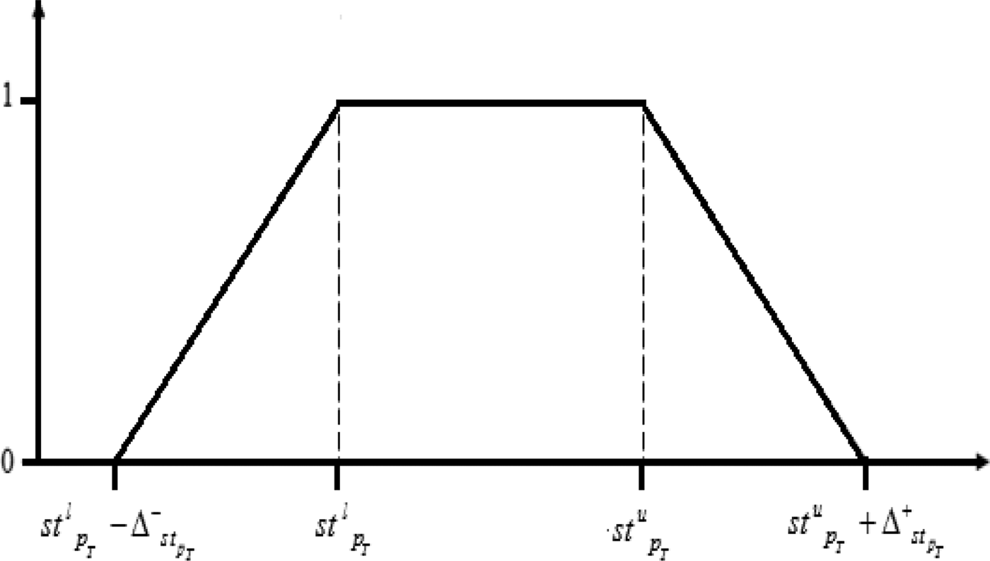
denote start time. If patient's surgery starts in his/her preferable period of time, the satisfaction will be 100%. Trapezoidal shown in Figure 4 is the proper membership function that presents a patient's satisfaction about his/her start time,
 ${\rm \mu} \lpar {st_{\,p_T}} \rpar $
. Let the upper and lower limits of the preferable period of time be denoted by
 $st_{\,p_T}^u $
and
 $st_{\,p_T}^l $
, respectively. Let
 $\Delta _{st_{\,pT}}^ - $
and
 $\Delta _{st_{\,pT}}^ + $
denote the maximum negative and positive allowable deviation from
 $st_{\,p_T}^l $
.
Trapezoidal patient satisfaction function

The objective function is to maximize patients' satisfaction, which is formulated as follows (42):
 $${\rm Max}\sum\limits_{\,p_T = 1}^{P_T} {{\rm \mu} (st_{\,p_T})}. $$
The model constraints are set as follows. Let
 ${\rm \delta} _{st_{\,pT}}^ + $
denotes any positive deviation from the upper limit of the preferable period of time,
 $st_{\,p_T}^u $
, and
 ${\rm \delta} _{st_{\,pT}}^ - $
denotes any negative deviation from the lower limit of the preferable period of time,
 $st_{\,p_T}^l $
. Then (43) and (44),
 $$0 \le {\rm \delta} _{st_{\,p_T}}^ + \le \Delta _{st_{\,p_T}}^ +\comma \, \quad \forall p_T.$$
 $$0 \le {\rm \delta} _{st_{p_T}}^ - \le \Delta _{st_{p_T}}^ -\comma \, \quad \forall p_T.$$
The amount of any negative deviation is how far the start time is from the lower limit. That is (45),
 $$st_{\,p_T} + {\rm \delta} _{st_{\,p_T}}^ - \ge st_{\,p_T}^l\comma \, \quad \forall p_T.$$
The amount of any positive deviation is determined by start time distant from the upper limit. Mathematically (46),
 $$st_{\,p_T} - {\rm \delta} _{st_{\,p_T}}^ + \le st_{\,p_T}^u\comma \, \quad \forall p_T.$$
Further, the value of the membership function is calculated using Eq. (47).
 $${\rm \mu} \lpar {st_{\,p_T}} \rpar + \displaystyle{{{\rm \delta} _{st_{\,p_T}}^ -} \over {\Delta _{st_{\,p_T}}^ -}} + \displaystyle{{{\rm \delta} _{st_{\,p_T}}^ +} \over {\Delta _{st_{\,p_T}}^ +}} = 1\comma \,\quad \forall p_T.$$
Finally, the value of each patient satisfaction,
 ${\rm \mu} \lpar {st_{\,p_T}} \rpar $
, should not be less that the minimum patient satisfaction denoted by, θ
p
which is expressed as (48)
 $${\rm \mu} \lpar {st_{\,p_T}} \rpar \ge {\rm \theta} _p\comma \,\quad \forall p_T.$$
Case 2: STB satisfaction membership function
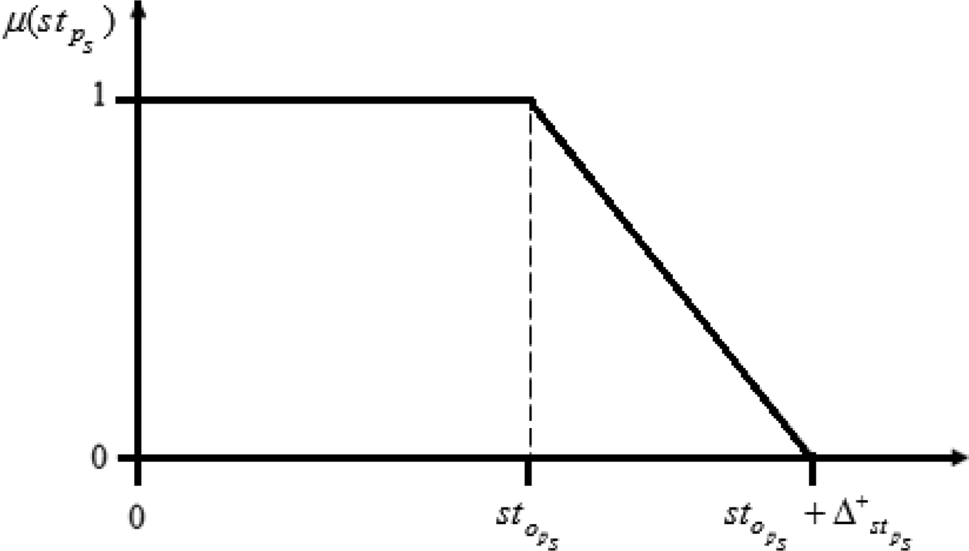
This case aims to maximize patients' satisfaction for patients who preferred to start their surgery any time during the day but before a certain time (
 $st_{o_{\,p_S}}$
); their satisfaction will decrease if they are assigned after that certain time. Thus, the proper membership function is the STB type shown in Figure 5.
Smaller-the-better patient satisfaction function.

Let
 ${\rm \mu} \lpar {st_{\,p_S}} \rpar $
denote the membership function that presents a patient's satisfaction about his/her assigned date and
 $\Delta _{st_{\,pS}}^ + $
denote the maximum positive permitted deviation from
 $st_{o_{\,p_S}}$
.
The objective function is to maximize total patients' satisfaction as follows (49):
 $${\rm Max}\sum\limits_{\,p_S = 1}^{P_S} {{\rm \mu} (st_{\,p_S})}. $$
The model constraints are built as follows. Let
 $\Delta _{st_{\,pS}}^ + $
denote any positive deviation from the latest start time (
 $st_{o_{\,p_S}}$
), where its value is always positive and less than the maximum allowed positive deviation. That is (50),
 $$0 \le {\rm \delta} _{st_{\,p_S}}^ + \le \Delta _{st_{\,pS}}^ +\comma \, \quad \forall p_S.$$
The amount of the positive deviation from the target value and the value of the membership function is identifies as inequality (51) and Eq. (52), respectively.
 $$st_{\,p_S} - {\rm \delta} _{st_{\,pS}}^ + \le st_{o_{\,p_S}}\comma \,\quad \forall p_S.$$
 $${\rm \mu} \lpar {st_{p_S}} \rpar + \displaystyle{{{\rm \delta} _{st_{p_S}}^ +} \over {\Delta _{st_{pS}}^ +}} = 1\comma \,\quad \forall p_S.$$
Further, patient satisfaction should always be higher than the minimum patient's satisfaction (θ p ), which is expressed as follows (53):
 $${\rm \mu} \lpar {st_{\,p_S}} \rpar \ge {\rm \theta} _p\comma \,\quad \forall p_S.$$
Case 3: LTB satisfaction membership function
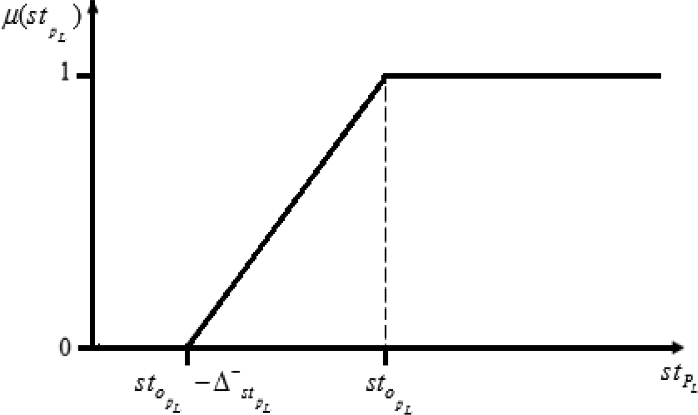
This case maximizes patients' satisfaction for patients who need to be treated at any time but after a specific time (
 $st_{o_{\,p_L}}$
), where their satisfaction will be 100% if they are assigned after that specific time. Thus, the proper membership function is LTB as shown in Figure 6. Let
 ${\rm \mu} \lpar {st_{\,p_L}} \rpar $
denote the membership function, which represents a patient's satisfaction about his/her scheduled start time. In addition, let
 $\Delta _{st_{\,pL}}^ - $
denote the maximum negative allowable deviation from
 $st_{o_{\,p_L}}$
.
The objective function is to maximize patients' satisfaction, which is formulated as follows (54):
 $${\rm Max}\sum\limits_{\,p_L = 1}^{P_L} {{\rm \mu} (st_{\,p_L})}. $$
Larger-the-better patient satisfaction function.

The model constraints are developed as follows. Let
 $\delta _{st_{\,pN}}^ - $
denote the negative deviation from the earliest preferable start time (
 $st_{o_{\,p_L}}$
). Then, any negative deviation should be always positive and less than the maximum permitted negative deviation, which is formulated as (55):
 $$0 \le {\rm \delta} _{st_{\,p_L}}^ - \le \Delta _{st_{\,pL}}^ -\comma \, \quad \forall p_L.$$
The value of the negative deviation is calculated using (56)
 $$st_{\,p_L} + {\rm \delta} _{st_{\,pL}}^ - = st_{o_{\,p_L}}\comma \,\quad \forall p_L.$$
The value of the membership function is given by (57)
 $${\rm \mu} \lpar {st_{\,pL}} \rpar + \displaystyle{{{\rm \delta} _{st_{\,p_L}}^ -} \over {\Delta _{st_{\,pL}}^ -}} = 1\comma \,\quad \forall p_L$$
The value of each patient satisfaction should not be less than the minimum patient satisfaction denoted by θ p , which is expressed as (58)
 $${\rm \mu} \lpar {st_{\,p_L}} \rpar \ge {\rm \theta} _p\comma \,\quad \forall p_L.$$
2.3. Model II: Sequencing optimization model
The developed objectives and their associated constraints are combined into a complete sequencing model, which is written as follows:
 $${\rm Min}\sum\limits_{t = 1}^T {\sum\limits_{r = 1}^R {{\rm O}{\rm T}_{rt}}} $$
objective function (29) in 2.2.1,
 $${\rm Max}\sum\limits_{\,p_T = 1}^{P_T} {{\rm \mu} (st_{\,p_T})} + \sum\limits_{\,p_s = 1}^{P_S} {{\rm \mu} (st_{\,pS})} + \sum\limits_{\,p_L = 1}^{P_L} {{\rm \mu} (st_{\,p_L})} $$
objective function (42), (49), and (54) in 2.2.2, subject to
 $$U_{rt} \ge st_p + set_p + opn_p + cl_p - M(1 - {\rm \xi} _{\,prt})\comma \,\quad \forall p\comma \,r\comma \,t$$
[closing time] inequality (30) in 2.2.1,
 $${\rm O}{\rm T}_{rt} \ge U_{rt} - ({\rm \alpha} _{rt} - On_t)\comma \,\quad \forall r\comma \,t$$
[overtime] inequality (31) in 2.2.1,
 $${\rm O}{\rm T}_{rt} \ge 0\comma \,\quad \forall r\comma \,t$$
[overtime positivity] inequality (32) in 2.2.1,
 $${\rm O}{\rm T}_{rt} \le O_{rt}\comma \,\quad \forall r\comma \,t\comma \,$$
[limiting overtime] inequality (33) in 2.2.1,
 $$st_p \ge On_t\comma \,\quad \forall p\comma \,t$$
[surgeries to start after hospital's opening] inequality (34) in 2.2.1,
 $$\eqalign{ st_p + set_p + opn_p - M\left( {2 - {\rm \beta}_{\,ps} - \sum\limits_{r = 1}^R {{\rm \xi}_{\,prt}}} \right) \le z_{st}\comma \,\quad \forall p\comma \,s\comma \,t} $$
[surgeries to be within surgeon working time] inequality (35) in 2.2.1,
 $$st_p + set_p \ge {\rm \beta} _{\,ps} \times x_{st} - M\left( {1 - \sum\limits_{r = 1}^R {{\rm \xi}_{\,prt}}} \right)\comma \,\quad \forall p\comma \,s\comma \,t$$
[surgeries to be within surgeon working time] inequality (36) in 2.2.1,
 $$\eqalign{ st_j + set_j &\ge (st_p + set_p + opn_p) \cr & M\left( {5 - \nu_{\,pjt} - {\rm \beta}_{\,ps} - {\rm \beta}_{\,js} - \sum\limits_{r = 1}^R {{\rm \xi}_{\,prt}} - \sum\limits_{r = 1}^R {{\rm \xi}_{\,jrt}}} \right) \cr & \qquad\qquad\qquad\qquad\qquad\qquad \forall s\comma \,t\comma \,p\comma \,j \in [1\comma \,.\,.\,.\,\comma \,P]/p \ne j} $$
[surgeon performs one surgery at a time] inequality (37) in 2.2.1,
 $$\eqalign{ st_j \ge st_p + set_p + opn_p + cl_p - M(3 - &\nu _{\,pjt} - {\rm \xi} _{\,prt} - {\rm \xi} _{\,jrt})\comma \, \cr & \forall r\comma \,t\comma \,p\comma \,j \in [1\comma \,.\,.\,.\,\comma \,P]/p \ne j} $$
[OR occupied by one patient at a time] inequality (38) in 2.2.1,
 $$st_j \ge st_p - M(1 - \nu _{\,pjt})\comma \,\quad \forall t\comma \,p\comma \,j \in [1\comma \,.\,.\,.\,\comma \,P]/p \ne j$$
[respecting patient precedence in OR] inequality (39) in 2.2.1,
 $$\nu _{{\kern 1pt} pjt} + \nu _{{\kern 1pt} jpt} = \sum\limits_{r = 1}^R {\xi _{{\kern 1pt} prt}} \times \sum\limits_{r = 1}^R {\xi _{{\kern 1pt} jrt}} ,\quad \forall t,{\mkern 1mu} p,{\mkern 1mu} j \in [1,{\mkern 1mu} .{\mkern 1mu} .{\mkern 1mu} .{\mkern 1mu} ,{\mkern 1mu} P]/p \gt j$$
[surgery precedence] Eq. (41) in 2.2.1,
 $$\nu _{\,pjt} \in \lcub0\comma \,1\rcub. $$
[binary variables] Eq. (40) in 2.2.1,
 $$0 \le {\rm \delta} _{st_{\,p_T}}^ + \le \Delta _{st_{\,p_T}}^ +\comma \, \quad \forall p_T$$
[positive deviation range for trapezoidal] inequality (42) in 2.2.2,
 $$0 \le {\rm \delta} _{st_{\,p_T}}^ - \le \Delta _{st_{\,p_T}}^ -\comma \, \quad \forall p_T$$
[negative deviation range for trapezoidal] inequality (43) in 2.2.2,
 $$st_{\,p_T} + {\rm \delta} _{st_{\,p_T}}^ - \ge st_{\,p_T}^u\comma \, \quad \forall p_T$$
[negative deviation value for trapezoidal] inequality (45) in 2.2.2,
 $$st_{\,p_T} - {\rm \delta} _{st_{\,p_T}}^ + \le st_{\,p_T}^u\comma \, \quad \forall p_T$$
[positive deviation value for trapezoidal] inequality (46) in 2.2.2.
 $${\rm \mu} \lpar {st_{\,p_T}} \rpar + \displaystyle{{{\rm \delta} _{st_{\,p_T}}^ -} \over {\Delta _{st_{\,p_T}}^ -}} + \displaystyle{{{\rm \delta} _{st_{\,p_T}}^ +} \over {\Delta _{st_{\,p_T}}^ +}} = 1\comma \,\quad \forall p_T$$
[satisfaction value for trapezoidal] Eq. (47) in 2.2.2,
 $${\rm \mu} \lpar {st_{\,p_T}} \rpar \ge {\rm \theta} _p\comma \,\quad \forall p_T$$
[minimum satisfaction for trapezoidal] inequality (48) in 2.2.2,
 $$0 \le {\rm \delta} _{st_{\,p_S}}^ + \le \Delta _{st_{\,pS}}^ +\comma \, \quad \forall p_S$$
[positive deviation range for STB] inequality (50) in 2.2.2,
 $$st_{\,p_S} - {\rm \delta} _{st_{\,pS}}^ + \le st_{o_{\,p_S}}\comma \,\quad \forall p_S$$
[deviation value for STB] inequality (51) in 2.2.2,
 $${\rm \mu} \lpar {st_{\,p_S}} \rpar + \displaystyle{{{\rm \delta} _{st_{\,p_S}}^ +} \over {\Delta _{st_{\,pS}}^ +}} = 1\comma \,\quad \forall p_S$$
[satisfaction value for STB] Eq. (52) in 2.2.2,
 $${\rm \mu} \lpar {st_{\,p_S}} \rpar \ge \theta _p\comma \,\quad \forall p_S$$
[minimum satisfaction for STB] inequality (53) in 2.2.2,
 $$0 \le {\rm \delta} _{st_{\,p_L}}^ - \le \Delta _{st_{\,pL}}^ -\comma \, \quad \forall p_L$$
[negative deviation range for LTB] inequality (55) in 2.2.2,
 $$st_{\,p_L} + {\rm \delta} _{st_{\,pL}}^ - = st_{o_{\,p_L}}\comma \,\quad \forall p_L$$
[deviation value for LTB] Eq. (56) in 2.2.2,
 $${\rm \mu} \lpar {st_{\,pL}} \rpar + \displaystyle{{{\rm \delta} _{st_{\,p_L}}^ -} \over {\Delta _{st_{\,pL}}^ -}} = 1\comma \,\quad \forall p_L$$
[satisfaction value for LTB] Eq. (57) in 2.2.2,
 $${\rm \mu} \lpar {st_{\,p_L}} \rpar \ge {\rm \theta} _p\comma \,\quad \forall p_L$$
[minimum satisfaction for LTB] inequality (58) in 2.2.2.
3. ILLUSTRATIONS
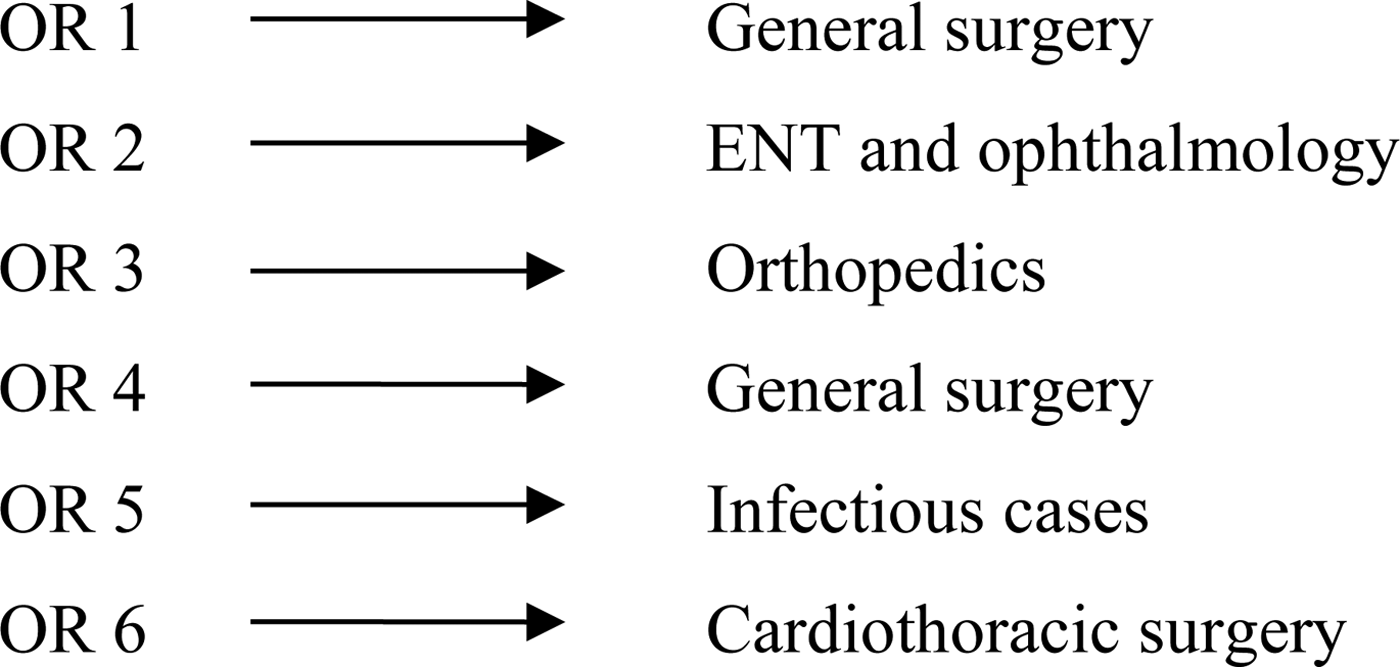
The proposed models were implemented in a hospital that provides comprehensive surgical operations for all surgical specialties. Its OR department includes six ORs, five of which contain general surgical equipment and can be used to conduct any surgical procedure, except for cardiothoracic surgery. OR6 is specially designated for cardiothoracic surgery (no other OR can be used for performing surgeries of this specialty) and can also be used for conducting surgeries of all other specialties. However, the hospital's method of OR scheduling involves assigning surgeries of particular specialties to each of the five general rooms, as shown in Figure 7.
Preferred operating room segmentation in the hospital.

3.1. Analysis of OR scheduling
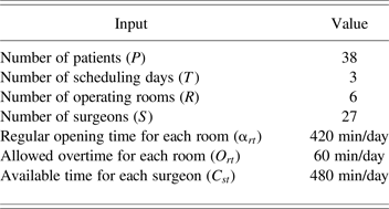
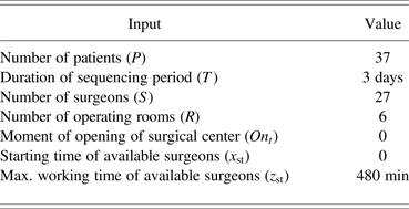
The model was implemented to schedule 38 patients over 3 days. In this hospital, there were 27 surgeons and 6 ORs. According to the labor regulations, the regular working time (α rt ) for each OR was 420 min/day, and the allowed overtime (O rt ) for each OR was 60 min/day. The available time for each surgeon (C st ) was 480min/day. General inputs are summarized in Table 1.
Summary of Model I general inputs

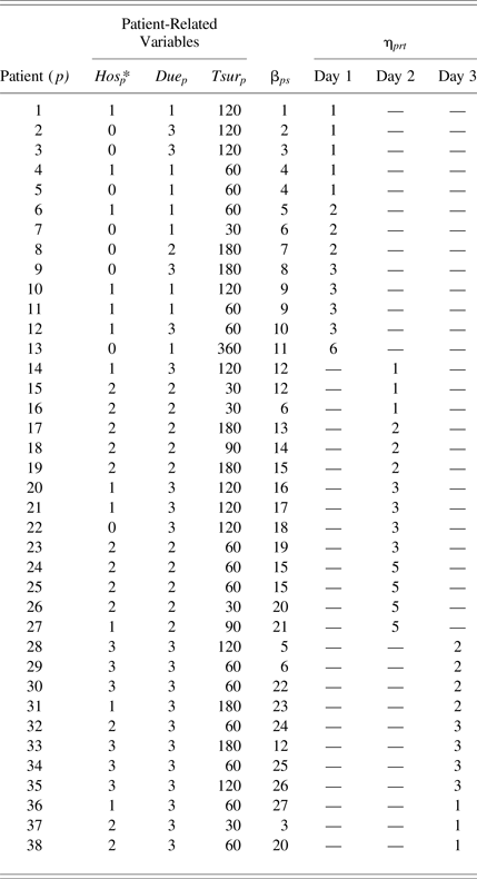
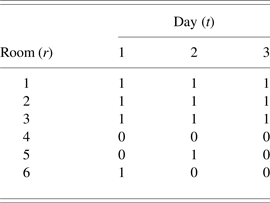
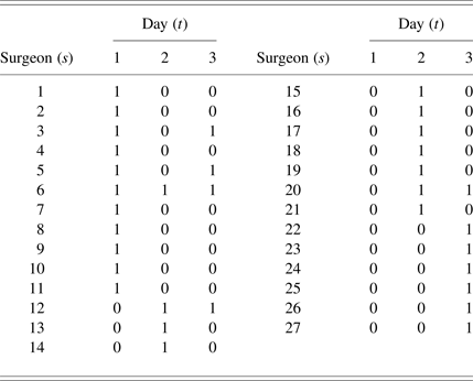
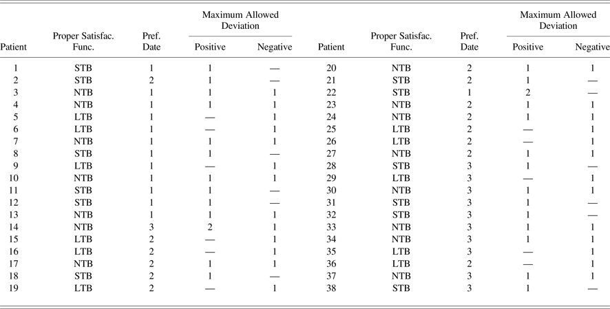
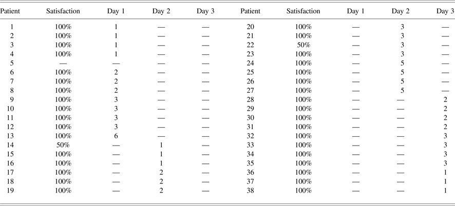
Special equipment needed for each type of surgery was distributed among hospital ORs, and each patient should be treated by a single surgeon; the distribution of equipment and surgeon assignment are shown in Table 2. The hospitalization date (Hos p ), due date (Due p ), and surgery duration (Tsur p ) for each patient are also presented in Table 2. The OR availability matrix (λ rt matrix) and surgeon availability matrix (ζ st matrix) are presented in Tables 3 and 4, respectively. The minimum accepted satisfaction for all patients is 50%. The proper satisfaction function for each patient along with his or her preferred date and the maximum allowable deviations are stated in Table 5. Using LINGO 13 software, the obtained percentage of assigned patients was 97.34%; the patient assignment matrix and their satisfaction are presented in Table 6.
Patient-related variables, βps and ηprt

Operating room availability (λrt – matrix)

Surgeons' availability (ζst – matrix)

The fuzziness information

Patients' assignment ξ prt matrix and satisfaction

3.2. Analysis of OR sequencing
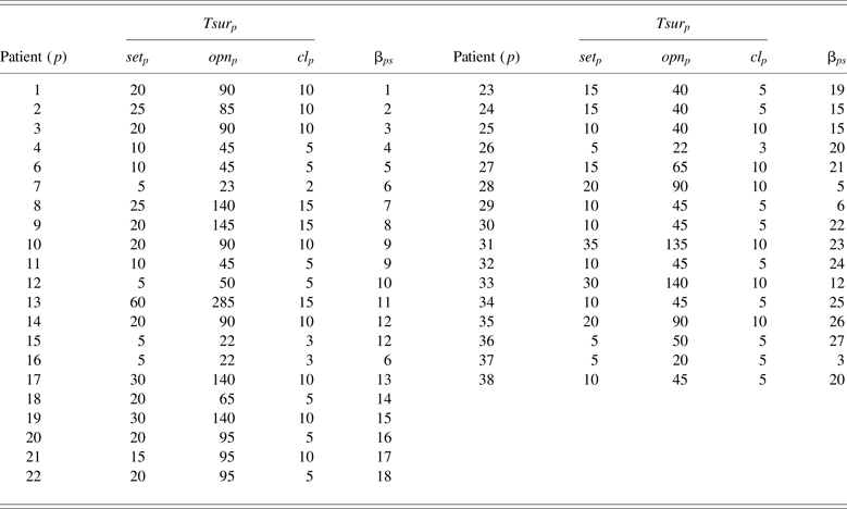
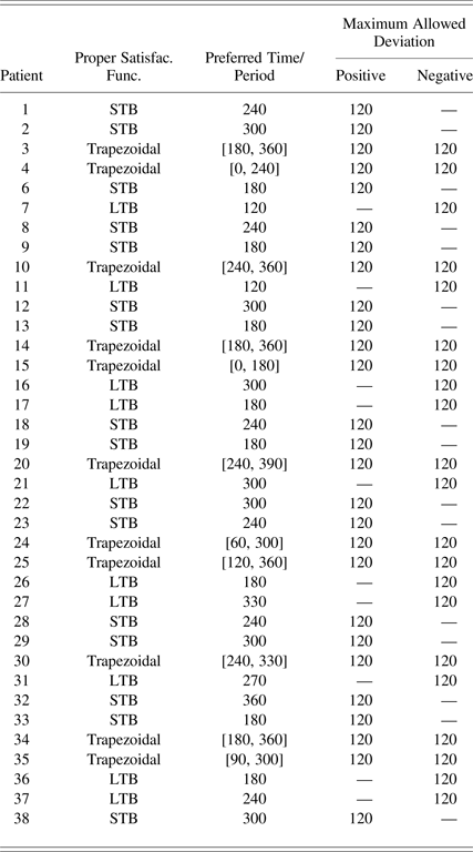
In this model, patients will be sequenced over their assigned days and rooms. Therefore, patient assignment matrix (ζ prt matrix), which was obtained in Model I, will be utilized as an input to this model. The normal working hours in ORs started from 8:00 a.m., which was considered as a time reference (Time 0). Thus, the time of the surgical center opening on all days was 0 (On t = 0). On all days, surgeons started their work (x st ) at Time 0, and their maximum working time (z st ) was 480 min [the difference between these two values was equivalent to the available working time for each surgeon (C st )]. The general inputs for Model II are summarized in Table 7. Surgery duration (Tsur p ) consisted of setup and preparation (set p ), surgical act duration (opn p ), and cleaning time (cl p ). The surgery duration components and β ps matrix are presented in Table 8. The minimum accepted satisfaction for all patients is 50%. The proper satisfaction function for each patient along with his or her preferred time and the maximum allowable deviations are stated in Table 9.
Summary of general inputs of sequencing model

Patient related durations and assigned surgeon

The fuzziness information

4. RESEARCH RESULTS
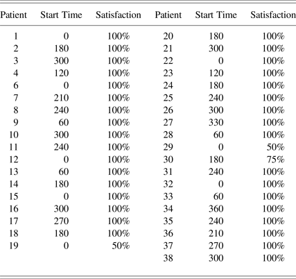
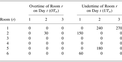
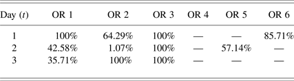
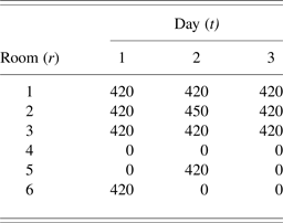
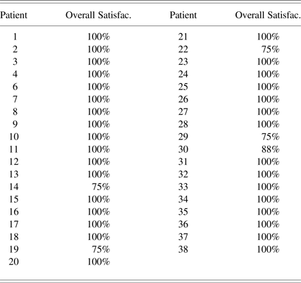
Using LINGO 13, surgery start times and patient's satisfaction were obtained and are presented in Table 10. The OR overtime and undertime (in minutes) obtained from Model I are listed in Table 11. Finally, the OR use percentages were calculated, as shown in Table 12. The overtime resulting from Model II was only 30 min scheduled for Day 2 in Room 2. The closing time for each OR is presented in Table 13. The overall patient's satisfaction is the average of the patient's satisfaction with his or her assigned day (resulted from Model I) and the patient's satisfaction with his/her scheduled time (resulted from Model II). The overall patient's satisfaction is exhibited in Table 14.
Surgeries start times and patients' satisfaction

Overtimes and undertimes of the operating rooms (min)

Operating rooms utilization

Operating rooms' closing times

The overall patient's satisfaction

5. CONCLUSIONS
Two optimization models were successfully formulated in this study for multiple-period scheduling and sequencing that takes into consideration a patient's preferred time and date for surgery. The scheduling model aimed to minimize overtime and undertime while maximizing patients satisfaction about their surgery date. After distributing patients over days and rooms, the start time of each surgery and the sequence of patients in the assigned room were determined on each day. The objective of the sequencing model is to determine the start times and sequences of patient surgeries while taking into consideration a patient's preferred time of treatment. Models were implemented on a real case in a private hospital in Jordan. The proposed optimization models can assist decision makers in improving patient satisfaction and enhancing OR utilization.
Abbas Al-Refaie is a Professor in the Department of Industrial Engineering at the University of Jordan. He is currently the Deputy Dean of the Engineering School for Academic Affairs. Prof. Al-Refaie has published more than 100 papers in reputable international journals. He also joined several international conferences. His research focuses on quality engineering, design and analysis of engineering experiments, logistics and supply chain management, optimization, healthcare, and robust design.
Mays Judeh received a Master's degree in industrial engineering from the University of Jordan. She has published several papers on optimization in healthcare applications. Her research focuses on optimization, scheduling and sequencing, and optimization.
Ming-Hsien Li is a Professor in the Department of Industrial Engineering and Systems Management at Feng Chia University. Prof. Li has published several research papers in reputable international journals. His research interests include statistical quality control, design and analysis of engineering experiments, quality management, and robust design.