

Introduction
Many populations, particularly populations of insects, show large fluctuations in abundance from one year to the next – often termed population variability or population instability. Some species show high population variability, other species relatively low variability (Lamb and MacKay Reference Lamb and MacKay2010; Lamb et al. Reference Lamb, MacKay and Alyokhin2011, Reference Lamb, MacKay and Wool2012; Galloway and Lamb Reference Galloway and Lamb2014, Reference Galloway and Lamb2015; and references therein). A number of factors are thought to influence the level of population variability. Redfearn and Pimm (Reference Redfearn and Pimm1988) hypothesise that polyphagous herbivores have lower population variability than specialist herbivores. Insect herbivores that live in monocultures may have higher population variability than those living on hosts with more natural spatial distributions (Dalin et al. Reference Dalin, Kindvall and Björkman2009; Lamb and MacKay Reference Lamb and MacKay2010). Some native aphid species exhibit lower population variability than introduced ones (Lamb and MacKay Reference Lamb and MacKay2010; Lamb et al. Reference Lamb, MacKay and Alyokhin2011, Reference Lamb, MacKay and Wool2012), and some bird lice that are abundant have lower population variability than less abundant ones (Galloway and Lamb Reference Galloway and Lamb2014). So far the number of populations available for comparison is small, and few such hypotheses have been tested rigorously.
The development and testing of hypotheses about population variability were slowed by a lack of an effective metric. Initially, standard deviation of log abundance was used (e.g., Cappuccino Reference Cappuccino1987), eventually to be replaced by the coefficient of variation of log abundance when it was recognised that standard deviation usually increases with the mean (McArdle et al. Reference McArdle, Gaston and Lawton1990). More recently Heath (Reference Heath2006) proposed a new metric for population variability, PV: the average of the differences for all pairs of abundance in a time series, with each difference divided by the larger abundance in the pair (when both members of a pair are 0, the quotient is 0). The parameter PV is a proportion ranging between 0 and 1: a perfectly stable population has a PV of 0, one that fluctuates between two extremes approaches a PV of 1. The parameter PV does not depend on log transformation, with the attendant problem of 0-values, and the temporal sequence of annual abundance in a time series does not affect the estimate of PV (Heath Reference Heath2006). The parameter PV is effective for summarising in one number a frequency distribution of annual abundances, and can be used for many types of theoretical distribution (Heath Reference Heath2006). Thus, PV is a potentially valuable metric for population variability, and for comparing this aspect of population dynamics among populations and species.
Although some statistical properties of PV have been investigated for theoretical distributions (Heath Reference Heath2006), the properties of the metric when applied to frequency distributions of annual abundance of organisms are only beginning to be understood. One property that has been investigated is the uniformity of PV when annual abundance is measured at different times during the season. Three aphid species that have different seasonal patterns of abundance all have uniform values of PV as their populations grow and decline (Lamb et al. Reference Lamb, MacKay and Alyokhin2013). These data support the use of PV for inter-specific comparisons even when there may be seasonal differences in the timing of measurement of abundance for the species under consideration. A key property of PV that has not yet been investigated is the length of the time series required to estimate PV with adequate precision to test the hypothesis at hand.
Relatively few population studies of insects have been sustained for more than a decade. This reality begs the question: how many years of data are required to effectively estimate population variability? One of the early investigations of population variability was based on a four-year comparison of two aphid species living in the same habitat (Cappuccino Reference Cappuccino1987). More recently, a seven-year study was used to compare herbivorous insect populations living on monocultures to those living on more naturally distributed hosts (Dalin et al. Reference Dalin, Kindvall and Björkman2009). Are four-year or seven-year time series sufficient for robust tests of hypotheses about population variability? A 60-year study of aphid populations revealed differences among estimates of PV values for successive five-year intervals, casting doubt on the use of short time series to estimate PV (Lamb et al. Reference Lamb, MacKay and Alyokhin2011). To reliably compare estimates of PV for different populations or for different species, an understanding of the effect of time series length on PV would be helpful.
The length of time series required to estimate PV precisely could be estimated for theoretical distributions of population abundance, although a more realistic estimate might come from actual populations if sufficiently long time series were available. The annual abundances for three aphid species on cultivated potatoes are among the longest time series measured for an insect (Alyokhin et al. Reference Alyokhin, Drummond and Sewell2005, Reference Alyokhin, Drummond, Sewell and Storch2011; Lamb et al. Reference Lamb, MacKay and Alyokhin2011). The dynamics of these populations are reasonably well understood. Two of the three aphid species show density-dependent cycles of abundance, but the third one does not (Alyokhin et al. Reference Alyokhin, Drummond and Sewell2005). Populations of the same two species decline from the beginning to the end of the time series, but the third species maintains its average abundance (Alyokhin et al. Reference Alyokhin, Drummond and Sewell2005; Lamb et al. Reference Lamb, MacKay and Alyokhin2011). The three aphids have distinct PV values of 0.59, 0.78, and 0.83 over 58 years, with two species having relatively uniform PV values from decade to decade compared with the less uniform PV of the third species (Lamb et al. Reference Lamb, MacKay and Alyokhin2011).
In the present study, we use the same data for these three aphids, with four additional years, to provide 62-year time series of annual abundance. We assess the length of time series required to make reliable estimates of PV for these three species, which exhibit different population dynamics, and different PV values. The following statistical properties were assessed for 11 time series from 3–62 years (with replication of n=20 to n=1, respectively): uniformity of mean PV, the standard deviation of PV, and the ability to correctly classify estimates of PV as higher or lower when comparing any two of the aphid species. This information should help guide future research on population variability with respect to the length of time series needed for comparing PV among populations or species.
Materials and methods
Macrosiphum euphorbiae (Thomas), Myzus persicae (Sulzer), and Aphis nasturtii (Kaltenbach) (Hemiptera: Aphididae) were counted on three potato leaves from each of 20–25 individual potato plants, from each of five or six replicate plots (15.2 m long and four rows wide) at the University of Maine Aroostook Research Farm, Presque Isle, Maine, United States of America. Potatoes were usually planted in the last two weeks of May and sampled weekly from late June to September. Counts for each species were averaged over leaves and plants to estimate abundance as the average density per leaf. Weekly data were averaged over the season to estimate annual abundance for each year from 1949 to 2013, a period of 65 years. However, data were not collected in 1965, 1968 and 1970, and in one year (2010) data were excluded for M. persicae because greenhouse-reared aphids were added to the field plots to augment populations. As a result, the time series for M. persicae is 61 years, compared with 62 years for the other two species. For convenience in the text, the time series is reported as 62 years for all three species. The plots and sampling methods are described in more detail by Alyokhin et al. (Reference Alyokhin, Drummond and Sewell2005, Reference Alyokhin, Drummond, Sewell and Storch2011) and Lamb et al. (Reference Lamb, MacKay and Alyokhin2011, Reference Lamb, MacKay and Alyokhin2013).
The frequency distributions of annual abundance for each species were assessed because we expected the shape of the distribution to affect estimates of PV and its variation. Descriptions of these distributions were also useful for assessing how relevant our conclusions are for other studies of PV. We estimated basic statistics that describe the distributions and then applied Shapiro–Wilk and Kolmogorov–Smirnov (with Lilliefors’ correction) tests of normality and log-normality (SYSTAT Software 2009).
Population variability was quantified by the parameter PV (Heath Reference Heath2006). The first 60 years of the 62-year time series of annual abundances for each aphid was partitioned into 10 shorter time series of 3, 4, 5, 6, 8, 10, 12, 15, 20, 30 years, with successive replicates of 20, 15, 12, 10, 7, 6, 5, 4, 3, and 2, respectively. A PV was calculated for each replicate of each time series and for the 62-year time series. We considered the successive PV values for each time series as replicates over time, for example, for the three-year time series the first replicate would consist of the first three years of the 60-year time series, the second replicate would consist of years 4–6 and so on, for 20 successive replicates. A single replicate for a particular time series would simulate a typical study of PV, typical in the sense that the time series began at an unknown point in the population dynamics of the test species, for example at an unknown point in a population cycle or in a long-term population trend. We assumed that the PV for each replicate was an estimate of the PV calculated for the whole 62-year time series. Our hypothesis was that the accuracy of those estimates would increase with the length of the time series. The answer to our question “How many years are required?” would be the time series that was sufficiently long to allow accurate discrimination of PV values of the three aphid species.
For clarity, we present PV with a subscript that indicates the length of the time series used to calculate that PV. We calculated PV using a spreadsheet (Microsoft® Excel 2010, Redmond, Washington, District of Columbia, United States of America) based on the formula provided by Heath (Reference Heath2006). Estimates of PV were normally distributed (Shapiro–Wilk Test: 26 of 27 tests) and so means and standard deviations were estimated for each time series.
The uniformity of mean PV was assessed by plotting mean PV against time series length to reveal fluctuations in PV about the trend line and visualise change in the degree of fluctuation with the length of a time series. This fluctuation was quantified as the deviation of each mean PV from a linear regression (SYSTAT Software 2009) of PV on the length of the time series, separately for short (3–10 years) or long (12–62 years) sequences of time series. Note that for two of the species, mean PV increases with the length of the time series because the abundance of these two species declined over the length of the study (Lamb et al. Reference Lamb, MacKay and Alyokhin2011).
Changes in standard deviation with the length of the time series were used to assess how the length of the time series affected the precision of the estimate of PV. A paired t-test was used to test for differences in standard deviation between each pair of species, using pairs of standard deviations for each time series length as replicates, with the estimates arcsin-transformed because PV is a proportion (Sokal and Rohlf Reference Sokal and Rohlf1981). Finally, estimates of PV for each time series were used to assess how effectively PV values for the three aphid species could be discriminated, assuming that the best estimate of PV for each species was that of the 62-year time series. The frequency of “mistakes” in classifying an estimate of PV as higher or lower than that of another species were tabulated for each time series from 3–20 years.
Results
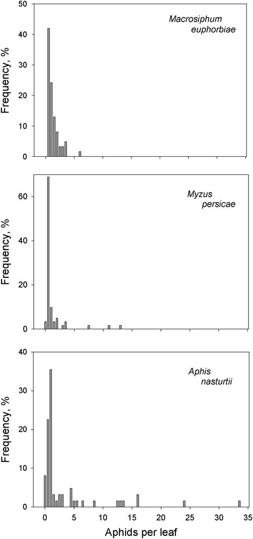
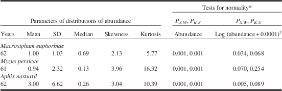
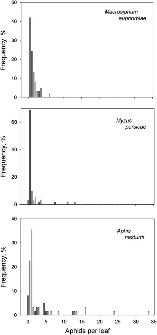
Mean annual densities of M. euphorbiae and M. persicae were near one aphid per leaf, whereas that of A. nasturtii was three aphids per leaf (Table 1). Annual abundance was not normally distributed for any of the species, with the median lower than the mean (Table 1), and distributions strongly skewed with a small proportion of years having high abundance (Fig. 1). The high abundance tail of the distribution was particularly long for A. nasturtii. No M. persicae or A. nasturtii were present in three and eight of the 62 years, respectively, but in some years their abundance reached 13 and 33 aphids per leaf, respectively, more than twice the peak abundance of six aphids per leaf for M. euphorbiae, which was always present. The abundance of M. persicae approximated a lognormal distribution based on the Shapiro–Wilk Test and all three species passed the Kolmogorov–Smirnov Test when log-transformed (SYSTAT Software 2009) (Table 1).
The distributions of annual abundance (aphids per leaf) for three species of aphid sampled in potato plots for 62 years. If no grey bar is present, no year had that aphid abundance.
Annual abundance of aphids (aphids per leaf) on potatoes sampled for 61 or 62 years.
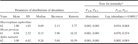
Notes:
* P S-W (fails Shapiro–Wilk test if P<0.05), P K-S (fails Kolmogorov–Smirnov test if P<0.05).
† 0.0001 was added to abundance to eliminate 0-values.
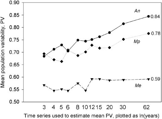
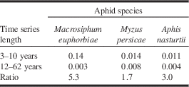
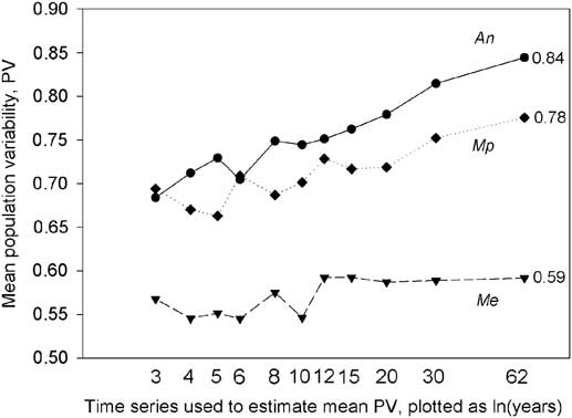
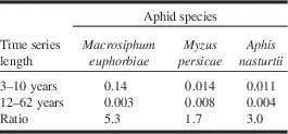
For M. euphorbiae, PV62 was 0.59, for M. persicae, 0.78, and for A. nasturtii, 0.84 (Fig. 2). Note that PV62 for A. nasturtii was 0.01 higher than PV58 reported by Lamb et al. (Reference Lamb, MacKay and Alyokhin2011). Mean PV, estimated for time series of 3–62 years, deviated from the trend for the relationship of mean PV and time series length, particularly for time series up to about 12 years, but was more uniform for longer time series (Fig. 2). The mean deviations (calculated as the residual variability not explained by linear regression, SYSTAT Software 2009) were 1.7 to 5.3 times higher for short (3–10 years) than for long (12–62 years) time series (Table 2). For all three species, but particularly M. euphorbiae, mean PV was more uniform for time series of 12–15 years or longer than for shorter ones (Fig. 2; Table 2).
Mean population variability (PV, Heath Reference Heath2006) for three species of aphid, Macrosiphum euphorbiae (Me), Myzus persicae (Mp), and Aphis nasturtii (An) in potato plots, estimated for time series of 3–62 years for each species. The sample size for each mean ranges from 20 for a three-year time series to one for a 62-year time series (n=60/time series length). Estimates of mean PV62 are provided.
Mean deviation of population variability (PV, see text) for a regression of mean PV on time series length (see Fig. 2) for short (3–10 years, n=6) or long time series (12–62 years, n=5), and the ratio of mean deviations for the short and long time series.
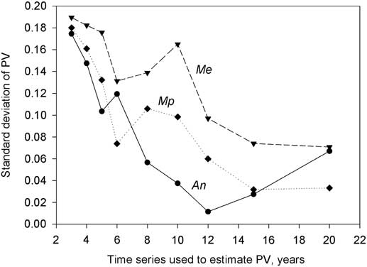
Estimates of PV based on nine time series from 3–20 years (n=20–3), 27 time series for the three aphid species, were normally distributed based on the Shapiro–Wilk Test (SYSTAT Software 2009), except the four-year time series for A. nasturtii. The fact that PV was usually normally distributed justified using standard deviation to quantify the variability of this parameter. The standard deviation of PV declined with increasing length of the time series reaching a low at 12 or 15 years (Fig. 3).
Standard deviation of population variability (PV, Heath Reference Heath2006) for three species of aphid, Macrosiphum euphorbiae (Me), Myzus persicae (Mp), and Aphis nasturtii (An) in potato plots, estimated for time series of 3–20 years from a 60-year time series of annual abundance for each species (n=60/time series length).
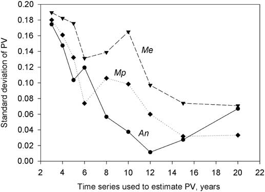
Standard deviation was highest for M. euphorbiae (Fig. 3), although this species had the lowest mean PV at all time series (Fig. 2). Based on a paired t-test (SYSTAT Software 2009) for the nine time series from 3–20 years, the standard deviations for M. euphorbiae differed from those for M. persicae and A. nasturtii (df=8, P<0.003), but the latter two species did not differ (df=8, P=0.355). For the 15-year time series, coefficients of variation (standard deviation as a % of the mean) ranged from 3.5 for M. persicae and 4.5 for A. nasturtii to 12.5 for M. euphorbiae.
A two-sample t-test assuming separate variances (SYSTAT Software 2009) showed that PV was lower for M. euphorbiae than for M. persicae or A. nasturtii for each of the nine time series from 3 to 20 years (P⩽0.05). However, M. persicae (PV61 =0.78) was detected as having a lower PV than A. nasturtii (PV62=0.84) only for a 15-year time series (P=0.037, P>0.05 for other time series).
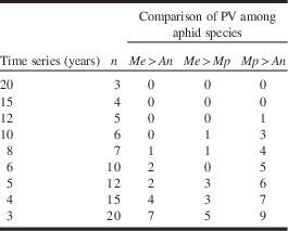
Macrosiphum euphorbiae had a PV62=0.59, 19–25 units lower than the other two species (Fig. 2). Assuming the longest time series, 62 years, provided the best estimate of PV, this species was expected to have a lower PV than the other species regardless of time series length (Fig. 2). That result was observed for time series of 12–20 years, but not always for time series of 3–10 years (Table 3). Myzus persicae (PV61=0.78) was expected to have a lower PV than A. nasturtii (PV62=0.84), but this difference was only consistently evident at intervals of 15 or 20 years (Table 3). For M. persicae with a PV62 0.06 lower than A. nasturtii, the estimate of PV at time series of 3–10 years was lower than for A. nasturtii only about 50% of the time (Table 3). In other words, when PV62 differed between species by 0.25, a single time series would not always correctly differentiate PV for the two species unless the time series was at least 12 years long. If the difference between PV62 for two species was small, for example, 0.06, then a time series of 15 years was required to reliably discriminate two species (Table 3).
The number of cases where the observed population variability (PV, see text) of Macrosiphum euphorbiae (Me, PV=0.59 over 62 years) exceeds that of Myzus persicae (Mp, PV=0.78 over 61 years) or Aphis nasturtii (An, PV=0.84 over 62 years), and the PV of Mp exceeds that of An, for time series of 3–20 years from a 60-year time series.
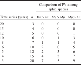
Note: Estimates of PV were compared for pairs of the three species and each time series, giving, for example, 20 comparisons for each pair for a three-year times series.
Discussion
The frequency distributions of annual abundance for the three aphids were characterised by a preponderance of low abundances with some high abundance years, the frequency and level of high abundance increased from M. euphorbiae (PV62=0.59), to M. persicae (PV61=0.78), and A. nasturtii (PV62=0.84). These three patterns cover a sufficiently broad range, at least for PV>0.5, that they can be expected to be representative of organisms that have many years of low abundance with occasional outbreaks.
For the three species, estimates of mean PV were less uniform for time series of 10–12 years or less, than for longer ones. Therefore, a single short time series was less likely to provide an accurate estimate of PV than a long one. Consistent with this conclusion is the observation that standard deviation of PV declined as the time series used to calculate PV increased, at least for short time series. The standard deviations of PV reached a minimum at time series of 12–15 years and did not decline further at 20 years. A decline in the standard deviation of PV with increasing time interval was expected based on results for three theoretical distributions (Heath Reference Heath2006). The similarity in standard deviations between 15-year and 20-year time series for these three aphids occurred at shorter time series than expected for normal or Cauchy distributions of abundance, but was consistent with that for a log-normal distribution (fig. 5 in Heath Reference Heath2006). The frequency distributions of annual abundance for the three aphids were not distinguishable from log-normal by Kolmogorov–Smirnov tests.
The standard deviation of PV for M. euphorbiae was consistently higher than those for the other two species, regardless of time series length. PV15 for M. euphorbiae exhibited a higher level of variability over time relative to its mean (coefficient of variation=12.5) than that of the other two species (coefficients of variation=3.5 and 4.5). The life history traits of M. euphorbiae that cause PV to be less uniform over time than PV for the other two species remain to be determined. This result is the first quantitative demonstration that different species can exhibit different variances in PV as well as different levels of PV. Although estimates of PV were usually normally distributed, justifying parametric tests for comparison among species or populations, differences in variance among estimates of PV would limit which parametric tests are appropriate.
The three species of aphids had different levels of PV (Lamb et al. Reference Lamb, MacKay and Alyokhin2011, Reference Lamb, MacKay and Alyokhin2013), confirmed here by the consistent differences between estimates when time series were 15–62 years long. For PV62, M. euphorbiae differs by 0.19 and 0.25 units of PV on a 0–1 scale from M. persicae and A. nasturtii, respectively. The latter two species differed from each other by only 0.06. Not surprisingly, the reliability with which the estimates of PV for the species could be differentiated depended on how many units of PV separated them. M. euphorbiae was always (given a sample of five to six time series) differentiated from M. persicae and A. nasturtii by time series intervals of 10 and 12 years or more, respectively. However, the PV of M. persicae and A. nasturtii were consistently separated using a time series of 15 years or longer.
Based on these three aphid species, we conclude that a time series length of 15 years should be adequate for estimating PV for most populations, when the objective is to make reliable interspecific comparisons of PV. This conclusion does not necessarily mean that studies based on shorter time series cannot be used for inter-specific comparisons. For example, Cappuccino (Reference Cappuccino1987) compared the population variability of two aphids sampled from the same plant population over four years. She concluded, based on standard deviation of the log of annual abundance, that one species was more variable in abundance than the other. The PV for these two aphid populations were 0.98 and 0.39 (calculated from fig. 2, Cappuccino Reference Cappuccino1987). With such a large difference in PV between species, there is little doubt that for the period of the study, one species had a less variable population than the other, even with a time series of four years. In a seven-year study, Dalin et al. (Reference Dalin, Kindvall and Björkman2009) found that a leaf beetle in plantations of willow had a PV of 0.60 compared with 0.42 in natural willow stands. The conclusion that these populations were less variable in natural stands than in monocultures was justified because 20 pairs of populations were considered. Nevertheless, Dalin et al. (Reference Dalin, Kindvall and Björkman2009) found substantial overlap in PV between monocultures (PV range=0.24–0.80) and natural stands (PV range=0.20–0.64). Any single estimate of PV for this leaf beetle based on a time series of only seven years would have low precision for estimating the PV for a population or the species.
For three potato-infesting aphids, the answer to the question, “How many years are required?”, is 15 years. A 15-year time series minimises the standard deviation of the estimate, and makes it possible to discriminate PV values that differ by as little as 0.06 on a 0–1 scale. The frequency distributions of annual abundance for these species show a range of patterns from highly clumped at low densities, but persistent (M. euphorbiae), to less persistent with occasional high density years (A. nasturtii). Therefore, this recommendation should apply to many species.