Introduction
As finite and non-renewable natural resources, spectrum resources are becoming increasingly scarce with the rapid development of communication technologies. Consequently, modern communication systems are required to operate within an increasingly crowded spectrum environment [Reference Zheleva, Anderson, Aksoy, Johnson, Affinnih and DePree1]. Furthermore, microwave components in these systems operate under increasingly complex electromagnetic conditions, which may induce various interference issues such as crosstalk, intermodulation, and harmonic distortions, thereby affecting the normal operation of communication equipment.
Nonreciprocal devices exhibit unidirectional signal transmission characteristics, enabling the isolation of in-band backward interference signals and thereby improving circuit interference immunity and spectrum utilization [Reference Kord, Sounas and Alù2]. These devices have been used in various systems, including wireless communication systems, radar systems, and biomedical systems [Reference Nagulu and Krishnaswamy3]. Conventional nonreciprocal devices based on ferrite materials suffer from inherent limitations including bulky size, high cost, and poor integrability with other circuits [Reference Fay and Comstock4–Reference Kord, Sounas and Alù7], which has motivated extensive research on magnetic-free nonreciprocal implementations. Recent studies have demonstrated that spatio-temporal modulation (STM) is an effective approach for achieving magnetic-free nonreciprocal characteristics. In [Reference Fleury, Sounas, Sieck, Haberman and Alù8], angular-momentum biasing implemented through STM breaks time-reversal symmetry, thereby enabling the realization of a magnetless acoustic circulator. Similarly, in the electronic domain, nonreciprocal characteristics have been demonstrated through continuous permittivity modulation of a ring resonator [Reference Sounas, Caloz and Alù9]. Subsequently, implementations of magnetless circulators were demonstrated using STM of lumped LC resonators in both Δ- and Y-topology configurations [Reference Estep, Sounas, Soric and Alù10, Reference Estep, Sounas and Alù11]. Further extensions of this concept have since been reported in [Reference Kord, Sounas and Alù12–Reference Yu, Michetti, Kord, Sounas, Pop, Kulik, Pirro, Qian, Alù and Rinaldi16]. Later [Reference Wu and Liu17–Reference Wu and Liu20], report on related work concerning isolators and circulators based on time-modulated resonators.
A novel STM nonreciprocal bandpass filter (BPF) was proposed in [Reference Wu, Liu, Hickle, Peroulis, Gómez-Díaz and Melcón21], employing the time-modulated resonators (TMRs) realized by modulating reverse-bias varactor diodes in a lumped LC resonator with progressively phase-shifted sinusoidal signals. Here, the nonreciprocal behavior of the circuit arises from the nonlinear capacitance property of a varactor diode under reverse bias, which produces intermodulation (IM) products when modulated within the resonators. A difference in RF power distribution between forward and reverse paths among these IM products leads to nonreciprocal circuit performance. Subsequent studies have further extended this approach, including implementations based on lumped elements [Reference Simpson and Psychogiou22, Reference Simpson and Psychogiou23] where [Reference Simpson and Psychogiou22] achieved tunable center frequency and [Reference Simpson and Psychogiou23] proposed a fully reconfigurable design. Additionally [Reference Alvarez-Melcon, Wu, Zang, Liu and Gomez-Diaz24], analyzed nonreciprocal BPFs using time-varying coupling matrix formalism, while [Reference Dutta, Kumar and Ram25] and [Reference Dutta, Kumar and Ram26] introduced a 3D coupling matrix concept and a PSO-based optimization algorithm for parameter configuration, respectively. In [Reference Chaudhary and Jeong27], a nonreciprocal BPF integrated with an impedance-matching circuit was proposed. In [Reference Wu, Nafe, Melcón, Gómez-Díaz and Liu28–Reference Wu, Nafe, Melcón, Gómez-Díaz and Liu30], microstrip nonreciprocal BPFs were implemented using half- and quarter-wavelength TMRs. Subsequent works [Reference Chatzichristodoulou, Arain, Pavlou, Vassiliou, Psychogiou, Nikolaou and Vryonides31, Reference Chaudhary and Jeong32] achieved quasi-elliptic responses to improve selectivity. By coupling the static resonator with TMRs, an enhanced reverse isolation bandwidth is achieved in [Reference Chaudhary and Jeong33] without the need for additional TMRs. Finally [Reference Chaudhary and Jeong34] demonstrated an ultrawide high reverse isolation bandwidth design using a four-stage cascaded TMR configuration. Although extensive research has been conducted on nonreciprocal bandpass filters, previous works have primarily focused on in-band forward transmission characteristics, reverse isolation, reconfigurability, and impedance matching to enhance circuit applicability. Notably, no prior investigation has been reported on stopband reflected wave absorption. Although the nonreciprocal characteristics effectively isolate in-band reverse interference signals, the stopband reflected waves can still have adverse effects on adjacent circuits.
With the rapid advancement of wireless communication technologies, balanced microwave circuits have become increasingly preferred over their single-ended counterparts. Compared to single-ended circuits, balanced architectures can suppress common-mode (CM) noise, provide better immunity to external interference and electromagnetic crosstalk, and enhance signal integrity and overall system performance [Reference Martin and Medina35]. Notably, balanced microwave circuits with CM and differential-mode (DM) reflectionless characteristics can effectively absorb unwanted CM noise and DM signals [Reference Zhang, Wu, Wang and Yan36–Reference Zhao, Wei, Yang and Gómez-García38]. This property can further solve potential issues, such as amplifier instability and mixer intermodulation interference, caused by reflected waves of the reflection-based CM noise suppression and reflection-based DM stopband attenuation.
A balanced nonreciprocal BPF based on time-modulated resonators was first proposed in [Reference Simpson, Vryonides, Nikolaou and Psychogiou39]. However, this design suffers from drawbacks such as a bulky and complex structure, as well as a narrow reverse isolation bandwidth (BW). Compared with the design in [Reference Simpson, Vryonides, Nikolaou and Psychogiou39], the work in [Reference Han, Wang, Liu, Gao and Fang40] utilizes stepped impedance resonators and TMRs to implement a compact balanced nonreciprocal BPF featuring simplified feeding and enhanced reverse isolation BW. The work in [Reference Han, Wang, Liu, Gao and Fang41] further simplifies the circuit design by co-designing feed circuits and CM suppression circuits, thereby reducing complexity. Furthermore, while CM noise is suppressed through reflection, the radiated emissions generated by CM noise are significantly stronger than those of the differential signals, potentially degrading system reliability. To address this issue, a balanced nonreciprocal filter with CM reflectionless characteristics is introduced in [Reference Han, Wang, Liu and Fang42], which effectively absorbs unwanted CM noise. Nevertheless, the design proposed in [Reference Han, Wang, Liu and Fang42] remains ineffective in solving the negative effects of reflected waves of the reflection-based DM stopband attenuation.
To further solve the negative effects of reflected waves of the reflection-based DM stopband attenuation, this paper proposes a balanced nonreciprocal BPF with both CM and DM reflectionless characteristics. The proposed circuit integrates DM and CM noise absorption structure, differential filter, and isolator. Conventional TMR-based nonreciprocal implementations suffer from degraded reflection zeros. This issue is addressed through the introduction of a CM and DM reflectionless structure, which effectively absorbs stopband signals in DM. The circuit features a symmetrical design about the central horizontal plane. By exploiting the different boundary conditions of the horizontal symmetry plane under CM and DM excitations, effective CM suppression is achieved, and the feeding circuit is arranged reasonably. The CM and DM reflectionless characteristics are achieved simultaneously by symmetrically loading coupled lines terminated with absorption resistors at the input/output ports. This configuration enables simultaneous absorption of both DM and CM reflected signals by utilizing the different boundary conditions of DM and CM under their respective excitations. The circuit design methodology is analytically described through matrix-based calculations and parametric studies. Furthermore, a 1.5-GHz microstrip prototype is fabricated and experimentally characterized to validate the theory and methodology of the proposed CM and DM reflectionless balanced nonreciprocal BPF.
Theoretical analysis and design
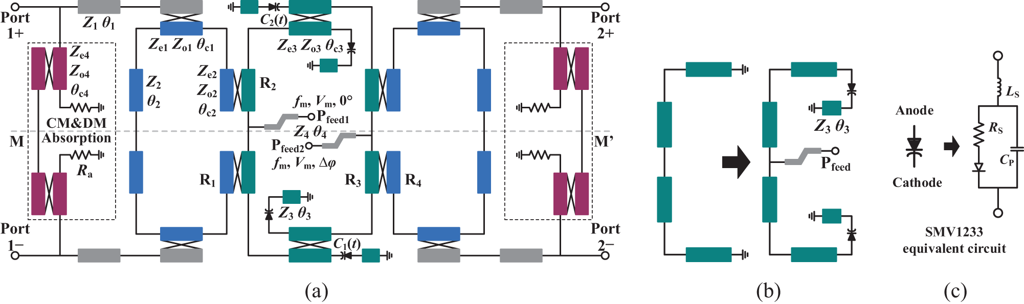
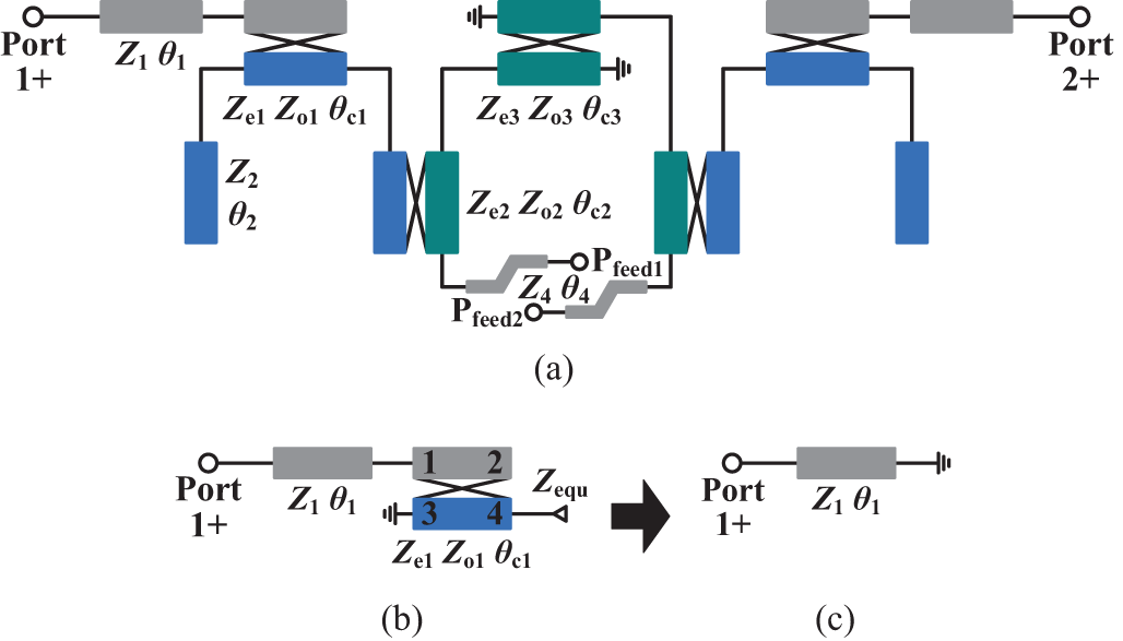
Figure 1(a) shows the circuit diagram of the proposed CM and DM reflectionless balanced nonreciprocal BPF. The structure comprises two pairs of balanced ports (1 ±, 2±) and two modulation ports (Pfeed1, Pfeed2). Based on the S-parameters of the four-port single-ended network, the mixed-mode S-parameters for CM and DM responses can be derived as follows:
 \begin{equation}\left\{ {\begin{array}{*{20}{l}}
{{S_{{\text{cc11}}}} = {{\left( {{S_{{\text{1}} + {\text{1}} + }} + {S_{{\text{1}} + {\text{1}} - }} + {S_{{\text{1}} - {\text{1}} + }} + {S_{{\text{1}} - {\text{1}} - }}} \right)} \mathord{\left/
{\vphantom {{\left( {{S_{{\text{1}} + {\text{1}} + }} + {S_{{\text{1}} + {\text{1}} - }} + {S_{{\text{1}} - {\text{1}} + }} + {S_{{\text{1}} - {\text{1}} - }}} \right)} 2}} \right.
} 2}} \\
{{S_{{\text{cc12}}}} = {{\left( {{S_{{\text{1}} + {\text{2}} + }} + {S_{{\text{1}} + {\text{2}} - }} + {S_{{\text{1}} - 2 + }} + {S_{{\text{1}} - {\text{2}} - }}} \right)} \mathord{\left/
{\vphantom {{\left( {{S_{{\text{1}} + {\text{2}} + }} + {S_{{\text{1}} + {\text{2}} - }} + {S_{{\text{1}} - 2 + }} + {S_{{\text{1}} - {\text{2}} - }}} \right)} 2}} \right.
} 2}} \\
{{S_{{\text{cc21}}}} = {{\left( {{S_{{\text{2}} + {\text{1}} + }} + {S_{{\text{2}} + {\text{1}} - }} + {S_{{\text{2}} - {\text{1}} + }} + {S_{{\text{2}} - {\text{1}} - }}} \right)} \mathord{\left/
{\vphantom {{\left( {{S_{{\text{2}} + {\text{1}} + }} + {S_{{\text{2}} + {\text{1}} - }} + {S_{{\text{2}} - {\text{1}} + }} + {S_{{\text{2}} - {\text{1}} - }}} \right)} 2}} \right.
} 2}} \\
{{S_{{\text{cc22}}}} = {{\left( {{S_{{\text{2}} + {\text{2}} + }} + {S_{{\text{2}} + {\text{2}} - }} + {S_{{\text{2}} - {\text{2}} + }} + {S_{{\text{2}} - {\text{2}} - }}} \right)} \mathord{\left/
{\vphantom {{\left( {{S_{{\text{2}} + {\text{2}} + }} + {S_{{\text{2}} + {\text{2}} - }} + {S_{{\text{2}} - {\text{2}} + }} + {S_{{\text{2}} - {\text{2}} - }}} \right)} 2}} \right.
} 2}}
\end{array}} \right.\end{equation}
 \begin{equation}\left\{ {\begin{array}{*{20}{l}}
{{S_{{\text{dd11}}}} = {{\left( {{S_{{\text{1}} + {\text{1}} + }} - {S_{{\text{1}} + {\text{1}} - }} - {S_{{\text{1}} - {\text{1}} + }} + {S_{{\text{1}} - {\text{1}} - }}} \right)} \mathord{\left/
{\vphantom {{\left( {{S_{{\text{1}} + {\text{1}} + }} - {S_{{\text{1}} + {\text{1}} - }} - {S_{{\text{1}} - {\text{1}} + }} + {S_{{\text{1}} - {\text{1}} - }}} \right)} 2}} \right.
} 2}} \\
{{S_{{\text{dd12}}}} = {{\left( {{S_{{\text{1}} + {\text{2}} + }} - {S_{{\text{1}} + {\text{2}} - }} - {S_{{\text{1}} - 2 + }} + {S_{{\text{1}} - {\text{2}} - }}} \right)} \mathord{\left/
{\vphantom {{\left( {{S_{{\text{1}} + {\text{2}} + }} - {S_{{\text{1}} + {\text{2}} - }} - {S_{{\text{1}} - 2 + }} + {S_{{\text{1}} - {\text{2}} - }}} \right)} 2}} \right.
} 2}} \\
{{S_{{\text{dd21}}}} = {{\left( {{S_{{\text{2}} + {\text{1}} + }} - {S_{{\text{2}} + {\text{1}} - }} - {S_{{\text{2}} - {\text{1}} + }} + {S_{{\text{2}} - {\text{1}} - }}} \right)} \mathord{\left/
{\vphantom {{\left( {{S_{{\text{2}} + {\text{1}} + }} - {S_{{\text{2}} + {\text{1}} - }} - {S_{{\text{2}} - {\text{1}} + }} + {S_{{\text{2}} - {\text{1}} - }}} \right)} 2}} \right.
} 2}} \\
{{S_{{\text{dd22}}}} = {{\left( {{S_{{\text{2}} + {\text{2}} + }} - {S_{{\text{2}} + {\text{2}} - }} - {S_{{\text{2}} - {\text{2}} + }} + {S_{{\text{2}} - {\text{2}} - }}} \right)} \mathord{\left/
{\vphantom {{\left( {{S_{{\text{2}} + {\text{2}} + }} - {S_{{\text{2}} + {\text{2}} - }} - {S_{{\text{2}} - {\text{2}} + }} + {S_{{\text{2}} - {\text{2}} - }}} \right)} 2}} \right.
} 2}}
\end{array}} \right.\end{equation}
where the subscript d represents the DM, and the subscript c represents the CM.
(a) Circuit diagram of the proposed CM and DM reflectionless balanced nonreciprocal BPF. (b) Evolution of time-modulated resonator. (c) The equivalent circuit of varactor diodes.

The microstrip circuit is divided into two blocks: a balanced nonreciprocal BPF structure and a CM and DM reflectionless structure. The balanced nonreciprocal BPF structure comprises two symmetric static resonators Ri (i = 1, 4; θ 2 = θ c1 = θ c2 = π/2), indicated by blue fill; two symmetric time-modulated resonators Ri (i = 2, 3; θ 3, θ c2 = θ c3 = π/2) that load varactor diodes, indicated by dark cyan fill; and microstrip transmission lines (θ 1 = θ c1 = π/2) and feed lines (θ 4 = π/2), indicated by gray fill. The CM and DM reflectionless structure, symmetrically arranged about the horizontal symmetry plane (MM’), comprises two pairs of resistively terminated parallel-coupled lines (θ c4 = π/2, R a). Figure 1(b) shows that the TMR is derived from a λ-short-circuited resonator. Utilizing the λ-short-circuited resonator, a balanced BPF can be realized. To compensate for the resonant frequency shift caused by the loaded varactor diode, a compensation microstrip line (θ 3) is incorporated. The electrical length θ 3 of the compensation microstrip line and the nominal DC-bias capacitance C 0 of the varactor diode satisfy Equation (3).
 \begin{equation}{Z_3}\tan {\theta _3} - 1/\left( {\omega {\kern 1pt} {C_0}} \right) = 0\end{equation}
where ω represents the angular frequency. In DM excitation, the center of the λ-short-circuited resonator acts as a virtual ground point. By integrating a λ/4 microstrip feed line at this node, inherent isolation between the balanced ports and the modulation ports can be intrinsically maintained. The design employs Skyworks SMV1233 varactor diodes, which equivalent circuit is shown in Figure 1(c). The parasitic parameters of the Skyworks SMV1233 varactor diodes can be extracted directly from the manufacturer’s datasheet [43]. The circuit’s working principle is described below, beginning with the balanced BPF structure incorporating a λ-short-circuited resonator.
Balanced DM bandpass filter structure
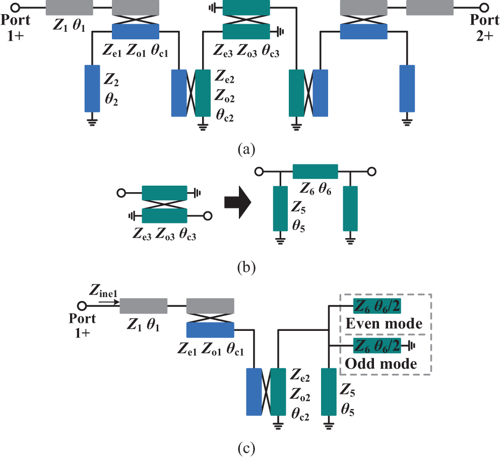
Figure 2(a) illustrates the balanced BPF DM equivalent circuit. According to microwave circuit theory [Reference Cameron, Kudsia and Mansour44], a λ/4 short-circuited transmission line (θ 2) is equivalent to an open-circuited at its junction with the coupled line (θ c1). Furthermore, Figure 2(b) depicts the λ/4 short-circuited parallel coupled line (θ c3) along with its equivalent circuit (θ 5 = θ 6 = π/2). By equating the ABCD-matrix of the short-circuited parallel coupled line and its equivalent circuit, the following relationships are derived.
 \begin{equation}\left\{ {\begin{array}{*{20}{l}}
{{Z_5} = {Z_{{\text{e}}3}}} \\
{{Z_6} = \frac{{2{Z_{{\text{e}}3}}{Z_{{\text{o}}3}}}}{{{Z_{{\text{e}}3}} - {Z_{{\text{o}}3}}}}}
\end{array}} \right.\end{equation}
Consequently, the even- and odd-mode equivalent circuits of the balanced BPF’s DM equivalent circuit can be derived, as shown in Figure 2(c). Based on the cascaded transmission line and coupled line relationship shown in Figure 2(c), the even- and odd-mode input impedances (Z ine1, Z ino1) are derived as follows:
 \begin{equation}{Z_{{\text{ine1}}}} = \frac{{{Z_6}{X_1}\cos \left( {\frac{\theta }{2}} \right) - {\text{j}}{X_6}\sin \left( {\frac{\theta }{2}} \right)}}{{{Z_6}{X_2}\cos \left( {\frac{\theta }{2}} \right) - {\text{j}}{X_5}\sin \left( {\frac{\theta }{2}} \right)}}\end{equation}
 \begin{equation}{Z_{{\text{ino1}}}} = \frac{{{Z_6}{X_1}\sin \left( {\frac{\theta }{2}} \right) + {\text{j}}{X_6}{\text{cos}}\left( {\frac{\theta }{2}} \right)}}{{{Z_6}{X_2}\sin \left( {\frac{\theta }{2}} \right) + {\text{j}}{X_5}{\text{cos}}\left( {\frac{\theta }{2}} \right)}}\end{equation}
where
 \begin{equation}X_1=\frac{\text{j}X_6}{Z_5\tan\theta}+\frac{\text{j2}X_9\cot\theta}{Z_\text{e2}-Z_{\text{o}2}}-\frac{X_3X_{10}}{X_4}\end{equation}
 \begin{equation}X_2=\frac{\text{j}X_5}{Z_5\tan\theta}+\frac{\text{j2}X_7\cot\theta}{Z_\text{e2}-Z_{\text{o}2}}-\frac{X_3X_8}{X_4}\end{equation}
 \begin{equation}{X_3} = {\left( {{Z_{{\text{e}}2}} + {Z_{{\text{o}}2}}} \right)^2} - 4{Z_{{\text{e}}2}}{Z_{{\text{o}}2}}/{\sin ^2}\theta \end{equation}
 \begin{equation}X_4=\left(Z_{\text{e}2}+Z_{\text{o}2}\right)\left(Z_{\text{e}2}-Z_{\text{o}2}\right)\end{equation}
 \begin{equation}{X_5} = \frac{{\left( {{Z_{{\text{e}}2}} + {Z_{{\text{o}}2}}} \right){X_7}}}{{{Z_{{\text{e}}2}} - {Z_{{\text{o}}2}}}} - \frac{{{\text{j2}}{X_8}{Z_{{\text{e}}2}}{Z_{{\text{o}}2}}\cot \theta }}{{{Z_{{\text{e}}2}} - {Z_{{\text{o}}2}}}}\end{equation}
 \begin{equation}{X_6} = \frac{{\left( {{Z_{{\text{e}}2}} + {Z_{{\text{o}}2}}} \right){X_9}}}{{{Z_{{\text{e}}2}} - {Z_{{\text{o}}2}}}} - \frac{{{\text{j2}}{X_{10}}{Z_{{\text{e}}2}}{Z_{{\text{o}}2}}\cot \theta }}{{{Z_{{\text{e}}2}} - {Z_{{\text{o}}2}}}}\end{equation}
 \begin{equation}{X_7} = {X_{12}} + \frac{{{\text{j}}{X_{11}}{{\sin }^2}\theta }}{{2{Z_1}\left( {{Z_{{\text{e}}1}} - {Z_{{\text{o}}1}}} \right)}}\end{equation}
 \begin{equation}{X_8} = \frac{{{\text{j}}2\sin \theta \cos \theta }}{{{Z_{{\text{e}}1}} - {Z_{{\text{o}}1}}}} + \frac{{{\text{j}}\left( {{Z_{{\text{e}}1}} + {Z_{{\text{o}}1}}} \right)\sin \theta \cos \theta }}{{{Z_1}\left( {{Z_{{\text{e}}1}} - {Z_{{\text{o}}1}}} \right)}}\end{equation}
 \begin{equation}{X_9} = \frac{{{X_{11}}\sin \theta \cos \theta }}{{2\left( {{Z_{{\text{e}}1}} - {Z_{{\text{o}}1}}} \right)}} + \frac{{{\text{j}}{{\text{Z}}_{\text{1}}}\left( {{Z_{{\text{e}}1}} + {Z_{{\text{o}}1}}} \right)\sin \theta \cos \theta }}{{{Z_{{\text{e}}1}} - {Z_{{\text{o}}1}}}}\end{equation}
 \begin{equation}{X_{10}} = {X_{12}} - \frac{{2{Z_1}{{\sin }^2}\theta }}{{{Z_{{\text{e}}1}} - {Z_{{\text{o}}1}}}}\end{equation}
 \begin{equation}{X_{11}} = {\text{j}}{\left( {{Z_{{\text{e}}1}} + {Z_{{\text{o}}1}}} \right)^2} - \frac{{{\text{j4}}{Z_{{\text{e}}1}}{Z_{{\text{o}}1}}}}{{{{\sin }^2}\theta }}\end{equation}
 \begin{equation}{X_{12}} = \frac{{\left( {{Z_{{\text{e}}1}} + {Z_{{\text{o}}1}}} \right){{\cos }^2}\theta }}{{{Z_{{\text{e}}1}} - {Z_{{\text{o}}1}}}}\end{equation}
and θ = π/2 at the center frequency f 0 = 1.5 GHz.
Then, the S-parameters (S dd11 and S dd21) of the balanced BPF under DM excitation can be derived as Equations (19) and (20).
 \begin{equation}{S_{{\text{dd}}11}}\; = \;\frac{{{\Gamma _{{\text{e1}}}} + {\Gamma _{{\text{o1}}}}}}{2} = \frac{{{Z_{{\text{ine1}}}}{Z_{{\text{ino1}}}} - Z_0^2}}{{\left( {{Z_{{\text{ine1}}}} + {Z_0}} \right)\,\left( {{Z_{{\text{ino1}}}} + {Z_0}} \right)}}\end{equation}
 \begin{equation}{S_{{\text{dd21}}}} = \frac{{{\Gamma _{{\text{e1}}}} - {\Gamma _{{\text{o1}}}}}}{2} = \frac{{{Z_0}{Z_{{\text{ine1}}}} - {Z_0}{Z_{{\text{ino1}}}}}}{{\left( {{Z_{{\text{ine1}}}} + {Z_0}} \right)\,\left( {{Z_{{\text{ino1}}}} + {Z_0}} \right)}}\end{equation}
where
 \begin{equation}\Gamma_{\text{e}1}=\frac{Z_{\text{ine}1}-Z_0}{Z_{\text{ine}1}+Z_0},\;\;\;\;\;\;\;\,\Gamma_{\text{o}1}=\frac{Z_{\text{ino}1}-Z_0}{Z_{\text{ino}1}+Z_0}\end{equation}
Here, Z 0 denotes the port impedance, while Γ e1 and Γ o1 represent the reflection coefficients of the even- and odd-mode equivalent circuits, respectively, as shown in Figure 2(c). Table 1 shows a set of reference values with a ripple factor L P = 0.043 dB, corresponding to a fractional BW of 8.4%.
(a) DM equivalent circuit of the balanced BPF. (b) Equivalent circuit of the short-circuited parallel coupled lines. (c) Derived even-mode and odd-mode equivalent circuits corresponding to Figure 2(a).

Balanced DM BPF reference values (unit Ω)

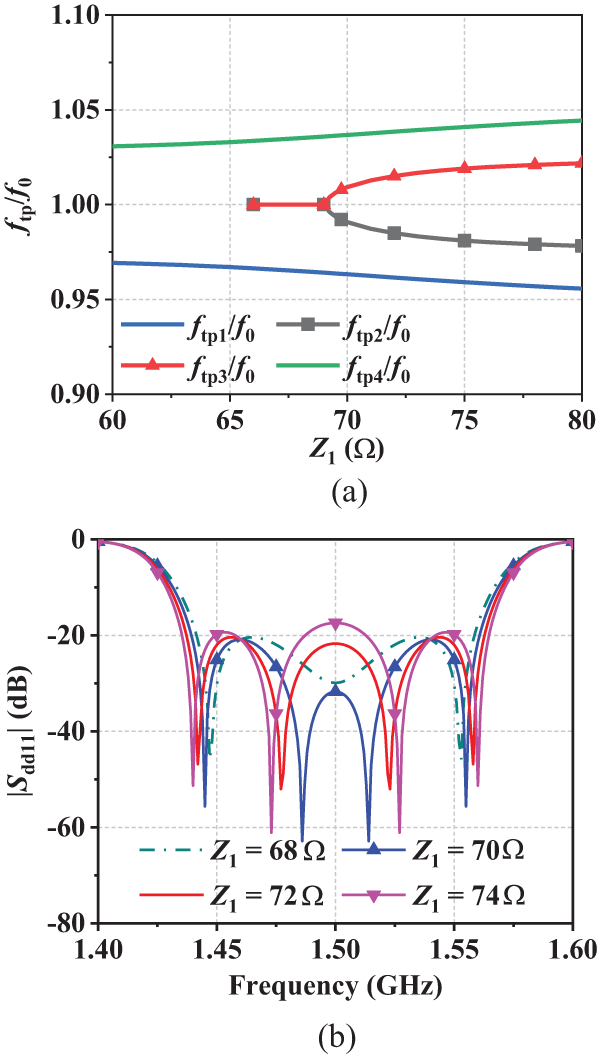
Equation (19) indicates that the DM transmission poles (TPs) depend on the characteristic impedance of the transmission line (θ 1) as well as the even- and odd-mode characteristic impedances of the coupled lines (θ c1, θ c2, θ c3). Using the parameters specified in Table 1, a comprehensive parametric analysis is conducted for both the transmission line and the coupled lines. Figure 3(a) shows the calculated TPs (f tp1, f tp2, f tp3, f tp4) as a function of the characteristic impedance Z 1, demonstrating the variation in both the number of TPs and their normalized positional relationships. For clarity, Figure 3(b) shows the corresponding S-parameters curves (|S dd11|) of the balanced BPF, computed using Equation (19). The results indicate that variations in characteristic impedance Z 1 primarily influence the relative positions between f tp2 and f tp3, thereby governing the impedance matching characteristics near the center frequency of the passband.
Calculated (a) TPs and (b) |S dd11| versus different Z 1.

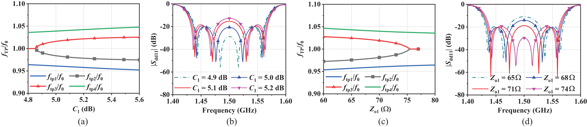
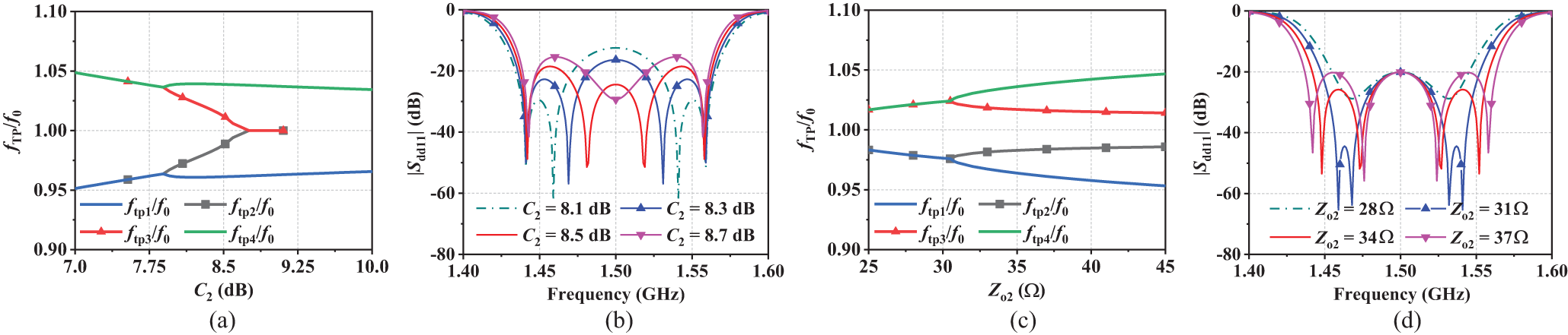
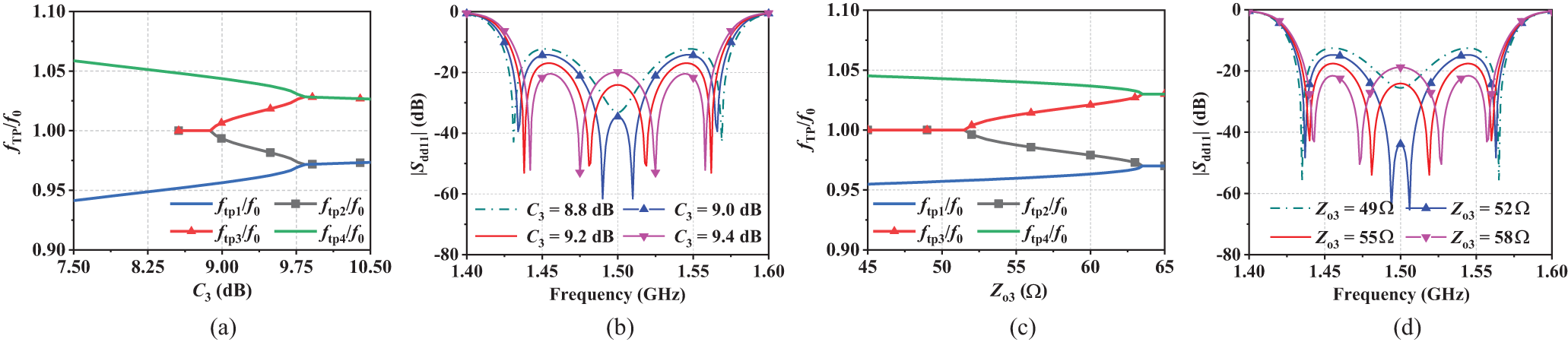
The calculated TPs versus coupling coefficient C 1 are illustrated in Figure 4(a), where the odd-mode characteristic impedance Z o1 is fixed at 71.6 Ω. When the coupling coefficient C 1 exceeds 4.86 dB, four TPs emerge. As C 1 further increases, the relative positions of f tp1 and f tp2, as well as f tp3 and f tp4, remain unchanged. However, the spacing between f tp2 and f tp3 widens. As shown in Figure 4(b), this increased spacing results in a higher peak in the middle of the |S dd11| curve, deteriorating impedance matching in the corresponding frequency band. Furthermore, Figure 4(c) illustrates the variation of the TPs with respect to Z o1, while the coupling C 1 is fixed at 5.0 dB. The corresponding |S dd11| responses are plotted in Figure 4(d). When Z o1 is below 75 Ω, four TPs are observed in Figure 4(c). The relative positions of f tp1 and f tp2, as well as f tp3 and f tp4, remain nearly constant. However, as the spacing between the f tp2 and f tp3 decreases, the peak in the middle of the |S dd11| curve is reduced, leading to improved impedance matching over the corresponding frequency band. Similarly, the influence of the coupled lines (θ c2, θ c3) on the TPs can be analyzed, with their corresponding |S dd11| responses plotted in Figures 5 and 6. In Figure 5(a,b), the odd-mode characteristic impedance Z o2 is fixed at 37.1 Ω, while in Figure 5(c,d), the coupling coefficient C 2 is fixed at 8.4 dB. Likewise, Figure 6(a,b) feature a fixed odd-mode characteristic impedance Z o3 of 57 Ω, with Figure 6(c,d) maintaining a constant coupling coefficient C 3 of 9.4 dB. Referring to Figures 3, 4, 5, and 6, the TPs can be flexibly tuned by adjusting the transmission line (θ 1) and the coupled line (θ c1, θ c2, θ c3) to achieve circuit matching.
Calculated (a) TPs and (b) |S dd11| versus different C 1 while fixing Z o1 at 71.6 Ω; (c) TPs and (d) |S dd11| versus different Z o1 while fixing C 1 at 5.0 dB.

Calculated (a) TPs and (b) |S dd11| versus different C 2 while fixing Z o2 at 37.1 Ω; (c) TPs and (d) |S dd11| versus different Z o2 while fixing C 2 at 8.4 dB.

Calculated (a) TPs and (b) |S dd11| versus different C 3 while fixing Z o3 at 57 Ω; (c) TPs and (d) |S dd11| versus different Z o3 while fixing C 3 at 9.4 dB.

CM suppression structure
The CM equivalent circuit of the balanced BPF is illustrated in Figure 7(a). At the center frequency, according to microwave circuit theory [Reference Han, Wang, Liu and Fang42], the λ/4 open-circuited microstrip line (θ 2) can be equivalently transformed into a short-circuited at the port 3 of the coupled-line (θ c1). When port 2 of the coupling line (θ c1) is terminated open-circuited, its Z matrix can be derived as follows:
 \begin{equation}\left[ {\begin{array}{*{20}{c}}
{\frac{{ - 2{\text{j}}{Z_{{\text{e1}}}}{Z_{{\text{o1}}}}\cot {\theta _{{\text{c1}}}}}}{{{Z_{{\text{e1}}}} + {Z_{{\text{o1}}}}}}}&0 \\
0&{\frac{{{\text{j}}\left( {{Z_{{\text{e1}}}} + {Z_{{\text{o1}}}}} \right)\tan {\theta _{{\text{c1}}}}}}{2}}
\end{array}} \right]\end{equation}
Defining the input impedance at port 4 of the coupled-line (θ c1) as Z equ yields the equivalent half-bisection of the CM equivalent circuit, as illustrated in Figure 7(b). Then, the reflection coefficient at port 1 of the coupled-line (θ c1) is calculated to be −1 at center frequency f 0, independent of the value of Z equ, resulting in the equivalent circuit shown in Figure 7(c). Moreover, the reflection coefficient at port 1+ can be calculated to be 1, indicating complete suppression of the CM signals.
(a) CM equivalent circuit of the balanced BPF. (b) Equivalent half a bisection of CM equivalent circuit. (c) Derived equivalent circuit corresponding to Figure 7(b).

CM and DM reflectionless structure
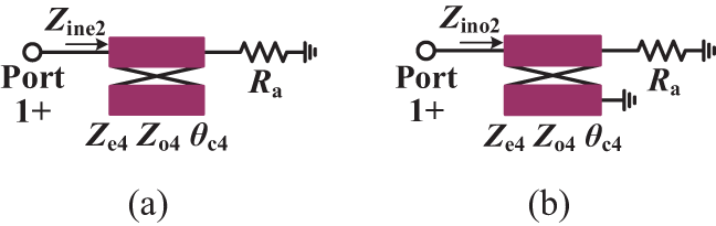
The CM and DM reflectionless balanced BPF is realized by integrating CM and DM reflectionless structures at both the input and output ports of the balanced BPF. Figure 8(a) and 8(b) shows the CM and DM equivalent circuits of CM and DM reflectionless structure (θ c4, R a), respectively. The corresponding input impedances (Z ine2, Z ino2) for the CM and DM equivalent circuit can be derived as follows:
 \begin{equation}{Z_{{\text{ine2}}}} = \frac{{{\text{j}}\left( {{Z_{{\text{e4}}}} + {Z_{{\text{o4}}}}} \right)\,\left( {{Z_{{\text{e4}}}} + {Z_{{\text{o4}}}} - {\text{j2}}{R_{\text{a}}}{\text{cot}}{\theta _{{\text{c4}}}}} \right)}}{{{\text{j4}}{R_{\text{a}}} + {\text{2}}\left( {{Z_{{\text{e4}}}} + {Z_{{\text{o4}}}}} \right)\cot {\theta _{{\text{c4}}}}}}\end{equation}
 \begin{equation}{Z_{{\text{ino2}}}} = \frac{{{\text{2}}{Z_{{\text{e4}}}}{Z_{{\text{o4}}}}\left( \begin{gathered}
{Z_{{\text{e4}}}} + {Z_{{\text{o4}}}} - \hfill \\
{\text{j2}}{R_{\text{a}}}{\text{cot}}{\theta _{{\text{c4}}}} \hfill \\
\end{gathered} \right) + {\text{j}}{R_{\text{a}}}{{\left( {{Z_{{\text{e4}}}} - {Z_{{\text{o4}}}}} \right)}^2}\tan {\theta _{{\text{c4}}}}}}{{{\text{2}}{R_{\text{a}}}\left( {{Z_{{\text{e4}}}} + {Z_{{\text{o4}}}}} \right) - {\text{j4}}{Z_{{\text{e4}}}}{Z_{{\text{o4}}}}\cot {\theta _{{\text{c4}}}}}}\end{equation}
(a) CM equivalent circuit and (b) DM equivalent circuit of the CM and DM reflectionless structure.

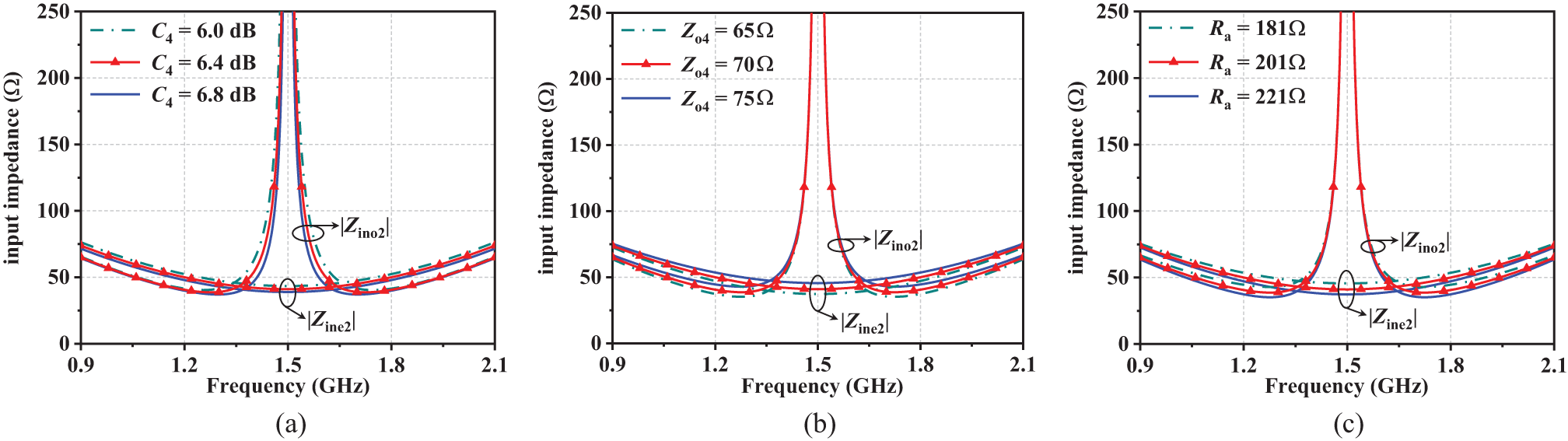
Equations (23) and (24) demonstrate that the input impedances (|Z ine2|, |Z ino2|) are adjustable through proper selection of the coupled line (θ c4) parameters, including characteristic impedance and coupling coefficient, as well as the termination resistance (R a). Figure 9 shows the input impedances of the reflectionless structure for both CM and DM excitations. Under CM excitation, a small offset of |Z ine2| relative to Z 0 = 50 Ω indicates a good impedance match between the CM and DM reflectionless structure and the balanced BPF, meaning an effective CM absorption. Within the passband of the balanced BPF, a high impedance response of the input impedance |Z ino2| indicates that the CM and DM reflectionless structures equivalent to open-circuited, which do not affect the differential filtering performance. Meanwhile, in the out-of-band regions, a small offset of |Z ino2| relative to Z 0 = 50 Ω indicates a good impedance match between the CM and DM reflectionless structure and the balanced BPF under DM excitation, thereby meaning an effective DM absorption. Based on the parameter analysis results shown in Figure 9, a set of reference values for the DM and CM reflectionless balanced BPF is summarized in Table 2.
Variation of the input impedance (Z ine2 and Z ino2): (a) versus different C 4 while fixing Z o4 at 70 Ω, (b) versus different Z o4 while fixing C 4 at 6.4 dB, and (c) versus different R a (C 4 = 6.4 dB, Z o4 = 70 Ω, R a = 201 Ω).

CM and DM reflectionless balanced DM BPF reference values (unit Ω)

In Figure 9(a), the input impedances Z ine2 and Z ino2 are plotted as functions of coupling coefficients C 4, while the odd-mode characteristic impedance Z o4 is fixed at 70 Ω. The results indicate that the high impedance BW of the Z ino2 varies with coupling coefficient C 4. By optimizing the high impedance BW of the Z ino2, a high impedance response can be achieved within the passband of balanced BPF, unaffecting its differential filtering performance. The corresponding mixed-mode S-parameters are illustrated in Figure 10(a). Both wider and narrower high-impedance bandwidths cause deterioration in |S dd11| performances near 1.42 and 1.57 GHz. Figure 9(b) shows that when the coupling coefficient C 4 is fixed at 6.4 dB, both |Z ine2| and |Z ino2| increase with higher Z o4, while the high impedance BW of the |Z ino2| remains relatively stable. Adjusting Z o4 with a fixed C 4 allows simultaneous optimization of reflectionless performance for both CM and DM. The corresponding mixed-mode S-parameters are shown in Figure 10(b). As Z o4 increases, improved absorption characteristics are achieved for both the DM stopband and CM. However, the reflectionless bandwidths are reduced for both DM and CM. The input impedance curves in Figure 9(c) exhibit similar variation trends to those in Figure 9(b), where decreasing R a corresponds to increasing Z o4. The corresponding mixed-mode S-parameters are illustrated in Figure 10(c). To optimize the reflectionless performance for both DM and CM, the design procedure should first adjust the high impedance bandwidth of the Z ino2 by changing C 4, and then changing Z o4 or R a to tune the DM stopband and CM absorption characteristics with reference to Figure 10(b,c) to achieve optimal DM and CM reflectionless performance simultaneously.
Variation of the |S cc11| and |S dd11|: (a) versus different C 4 while fixing Z o4 at 70 Ω, (b) versus different Z o4 while fixing C 4 at 6.4 dB, and (c) versus different R a (C 4 = 6.4 dB, Z o4 = 70 Ω, R a = 201 Ω).

Modulation parameters selection
As illustrated in Figure 1, the time modulated resonators Ri (i = 2, 3) are modulated with varactor diode of Ci(t), as shown as follows:
 \begin{equation}{C_i}\left( t \right) = {C_0} + \Delta C\cos \left[ {{\omega _{\text{m}}}t + \left( {i - 1} \right)\Delta \phi } \right]\quad \left( {i = 1,\;2} \right)\end{equation}
Here ΔC denotes the modulation depth corresponding to the modulation voltage V m, ω m is the modulation angular frequency, and Δφ is the progressive phase shift of the modulation signals [Reference Wu, Liu, Hickle, Peroulis, Gómez-Díaz and Melcón21]. By tuning the modulation parameters, including the modulation frequency f m, modulation voltage V m, and progressive phase shift Δφ, different mixed-mode S-parameter performance can be obtained. To evaluate the influence of these parameters, a comprehensive parametric analysis was conducted with a DC-bias voltage of V dc = 2.86 V applied to each varactor diode. The results are illustrated in Figure 11. A colormap was employed to effectively visualize the parametric analysis results of the forward insertion loss (IL) (|S dd21|) and reverse isolation (|S dd12|), highlighting the variations induced by the modulation parameters. Based on the parametric analysis results, an empirical correlation between the modulation parameters (f m, V m, and Δφ) and the filter specifications (f 0 and FBW, where FBW denotes the fractional bandwidth of the filter without modulation) of the proposed nonreciprocal BPF can be established as follows: f m = 0.8 × FBW × f 0, V m = 20 × FBW, and 80° < ∆φ < 90°.
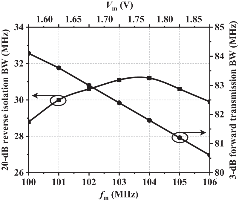
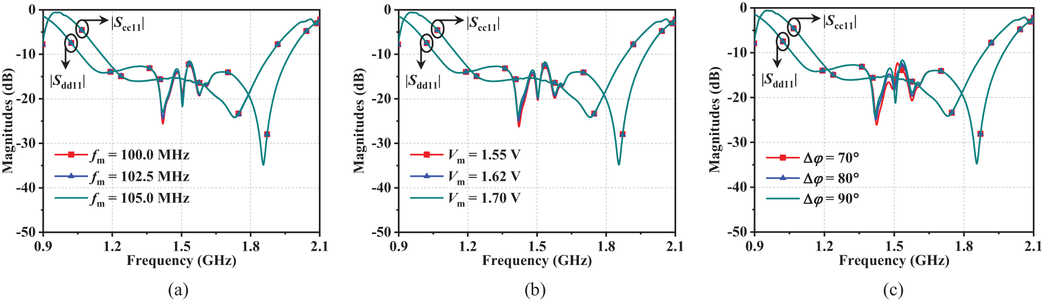
As shown in Figure 11(a), lower f m yield higher reverse isolation but result in smaller 20-dB reverse isolation BW. Figure 11(b) shows that lower V m yield lower forward IL and larger 20-dB reverse isolation BW but result in deteriorated reverse isolation. Form Figure 11(c), larger Δφ values yield higher reverse isolation but result in smaller 20-dB reverse isolation BW. These results demonstrate a trade-off among forward IL, reverse isolation, and reverse isolation BW when selecting modulation parameters. Moreover, Figure 12 shows the variation of 3-dB forward passband and 20-dB reverse isolation BWs with f m and V m. Within a certain frequency range, larger f m values achieve larger 20-dB reverse isolation BW but result in narrower 3-dB forward transmission BW. An optimal trade-off is achieved at the intersection point of these two curves. Furthermore, the DM and CM reflectionless performance remain unaffected by variations in modulation parameters, with corresponding results shown in Figure 13.
Performance variation under different modulation parameters (a) f m, (b) V m, and (c) Δφ.

Variation of 3-dB forward passband and reverse isolation BWs with f m and V m.

Variation of the |S cc11| and |S dd11| under different modulation parameters: (a) f m, (b) V m, and (c) Δφ.

Following the preceding analysis, the proposed design can be implemented through the following design steps: First, based on the performance indicators (e.g., center frequency, BW, and return loss), and combining the mixed-mode S-parameter calculation formulas [Reference Chaudhary and Jeong19] and [Reference Wu and Liu20] with the parameter analysis results shown in Figures 3–6, design the balanced BPF. A fractional bandwidth of 8.4% is a suitable choice for the balanced BPF, with specific parameters adjusted according to Table 1 and Figures 3–6. Next, to achieve CM and DM reflectionless characteristics, CM and DM reflectionless structures are loaded at both the input and output ports of the balanced BPF. The input impedances of these structures are derived from [Reference Simpson and Psychogiou23] and [Reference Alvarez-Melcon, Wu, Zang, Liu and Gomez-Diaz24]. As shown in Figures 9 and 10, the input impedances of the DM/CM reflectionless structures and the mixed-mode S-parameter analysis are presented. Optimal absorption of DM stopband and CM noises occurs when the input impedances Z ine2 for DM stopband and Z ino2 for CM are approximately 50 Ω. Detailed parameter selection can be adjusted based on Tables 1 and 2 and Figures 9 and 10. Subsequently, load the varactor diodes and the compensation microstrip line at the λ-short-circuited resonator to construct the TMR. Figures 11 and 12 show the parametric analysis of the modulation parameters. An empirical correlation of f m = 0.8 × FBW × f 0, V m = 20 × FBW, and 80° < ∆φ < 90° mentioned above. Referring to the parametric analysis shown in Figures 11 and 12 and the empirical correlations, the modulation parameters are tuned to achieve the desired nonreciprocal response within the passband. Finally, considering the substrate parameters, appropriate physical dimensions are selected. A co-simulation approach utilizing ANSYS High-Frequency Structure Simulator (HFSS) and Keysight Advanced Design System (ADS) with large-signal S-parameter analysis is performed to establish the circuit model, ultimately determining the optimized physical dimensions and modulation parameters.
Experimental verification
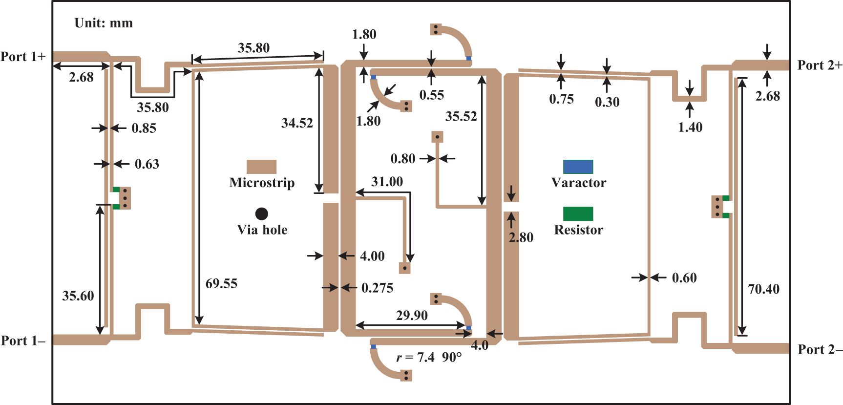
To validate the designed CM and DM reflectionless balanced nonreciprocal BPF, a prototype was fabricated and measured. The prototype was fabricated using F4B dielectric material (ε r = 2.65, tan δ = 0.003) with 1 mm thickness. Figure 14 illustrates the layout and physical dimensions of the fabricated CM and DM reflectionless balanced nonreciprocal BPF. The photographs of the fabricated filter prototype are shown in Figure 15. The fabricated filter prototype was measured using a vector network analyzer (VNA, Agilent Technologies N5230A) connected to its balanced ports (1 ± and 2 ±) via four coaxial lines, and an arbitrary waveform generator (AWG, Tektronix AFG3252C) was connected to the feed ports (Pfeed1, Pfeed2) through two coaxial lines in a back-feeding configuration.
Layout of the proposed CM and DM reflectionless balanced nonreciprocal BPF.

Photographs of the manufactured CM and DM reflectionless balanced nonreciprocal BPF: (a) top view and (b) bottom view.

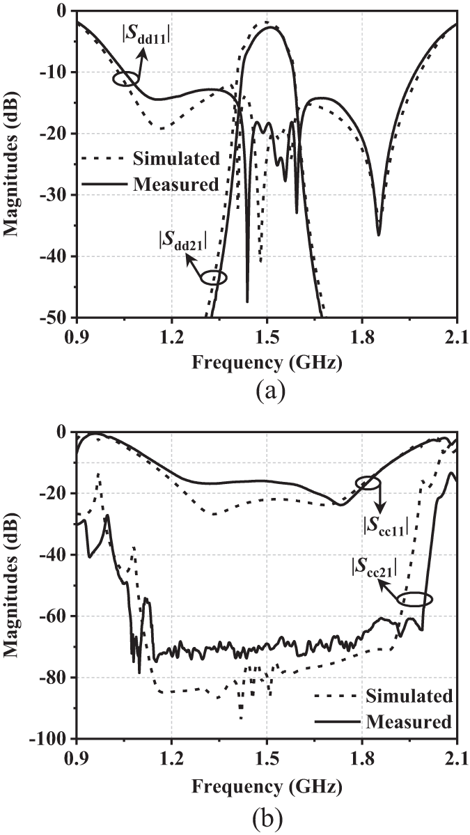
Figure 16 illustrates the simulated and measured responses of the proposed CM and DM reflectionless balanced nonreciprocal BPF under the unmodulated state. Without modulation, the balanced bandpass filter exhibits a reciprocal response with the measured minimum DM insertion loss of 2.7 dB and the measured maximum DM return loss of 18.2 dB in the DM passband. The measured 15-dB CM reflectionless (|S cc11|) BW ranges from 1.23 to 1.83 GHz while the CM suppression (|S cc21|) is better than 60 dB across the 1.14–1.99 GHz range.
Measured results of the proposed CM and DM reflectionless balanced nonreciprocal BPF without modulation: (a) DM responses of |S dd21| and |S dd11| and (b) CM responses of |S cc21| and |S cc11|.

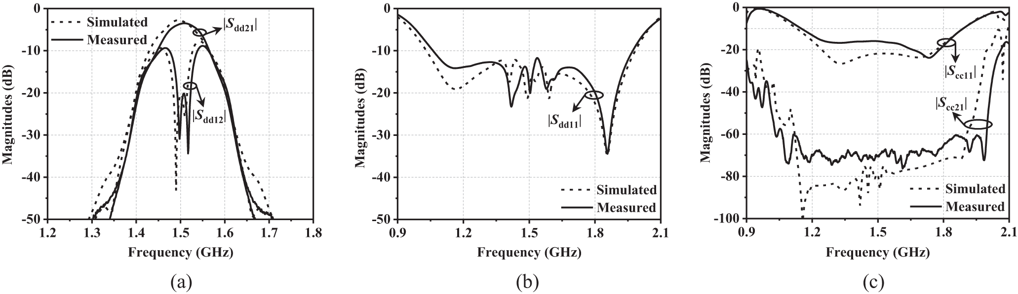
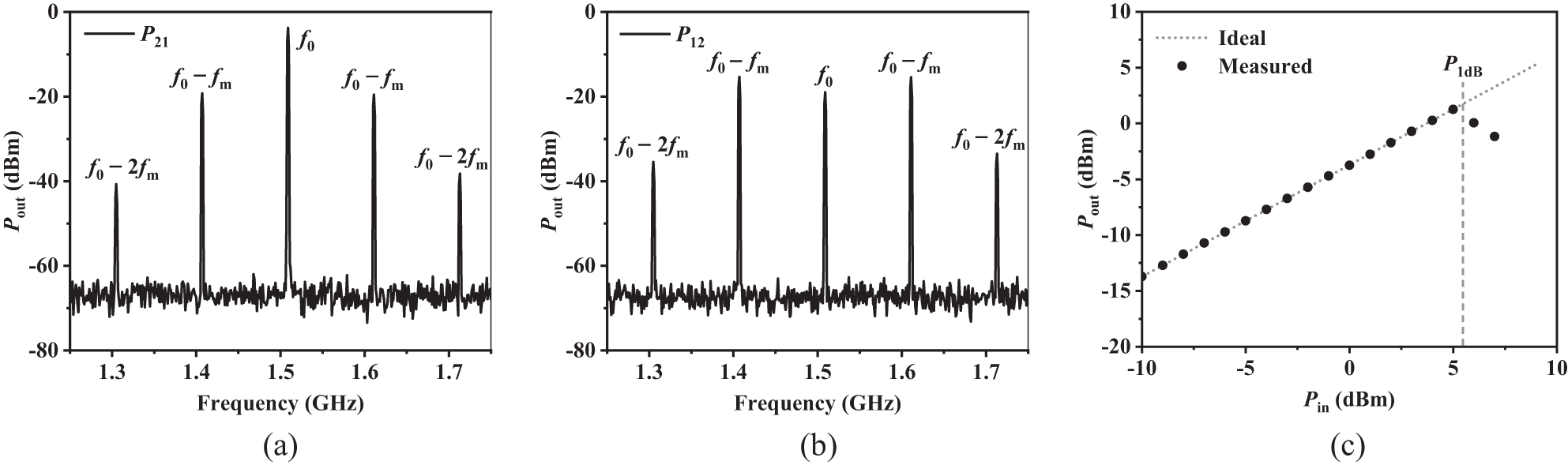
Figure 17 illustrates the simulated and measured responses of the proposed CM and DM reflectionless balanced nonreciprocal BPF under modulated state, demonstrating good agreement. Key parameters of the design are summarized in Table 3 and compared with prior nonreciprocal filter implementations. As shown in Figure 17(a), the minimum DM forward IL (|S dd21|) is measured to be 3.5 dB, with a 3-dB bandwidth (BW3dB) of 84 MHz (from 1.466 to 1.55 GHz), while the 20-dB reverse isolation (|S dd12|) BW is 30.1 MHz. Compared to the unmodulated state, the modulated case exhibits a 0.8-dB degradation in DM forward insertion loss and a 17.3-dB increase in DM reverse isolation. Meanwhile, Figure 17(b) shows that the measured return loss (RL) |S dd11| is better than 10 dB across 1.06–1.97 GHz, achieving a 10-dB DM reflectionless bandwidth of 10.34 × BW3dB. Additionally, Figure 17(c) shows that the measured 15-dB CM reflectionless (|S cc11|) BW spans from 1.23 to 1.83 GHz, achieving a 15-dB CM reflectionless bandwidth of 7.14 × BW3dB. The proposed balanced nonreciprocal BPF achieves a wideband CM and DM reflectionless characteristic. Meanwhile, the 60-dB CM suppression (|S cc21|) BW covers 1.06–1.99 GHz. Figure 18(a) and 18(b) shows the measured output harmonic spectrum of the proposed CM and DM reflectionless balanced nonreciprocal BPF. With a single-tone RF signal (f 0 = 1.509 GHz, P in = 0 dBm) applied to balanced port 1, the output powers at balanced port 2 are −3.76 dBm at f 0 and −19.2/−19.5 dBm at f 0 − f m/f 0 + f m. Conversely, when the same P in is delivered to balanced port 2, the measured output powers at balanced port 1 are −19.0 dBm at f 0 and −15.4 dBm at both f 0 − f m and f 0 + f m. As shown in Figure 18(c), the measured input-referred 1-dB compression point P 1dB at 1.509 GHz is approximately 5.3 dBm.
Measured results of the proposed CM and DM reflectionless balanced nonreciprocal BPF with modulation: (a) DM responses of |S dd21| and |S dd12|, (b) |S dd11|, and (c) CM responses of |S cc21| and |S cc11|.

Measured output harmonic spectrum and input-referred 1-dB compression point of the CM and DM reflectionless balanced nonreciprocal BPF: (a) forward direction P 21 and (b) reverse direction P 12 with a one-tone signal input (f RF = 1.509 GHz and P in = 0 dBm); (c) measured P 1dB.

Comparison between this work and other nonreciprocal filters

Table 3 shows a performance comparison between this work and other nonreciprocal BPFs. The previously reported nonreciprocal BPFs [Reference Alvarez-Melcon, Wu, Zang, Liu and Gomez-Diaz24, Reference Wu, Nafe, Melcón, Gómez-Díaz and Liu28, Reference Chaudhary, Lee, Pech and Jeong29] exhibit poor reverse isolation, while those in [Reference Simpson and Psychogiou22, Reference Simpson and Psychogiou23, Reference Chatzichristodoulou, Arain, Pavlou, Vassiliou, Psychogiou, Nikolaou and Vryonides31, Reference Chaudhary and Jeong32] only achieve high reverse isolation at the center frequency with a narrow 20-dB reverse isolation BW. The works in [Reference Simpson, Vryonides, Nikolaou and Psychogiou39–Reference Han, Wang, Liu and Fang42] focus on balanced nonreciprocal BPFs, offering balanced circuit designs with enhanced immunity to external interference and electromagnetic crosstalk compared to the single-ended nonreciprocal BPFs in [Reference Wu, Liu, Hickle, Peroulis, Gómez-Díaz and Melcón21–Reference Dutta, Kumar and Ram25] and [Reference Chaudhary and Jeong27–Reference Chaudhary and Jeong34]. The design in [Reference Han, Wang, Liu and Fang42] additionally features CM reflectionless characteristics, enabling the absorption of unwanted CM noise and mitigating the adverse effects of radiation emission caused by CM noise. Compared with existing designs, this work is the first to incorporate reflectionless characteristics for both CM and DM signals in the balanced nonreciprocal BPF, at the cost of increased circuit size. It simultaneously achieves in-band backward interference signals isolation and absorbs reflected noise in both CM and DM. Furthermore, a DM reflectionless BW of 10.34 × BW3dB addresses the issue of reflection zero degradation typically observed in time-modulated resonator-based nonreciprocal filters [Reference Wu, Liu, Hickle, Peroulis, Gómez-Díaz and Melcón21–Reference Dutta, Kumar and Ram25, Reference Chaudhary and Jeong27–Reference Chaudhary and Jeong34, Reference Simpson, Vryonides, Nikolaou and Psychogiou39–Reference Han, Wang, Liu and Fang42].
Conclusion
This paper introduces a CM and DM reflectionless balanced nonreciprocal BPF, along with its design methodology and implementation. The reflectionless characteristic is achieved by integrating CM and DM reflectionless structures (two pairs of resistively terminated parallel-coupled lines) at the input and output ports. CM suppression is realized by exploiting the different boundary conditions at the horizontal symmetry plane under DM and CM excitations. Furthermore, two reversely isolated poles are generated by employing two TMRs. The design process combines matrix calculations and parametric studies. The effectiveness of the proposed CM and DM reflectionless balanced nonreciprocal BPF is verified through electromagnetic simulations and physical measurements, with experimental results showing good agreement with simulations. The circuit successfully integrates DM and CM noise absorption, differential filtering, and isolator into a single design. The proposed design is expected to enhance noise immunity and stability in balanced RF circuits.
Acknowledgment
This work was supported by the National Natural Science Foundation of China (No. 61871417), the Liaoning Revitalization Talents Program (No. XLYC2007024), the Natural Science Foundation of Liaoning Province (No. 2019-MS-024), and the Basic Research Project of the Department of Education of Liaoning Province for Universities (No. LJ212410151023).
Competing interests
The authors report no conflict of interest.

Peng Han received the B.Eng. degree in electronic information engineering from Heilongjiang University, China, in 2019. He is currently working toward the Ph.D. degree in information and communication engineering at Dalian Maritime University (DMU). His current research interests include balanced components and nonreciprocal filters.

Zhongbao Wang received the Ph.D. degree in communication and information systems from DMU, China, in 2012. He is currently a Full Professor with the School of Information Science and Technology, DMU. From 2014 to 2018, he was a Postdoctoral Fellow with Beijing University of Posts and Telecommunications, China. From 2019 to 2020, he was a Visiting Scholar with National University of Singapore, Singapore. He has authored more than 100 journal papers. He is currently serving as a Technical Reviewer for the IEEE Trans. on Circuits and Systems, MTT, MWTL, MOTL, and so on. His current research interests include balanced RF components and CP antennas.

Hongmei Liu received the Ph.D. degree in communication and information systems from DMU, China, in 2016. She is currently a Full Professor with the School of Information Science and Technology, DMU. Her current research interests include passive microwave circuits, reconfigurable RF components, and CP microwave antennas.

Shaojun Fang received the Ph.D. degree in communication and information systems from DMU, China, in 2001. Since 1982, he has been at DMU, where he is currently the Head Professor with the School of Information Science and Technology. He has authored or co-authored 4 books and over 120 journal and conference papers. His recent research interests include passive RF components and antennas.