2. Derivation of the general framework

We focus on fully developed CTCFs with both symmetric and asymmetric thermal boundary conditions. The flow is driven by the streamwise body force $F$ and governed by the compressible Navier–Stokes equations

(2.1) \begin{equation} \begin{aligned} \frac {\partial \rho }{\partial t}+\frac {\partial \rho u_j}{\partial x_j} & =0, \\ \frac {\partial \rho u_i}{\partial t}+\frac {\partial \rho u_iu_j}{\partial x_j} & =-\frac {\partial p}{\partial x_i}+\frac {\partial \tau _{ij}}{\partial x_j}+F\delta _{i1}, \\ \frac {\partial \rho E}{\partial t}+\frac {\partial \left [ u_j\left ( \rho E+p \right ) \right ]}{\partial x_j} & =\frac {\partial u_i\tau _{ij}}{\partial x_j}-\frac {\partial q_j}{\partial x_j}+Fu_1, \end{aligned} \end{equation}

with the viscous stress $\tau _{ij}$ and molecular heat flux $q_j$ given as

(2.2) \begin{equation} \tau _{ij}=\mu \left ( \frac {\partial u_i}{\partial x_j}+\frac {\partial u_j}{\partial x_i}-\frac {2}{3}\frac {\partial u_k}{\partial x_k}\delta _{ij} \right ) , \quad q_j=-\lambda \frac {\partial T}{\partial x_j}. \end{equation}

Here, $\delta _{ij}$ denotes the Kronecker delta, and $i=1,2,3$ represent the streamwise ( $x$ ), wall-normal ( $y$ ) and spanwise ( $z$ ) directions, respectively. The fluid is considered as a calorically perfect gas, characterised by the equation of state $p = \rho R T$ , where $p$ , $\rho$ , $R$ and $T$ denote the pressure, density, specific gas constant and temperature, respectively. Also, $u_i$ is the $i$ th velocity component, and $E = e + u_i u_i /2$ is the total energy per unit mass, where $e = c_v T$ is the internal energy, with $c_v = R / (\gamma - 1)$ being the specific heat capacity at constant volume, and $\gamma = c_p / c_v = 1.4$ the specific heat ratio. The dynamic viscosity $\mu$ follows Sutherland’s law or the power law $\mu \propto T^{0.7}$ (Lusher & Coleman Reference Lusher and Coleman2022), and the thermal conductivity is given by $\lambda = \mu c_p / Pr$ , with a constant Prandtl number.

Figure 1.

Illustrations of CTCFs with (a) symmetric and (b) asymmetric thermal boundary conditions.

As shown in figure 1, periodic boundary conditions are applied in the streamwise and spanwise directions, while no-slip conditions are imposed for velocity at the walls. In the symmetric case, both walls are maintained at the same temperature $T_w$ (Yao & Hussain Reference Yao and Hussain2020; Zhang & Xia Reference Zhang and Xia2020; Zhang, Song & Xia Reference Zhang, Song and Xia2023). In the asymmetric case, the lower wall is fixed at $T_{w,L}$ , while the upper wall is either adiabatic ( $\partial T / \partial y = 0$ ) (Lusher & Coleman Reference Lusher and Coleman2022) or fixed at $T_{w,H}$ (Zhang, Song & Xia Reference Zhang, Song and Xia2024). In the following, both Reynolds averaging $\phi = \bar \phi + \phi ^{\prime }$ and Favre averaging $\phi = \tilde \phi + \phi ^{\prime \prime }$ are employed to decompose the quantity $\phi$ into its mean and fluctuating components. The friction velocity $u_\tau = \sqrt {\bar \tau _w / \bar \rho _w}$ (where $\bar \tau _w = \left . \bar \tau _{12} \right |_w$ is the wall shear stress) and the viscous length scale $\delta _\nu = \bar \mu _w / (\bar \rho _w u_\tau )$ characterise the inner scaling with a superscript +, while the semi-local friction velocity $u_\tau ^* = \sqrt {\bar \tau _w / \bar \rho }$ and viscous length scale $\delta _\nu ^* = \bar \mu / (\bar \rho u_\tau ^*)$ define the semi-local scaling with a superscript *.

The integral of the Reynolds-averaged momentum and total energy equations in (2.1) reveals the balance between molecular and turbulent diffusion fluxes (Huang, Coleman & Bradshaw Reference Huang, Coleman and Bradshaw1995):

(2.3) \begin{equation} \bar {\mu }\,\frac {{\mathrm{d}}\tilde {u}}{{\mathrm{d}}y}-\bar {\rho }\,\widetilde {u^{\prime \prime }v^{\prime \prime }} \approx \bar \tau _w -\int _0^y\bar {F}\,{\mathrm{d}}y \end{equation}

and

(2.4) \begin{equation} \bar {\mu }\,\frac {{\mathrm{d}}\tilde {K}}{{\mathrm{d}}y}-\bar {\rho }\,\widetilde {K^{\prime \prime }v^{\prime \prime }}+\bar {\mu }\,\frac {{\mathrm{d}}\tilde {k}}{{\mathrm{d}}y}-\bar {\rho }\,\widetilde {k^{\prime \prime }v^{\prime \prime }}+\bar {\lambda }\,\frac {{\mathrm{d}}\tilde {T}}{{\mathrm{d}}y}-c_p\bar {\rho }\,\widetilde {T^{\prime \prime }v^{\prime \prime }} \approx -\bar q_w - \int _0^y{\overline {Fu}}\,{\mathrm{d}}y. \end{equation}

Here, $\bar \tau _t = \bar \mu\, {\mathrm{d}}\tilde u / {\mathrm{d}}y - \bar \rho\, \widetilde {u^{\prime \prime }v^{\prime \prime }}$ is the total shear stress, and $\bar q_w = \left . \bar q_2 \right |_w$ is the wall heat flux. The decomposition of the instantaneous kinetic energy, $u_iu_i/2 = \tilde K + K^{\prime \prime } + \tilde k + k^{\prime \prime }$ , is introduced to simplify $\overline {\tau _{i2}u_i}$ , where $\tilde K = \tilde u_i \tilde u_i / 2$ , $K^{\prime \prime } = \tilde u_i u_i^{\prime \prime }$ , $\tilde k = \widetilde {u_i^{\prime \prime }u_i^{\prime \prime }}/2$ and $k^{\prime \prime } = u_i^{\prime \prime }u_i^{\prime \prime }/2 - \widetilde {u_i^{\prime \prime }u_i^{\prime \prime }}/2$ (Huang et al. Reference Huang, Coleman and Bradshaw1995, Reference Huang, Coleman, Spalart and Yang2023). Additionally, the molecular diffusion flux of a quantity $\phi$ , $\overline {\mu\, {\mathrm{d}}\phi /{\mathrm{d}}y}$ , is approximated by its dominant term $\bar \mu\, {\mathrm{d}}\tilde {\phi }/{\mathrm{d}}y$ during the above derivation.

Following previous studies (Zhang et al. Reference Zhang, Bi, Hussain and She2014; Huang et al. Reference Huang, Coleman, Spalart and Yang2023; Cheng & Fu Reference Cheng and Fu2024a ), the quasi-parallel flow approximation $u_i u_i \approx u^2$ and small turbulence approximation $u^2 \approx \tilde u^2 + 2\tilde u u^{\prime \prime }$ are further adopted. These approximations are intended to exclude higher-order terms, commonly absent in open-source DNS data, thereby preserving the simplicity of turbulence modelling. However, they do introduce some non-negligible effects on accuracy, such as $\overline {\tau _{i2}u_i} \approx \bar {\mu } \tilde {u}\, {\mathrm{d}}\tilde {u}/{\mathrm{d}}y$ near the adiabatic wall, as detailed by Cheng & Fu (Reference Cheng and Fu2024a ) and in Appendix A. Anyway, the total heat flux equation can then be derived by combining (2.3) and (2.4) while assuming $\overline {Fu} = \bar F \tilde u$ :

(2.5a) \begin{align}&\,\, {\bar {q}_t = -\left ( \bar {\lambda }+\bar {\lambda }_t \right ) \frac {{\mathrm{d}}\tilde {T}}{{\mathrm{d}}y}=\bar {q}_w + \int _0^y{\bar {\tau }_{12}\frac {{\mathrm{d}}\tilde {u}}{{\mathrm{d}}y}\,{\mathrm{d}}y}+\int _0^y{\bar {R}_{12}\frac {{\mathrm{d}}\tilde {u}}{{\mathrm{d}}y}\,{\mathrm{d}}y}, } \end{align}

(2.5b) \begin{align}& {\bar {q}_t = -\left ( \bar {\lambda }+\bar {\lambda }_t \right ) \frac {{\mathrm{d}}\tilde {T}}{{\mathrm{d}}y}= \bar {q}_{t,e} - \int _y^{\delta _e}{\bar {\tau }_{12}\frac {{\mathrm{d}}\tilde {u}}{{\mathrm{d}}y}\,{\mathrm{d}}y}-\int _y^{\delta _e}{\bar {R}_{12}\frac {{\mathrm{d}}\tilde {u}}{{\mathrm{d}}y}\,{\mathrm{d}}y}.} \end{align}

It is important to note that (2.5a ) and (2.5b ) represent the forms integrated from the wall ( $y = 0$ ) and the effective boundary layer edge ( $y = \delta _e$ , where ${\mathrm{d}}\tilde {u} / {\mathrm{d}}y = 0$ ), respectively. Here, $\bar \lambda _t = - c_p \bar \rho\, \widetilde {T^{\prime \prime }v^{\prime \prime }} / ({\mathrm{d}}\tilde T/{\mathrm{d}}y)$ is the eddy thermal conductivity, $\bar \tau _{12} = \bar \mu\, {\mathrm{d}}\tilde u / {\mathrm{d}}y$ is the mean viscous shear stress, and $\bar R_{12} = -\bar \rho\, \widetilde {u^{\prime \prime }v^{\prime \prime }}$ is the turbulent shear stress. Additionally, $\bar {q}_{t,e} = ( -\bar \lambda\, {{\mathrm{d}}\tilde T}/{{\mathrm{d}}y} + c_p \bar {\rho }\, \widetilde {T^{\prime \prime }v^{\prime \prime }} ) |_e$ denotes the mean total heat flux at the effective boundary layer edge $y = \delta _e$ . The physical significance is clear: for instance, (2.5a ) indicates that the difference between the total heat flux $\bar {q}_t(y)$ and wall heat flux $\bar {q}_w$ arises from the production of turbulent kinetic energy and molecular viscous dissipation within the control volume $[0, y]$ . Notably, unlike previous approaches (Chen et al. 2022a; Huang et al. Reference Huang, Coleman, Spalart and Yang2023; Cheng & Fu Reference Cheng and Fu2024a ), the constant-stress layer approximation $\bar \tau _t \approx \bar \tau _w$ has not been applied directly.

Inspired by the derivation of Walz’s equation (Walz Reference Walz1969; Smits & Dussauge Reference Smits and Dussauge2006; Zhang et al. Reference Zhang, Bi, Hussain and She2014), we introduce the eddy viscosity $\bar {\mu }_t = -\bar {\rho }\, \widetilde {u^{\prime \prime } v^{\prime \prime }} / ({\mathrm{d}}\tilde {u} / {\mathrm{d}}y)$ and the mixed Prandtl number $Pr_m = c_p (\bar {\mu } + \bar {\mu }_t) / (\bar {\lambda } + \bar {\lambda }_t)$ , while acknowledging that $\tilde T = \tilde T(\tilde u)$ . Subsequently, $\bar {\rho }_w c_p u_\tau \tilde {T}_w$ is divided out from both sides of (2.5a ) and (2.5b ), leading to their dimensionless forms as

(2.6a) \begin{align}&\,\, {\frac {\bar {\tau }_{t}^{+}}{Pr_m}\,\frac {{\mathrm{d}}\theta }{{\mathrm{d}}\tilde {u}^+} =B_q+\left ( \gamma -1 \right ) M_{\tau }^{2}\int _0^{\tilde {u}^+}{\bar {\tau }_{t}^{+}}\,{\mathrm{d}}\tilde {u}^+,\quad \left . \theta \right |_{w} = 0}, \end{align}

(2.6b) \begin{align}& {\frac {\bar {\tau }_{t}^{+}}{Pr_m}\,\frac {{\mathrm{d}}\theta }{{\mathrm{d}}\tilde {u}^+}=Q_{t,e}-\left ( \gamma -1 \right ) M_{\tau }^{2}\int _{\tilde {u}^+}^{\tilde {u}_{e}^{+}}{\bar {\tau }_{t}^{+}}\,{\mathrm{d}}\tilde {u}^+,\quad \left . \theta \right |_{w} = 0}, \end{align}

where $B_q = \bar q_w / (\bar \rho _w c_p u_\tau \tilde T_w)$ is the dimensionless wall heat flux, $M_\tau = u_\tau / \sqrt {\gamma R \tilde T_w}$ is the friction Mach number, $Q_{t,e} = \bar q_{t,e} / (\bar \rho _w c_p u_\tau \tilde T_w)$ is the dimensionless total heat flux at the effective boundary layer edge, and $\tilde u_e$ is the mean velocity at the effective boundary layer edge. The dimensionless mean temperature $\theta = 1 - \tilde T / \tilde T_w$ can be determined directly by integrating (2.6a ), provided that $B_q, M_\tau , \bar \tau _t^+, \tilde u^+, Pr_m$ are known:

(2.7) \begin{equation} \begin{aligned} \theta (B_q, M_\tau ,\bar \tau _t^+,\tilde u^+,Pr_m) &= \int _0^{\tilde {u}^+} \frac {Pr_m}{\bar {\tau }_{t}^{+}} f(B_q, M_\tau ,\bar \tau _t^+,\tilde u^+) \, {\mathrm{d}}\tilde {u}^+, \\ f(B_q, M_\tau ,\bar \tau _t^+,\tilde u^+) &= B_q + (\gamma - 1) M_{\tau }^{2} \int _0^{\tilde {u}^+} \bar {\tau }_{t}^{+} \, {\mathrm{d}}\tilde {u}^+. \end{aligned} \end{equation}

In the constant-stress layer of high Reynolds number flows, where $y/\delta _e \ll 1$ , the approximation $\bar \tau _t^+ \approx 1$ is typically adopted, simplifying (2.7) to

(2.8) \begin{equation} \theta (B_q, M_\tau ,\tilde u^+,Pr_m) =\int _0^{\tilde {u}^+}{Pr_m\left [ B_q+\left ( \gamma -1 \right ) M_{\tau }^{2}\tilde {u}^+ \right ]}{\mathrm{d}}\tilde {u}^+. \end{equation}

If $Pr_m \approx Pr$ is further adopted in the near-wall region ( $y^* \lesssim 5$ ), then a quadratic relationship between the mean temperature and mean velocity can be given as (Huang & Coleman Reference Huang and Coleman1994)

(2.9) \begin{equation} \theta (B_q, M_\tau ,\tilde u^+,Pr) =Pr\,B_q\tilde {u}^++\left ( \gamma -1 \right ) M_{\tau }^{2}\frac {Pr}{2}\tilde {u}^{+2}. \end{equation}

In CTCFs, $\bar \tau _t^+$ can be derived theoretically from the mean streamwise momentum equation. Consequently, (2.7)–(2.9) can be interpreted as the mean temperature–velocity relation and its two approximations, when $Pr_m$ is appropriately modelled. The two key wall parameters, $B_q$ and $M_\tau$ , make them potentially applicable across a wide range of wall thermodynamic conditions and Mach numbers. Additionally, it is worth noting that the mean temperature–velocity relation derived by Huang, Bradshaw & Coakley (Reference Huang, Bradshaw and Coakley1993), Huang & Coleman (Reference Huang and Coleman1994)and Huang et al. (Reference Huang, Coleman, Spalart and Yang2023) can be regarded as a special case of (2.8) in the logarithmic layer, where $Pr_m \approx Pr_t \approx \kappa / \kappa _T \approx 0.85$ .

3. The modelling of $Pr_m$

Drawing on the DNS data from Abe & Antonia (Reference Abe and Antonia2019) and Lluesma-Rodríguez et al. (Reference Lluesma-Rodríguez, Hoyas and Perez-Quiles2018), Huang et al. (Reference Huang, Coleman, Spalart and Yang2023) demonstrated that $Pr_m(y^+)$ ( $Pr_{total}$ in their paper) exhibits an excellent collapse at $y^+ \lesssim 10$ , attains peak value approximately 1 at $y^+ \approx 50$ , and levels off at 0.85 for $y^+ \gtrsim 150$ in flows with $Re_\tau \gt 1000$ . Meanwhile, a similar trend was observed in the semi-local coordinate $y^*$ using the compressible DNS data provided by Lusher & Coleman (Reference Lusher and Coleman2022). Consequently, they extended the incompressible $Pr_m$ model to compressible flows by assuming the Mach independence of $Pr_m(y^*)$ . Nonetheless, in order to minimise the number of empirical parameters while maintaining simplicity, we prefer employing a damping function to directly capture the universal profile of $Pr_m(y^*)$ before its peak, i.e.

(3.1) \begin{equation} Pr_m(y^*)=Pr+\left ( 1-Pr \right ) D_{Pr_m}^{*}, \quad D_{Pr_m}^{*}(y^*) =\left [ 1-\exp \left ( -{y^*}/{A_{Pr_m}^{*}} \right ) \right ] ^n. \end{equation}

The empirical parameters $A_{Pr_m}^* = 10$ and $n=3$ are obtained by fitting the DNS data from Lusher & Coleman (Reference Lusher and Coleman2022), including the $Pr_m(y^*)$ profiles on both the isothermal cold wall and adiabatic hot wall sides at $y^* \leqslant 50$ . The present model is thoroughly compared with both DNS data and the model proposed by Huang et al. (Reference Huang, Coleman, Spalart and Yang2023), as shown in figure 2. It is apparent that our model shows significant improvement before the peak, which dominates the accuracy of (2.7). While Huang’s model remains effective post-peak, we have decided to abandon such modelling. The implications and justification for this simplification will be discussed in the next section and Appendix A.

Figure 2.

Comparison of the performance of (3.1) (black solid lines) with Huang’s model (grey solid lines) for modelling $Pr_m(y^*)$ , in both symmetric and asymmetric CTCFs, with (a) $Pr = 0.7$ (Lusher & Coleman Reference Lusher and Coleman2022) and (b) $Pr = 0.72$ (Zhang & Xia Reference Zhang and Xia2020; Zhang et al. Reference Zhang, Song and Xia2023, Reference Zhang, Song and Xia2024). The definitions of the labels are provided in § 4.

Additionally, special attention should be given to the fact that the proposed model implies $Pr_m - Pr = \mathcal{O}(y^{*3})$ as $y^* \rightarrow 0$ , which does not align with the asymptotic behaviour at the wall under various thermal boundary conditions. For instance, in incompressible wall-bounded turbulence with constant properties, asymptotic analysis reveals that while the proposed model satisfies the imposed temperature boundary condition, it fails to account for adiabatic and imposed heat flux conditions. Although not shown here, this discrepancy can be observed for $y^* \lesssim 3$ when using a log-log scale instead of a semi-logarithmic scale. Undoubtedly, a more accurate, physics-informed model would be preferable, necessitating a detailed investigation of the behaviour of $Pr_m$ both near the wall and beyond its peak. The current model serves as a temporary compromise, and future studies are expected to further refine and improve it.

4. Verification and evaluation

In this section, DNS data of CTCFs are employed to systematically evaluate the mean temperature–velocity relation derived from the GRA theory, as given in (1.1), where $\tilde T_e$ is obtained from the DNS data, alongside the proposed relations in (2.7)–(2.9), with $Pr_m$ determined by (3.1). The dataset encompasses symmetric cases with isothermal walls from Yao & Hussain (Reference Yao and Hussain2020), Zhang & Xia (Reference Zhang and Xia2020) and Zhang et al. (Reference Zhang, Song and Xia2023), as well as those with asymmetric thermal boundary conditions from Lusher & Coleman (Reference Lusher and Coleman2022) and Zhang et al. (Reference Zhang, Song and Xia2024). For clarity, all cases are relabelled in this paper. For instance, ‘M15R6KT32L(H)’ refers to the flow region near the lower cold (upper hot) wall, with bulk Mach number $M_b = 1.5$ , bulk Reynolds number $Re_b = 6000$ , and wall temperature ratio between the upper hot and lower cold wall of $\tilde {T}_{w,H} \approx 3.2 \tilde {T}_{w,L} = 3.2T_{ref}$ .

Figure 3.

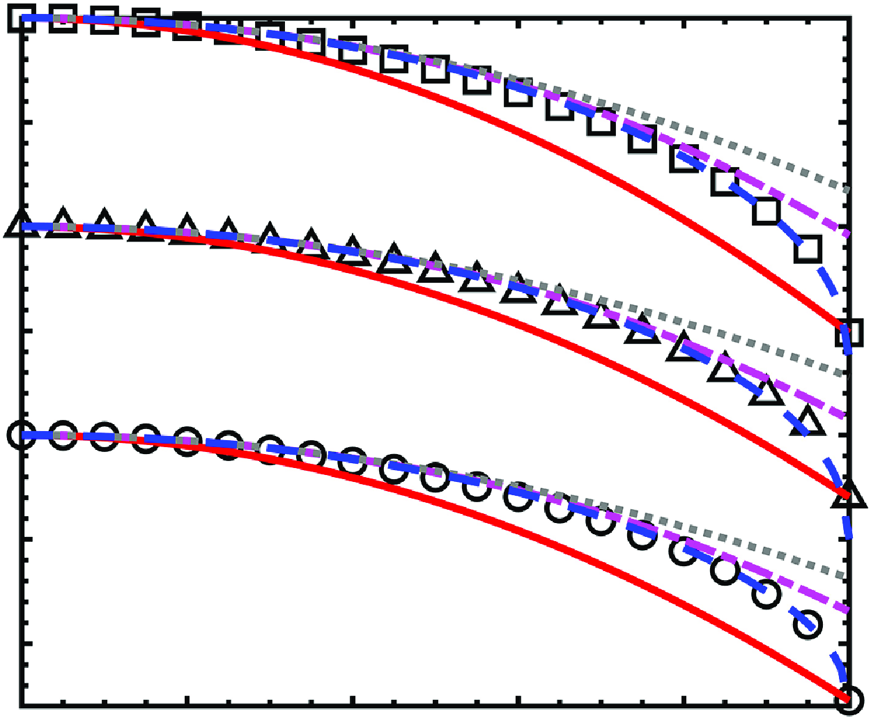
Comparison of DNS data for symmetric cases (symbols) with various mean temperature-velocity relations: (1.1) (red solid lines), (2.7) (blue dashed lines), (2.8) (pink dash-dotted lines) and (2.9) (grey dotted lines). The datasets are sourced from (a) Zhang & Xia (Reference Zhang and Xia2020) and Zhang et al. (Reference Zhang, Song and Xia2023), and (b) Yao & Hussain (Reference Yao and Hussain2020). For clarity, the results in (b) are shifted upwards.

In channels with symmetric isothermal walls, the total shear stress is $\bar \tau _t^+ = 1 - y/h$ when the flow is driven by a uniform body force. To derive $\tilde T / \tilde T_w = 1 - \theta$ via (2.7), $B_q$ , $M_\tau$ , $\tilde u^+$ , $y/h$ , $y^*$ and $Pr$ are required. Figure 3 provides a comprehensive comparison of the proposed mean temperature–velocity relation and its approximations (2.7)–(2.9), alongside the GRA relation (1.1). As observed, the GRA relation and the proposed one demonstrate nearly equivalent performance, with the former showing a slight advantage as $\tilde {u}/\tilde {u}_e \rightarrow 1$ due to $\tilde T_e$ being directly constrained by DNS data. The constant-stress layer assumption and the approximation $Pr_m \approx Pr$ , i.e. (2.8) and (2.9), further limit the model’s utility to the inner layer and the near-wall region, respectively. It is noteworthy that (2.7) preserves the GRA relation’s efficacy across varying Mach numbers (figure 3 a) and Reynolds numbers (figure 3 b), with their discrepancies from DNS data primarily attributed to the omission of higher-order terms in deriving (2.5) (see Appendix A for details).

Figure 4.

Comparison of DNS data for asymmetric cases (symbols) with various mean temperature–velocity relations. The equations corresponding to different line types are the same as those in figure 3. The datasets are sourced from Lusher & Coleman (Reference Lusher and Coleman2022) and Zhang et al. (Reference Zhang, Song and Xia2024). Plots in (a) and (b) show results within the boundary layers adjacent to the lower cold and upper hot walls, respectively, with upward shifts applied for clarity.

In channel flows with asymmetric thermal boundary conditions, the total shear stress is given by $\bar \tau _{t}^+ = 1 - y / \delta _{e}$ for each wall side, when the flow is driven by a uniform body force. In this context, $B_q, M_\tau , \tilde u^+, y/\delta _{e}, y^*, Pr$ are needed to derive $\tilde T / \tilde T_w$ via (2.7). As shown in figure 4, the GRA relation fails on both the cold lower and hot upper wall sides. In contrast, the proposed model is in close agreement with DNS data across various $M_b$ , $Re_b$ and $\tilde T_{w,H} / \tilde T_{w,L}$ , especially in capturing the behaviour of $ {\mathrm{d}}\tilde T / {\mathrm{d}} \tilde u |_e \rightarrow \infty$ , which cannot be characterised by the quadratic relation provided in (1.1). Furthermore, the two associated approximations (2.8) and (2.9) continue to be applicable within their specific regions.

Figure 5.

Integrated percentage errors of the mean temperature–velocity relations (1.1) (open symbols) and (2.7) (closed symbols) applied to (a) 14 profiles from symmetric cases, and (b) 16 profiles from asymmetric cases. The symbols , , and represent DNS data from Zhang et al. (Reference Zhang, Song and Xia2023), Yao & Hussain (Reference Yao and Hussain2020), Zhang et al. (Reference Zhang, Song and Xia2024), and Lusher & Coleman (Reference Lusher and Coleman2022), respectively.

For more quantitative assessments, the integrated percentage error is defined as

(4.1) \begin{equation} \varepsilon ( \% ) =\frac {\int _0^{\tilde {u}_e}{\left | ( \tilde {T}/\tilde {T}_w ) _{pre}-( \tilde {T}/\tilde {T}_w ) _{data} \right |\,{\mathrm{d}}( \tilde {u}/\tilde {u}_e )}}{\int _0^{\tilde {u}_e}{ (\tilde {T}/\tilde {T}_w ) _{data}\,{\mathrm{d}}( \tilde {u}/\tilde {u}_e )}}\times 100\,\%, \end{equation}

where $( \tilde {T}/\tilde {T}_w )_{data}$ and $\tilde u / \tilde u_e$ are obtained from the DNS data, while $( \tilde {T}/\tilde {T}_w )_{pre}$ is predicted by the GRA relation and the proposed one, (1.1) and (2.7), respectively. The results are presented in figure 5. It can be clearly seen that the proposed model achieves accuracy that is nearly on a par with, or slightly inferior to, the GRA relation in symmetric cases, with all errors remaining below 2 %. Additionally, the present model shows a notable improvement when dealing with asymmetric thermal boundary conditions, with the majority of errors less than 1 %, in contrast to the GRA relation where all errors exceed 2 %. Notably, we also found that using either DNS data or the proposed model to determine $Pr_m$ does not significantly impact the mean temperature profiles (see Appendix A for details), thus indirectly confirming the effectiveness of (3.1). Furthermore, the results demonstrate that the integrated percentage error increases with the bulk Mach number at a fixed characteristic Reynolds number $Re_\tau ^*$ . Since the proposed relation exhibits a trend consistent with the GRA relation, we attribute this to the degradation of the same approximations underlying their derivations. For instance, the neglected fluctuating component in the approximation of the molecular diffusion flux (i.e. $\overline {\mu\, {\mathrm{d}}\phi /{\mathrm{d}}y} \approx \bar \mu\, {\mathrm{d}}\tilde \phi / {\mathrm{d}}y$ ) becomes increasingly significant as compressibility effects intensify.

5. Further discussions and applications

5.1. Mean temperature decomposition and the modified GRA relation

Zhang et al. (Reference Zhang, Bi, Hussain and She2014) have demonstrated that the GRA relations $\tilde H_g - \tilde H_w = U_w \tilde u$ and $H_g^{\prime \prime } + c_p \phi ^{\prime \prime } = U_w u^{\prime \prime }$ (where $H_g = c_p T + r_g u^2/2$ is the general recovery enthalpy, $\phi ^{\prime \prime }$ denotes the residual temperature fluctuations, and $U_w = c_p\, \partial \tilde T / \partial \tilde u |_w$ ) can be admitted as similarity solutions by substituting them into the mean momentum and energy equations. By following a similar procedure, it can be derived that

(5.1) \begin{equation} \frac {{\mathrm{d}}}{{\mathrm{d}}y}\left ( \bar {\mu }\frac {{\mathrm{d}}\tilde {\chi }}{{\mathrm{d}}y} \right ) =0, \end{equation}

for CTCFs, where $\tilde \chi = \tilde H_g - \tilde H_w - U_w\tilde u$ . Meanwhile, the boundary conditions are given by

(5.2) \begin{equation} \begin{cases} y =0, & \tilde {\chi }=0, \\ y =\delta _e, & \dfrac {{\mathrm{d}}\tilde {\chi }}{{\mathrm{d}}y}= \left . c_p\dfrac {{\mathrm{d}}\tilde {T}}{{\mathrm{d}}y} \right |_e + \dfrac {\tilde {u}_e^2}{2} \left .\dfrac {{\mathrm{d}} r_g}{{\mathrm{d}} y}\right |_e. \end{cases} \end{equation}

It should be noted that (1.1) is derived under the assumption that the effective turbulent Prandtl number is $Pr_e = 1$ , which implies ${\mathrm{d}}r_g / {\mathrm{d}}y = 0$ . For channels with symmetric isothermal walls, it is straightforward to conclude that (5.1) and (5.2) permit the GRA relation $\tilde \chi = 0$ as ${\mathrm{d}}\tilde T / {\mathrm{d}}y = 0$ at the channel centre. However, such a solution is denied for cases with asymmetric thermal boundary conditions due to non-zero total heat flux at the boundary layer edge, despite complying with the governing equation and wall boundary conditions. This is the intrinsic reason why (1.1) is highly effective in symmetric cases yet inadequate for asymmetric cases, as evidenced in § 4.

By analysing (2.6b ) and the results from § 4, it can be inferred that the GRA relation effectively describes the mean temperature component arising from turbulence production and viscous dissipation, but fails to account for the portion induced by $Q_{t,e} \neq 0$ . To address this issue, we introduce a decomposition of the mean temperature into its ‘pure’ and ‘residual’ components, $\tilde T = \tilde T_{pure} + \tilde T_{res}$ , where $\tilde T_{pure}$ is expected to be characterised by the GRA relation, and $\tilde T_{res}$ accounts for the physics of asymmetry. By introducing $\theta _{pure} = 1 - \tilde T_{pure} / \tilde T_w$ and $\theta _{res} = -\tilde T_{res} / \tilde T_w = \theta - \theta _{pure}$ , (2.6b ) can be separated into

(5.3) \begin{equation} \frac {\bar {\tau }_{t}^{+}}{Pr_m}\,\frac {{\mathrm{d}}\theta _{pure}}{{\mathrm{d}}\tilde {u}^+}=-\left ( \gamma -1 \right ) M_{\tau }^{2}\int _{\tilde {u}^+}^{\tilde {u}_{e}^{+}}{\bar {\tau }_{t}^{+}}\,{\mathrm{d}}\tilde {u}^+,\quad \left . \theta _{pure} \right |_{w}=0, \end{equation}

and

(5.4) \begin{equation} \frac {\bar {\tau }_{t}^{+}}{Pr_m}\,\frac {{\mathrm{d}}\theta _{res}}{{\mathrm{d}}\tilde {u}^+}=Q_{t,e},\quad \left . \theta _{res} \right |_{w}=0. \end{equation}

By replacing the mean temperature $\tilde T$ with its ‘pure’ component $\tilde T_{pure}$ , it can be demonstrated that the modified GRA relation, $\tilde H_{g,m} - \tilde H_{w} = U_{w,m} \tilde u$ and $H_{g,m}^{\prime \prime } + c_p \phi ^{\prime \prime } = U_{w,m}u^{\prime \prime }$ , is compatible with both the mean momentum and energy equations, as well as the associated boundary conditions. Therefore, the modified version of (1.1) can be expressed as

(5.5) \begin{equation} \frac {\tilde {T}_{pure}}{\tilde {T}_{w}}=1+\frac {\tilde {T}_{rg,m}-\tilde {T}_{w}}{\tilde {T}_{w}}\frac {\tilde {u}}{\tilde {u}_e}+\frac {\tilde {T}_{pure,e}-\tilde {T}_{rg,m}}{\tilde {T}_{w}}\left ( \frac {\tilde {u}}{\tilde {u}_e} \right ) ^2, \end{equation}

where $\tilde T_{rg,m} = \tilde T_{pure,e} + r_{g,m} \tilde u_e^2 / (2 c_p)$ and $r_{g,m} = 2c_p (\tilde T_{w} - \tilde T_{pure,e}) / \tilde u_e^2 + 2 c_p / \tilde u_e \times {\mathrm{d}}\tilde T_{pure} / {\mathrm{d}}\tilde u |_w$ .

Figure 6.

(a,b) Wall-normal distributions of the mean temperature ratio $\tilde T / \tilde T_w$ (symbols), along with the two components $\tilde T_{pure} / \tilde T_{w}$ (solid lines) and $\tilde T_{res} / \tilde T_w + 1$ (dashed lines). (c,d) Comparison of DNS data for $\tilde T_{pure} / \tilde T_{w}$ (symbols) with the modified GRA relation (5.1) (red solid lines). The data are from Lusher & Coleman (Reference Lusher and Coleman2022) and Zhang et al. (Reference Zhang, Song and Xia2024). Plots in (a,c) and (b,d) show results within the flow regions adjacent to the lower cold and upper hot walls, respectively, with upward shifts applied in (c,d) for clarity.

Figure 6(a,b) present the results of the proposed mean temperature decomposition, where $1 + \tilde T_{res} / \tilde T_{w}$ is computed directly from DNS data and (5.4), while $\tilde T_{pure} / \tilde T_{w}$ is obtained by subtracting $\tilde T_{res} / \tilde T_{w}$ from $\tilde T / \tilde T_w$ . As expected, the ‘pure’ component exhibits trends similar to those observed in symmetric cases, with a steep gradient near the wall that levels off in the bulk region. Meanwhile, the ‘residual’ component represents the additional mean temperature distribution induced by a constant total heat flux within the boundary layer, $\bar q_{t,res} = -(\bar {\lambda }+\bar {\lambda }_t)\, {{\mathrm{d}}\tilde {T}_{res}}/{{\mathrm{d}}y} = \bar q_{t,e}$ , which is the intrinsic reason for the nearly linear profile of $\tilde T$ in the bulk region, as reported by Zhang et al. (Reference Zhang, Song and Xia2024). These findings provide valuable insights into the effects of asymmetric wall temperature. Moreover, the validity of (5.5) is demonstrated in figure 6 (c,d), which is essentially equivalent to that in symmetric cases.

5.2. Mean temperature transformations

In this subsection, we briefly discuss another application of the total heat flux equation (2.6) for deriving mean temperature transformations, akin to using the total shear stress equation to derive mean velocity transformations (Hasan et al. Reference Hasan, Larsson, Pirozzoli and Pecnik2023; Zhu et al. Reference Zhu, Song, Yang and Xia2024).

Based on (2.6a ), the total heat flux equation for the compressible state is expressed as

(5.6) \begin{equation} \frac {{\bar {\tau }_{t,com}^+}}{{Pr_{m,com}}}\,\frac {{\mathrm{d}}\theta }{{\mathrm{d}}\tilde {u}^+}=B_q+\left ( \gamma -1 \right ) M_{\tau }^{2}\int _0^{\tilde {u}^+}{{\bar {\tau }_{t,com}^{+}}}\,{\mathrm{d}}\tilde {u}^+, \end{equation}

where the subscripts $com$ and $in$ denote compressible and ‘incompressible’ states, respectively. The ‘incompressible’ counterpart can be obtained by taking the limit $M_\tau \rightarrow 0$ :

(5.7) \begin{equation} \frac {{\bar {\tau }_{t,in}^{+}}}{{Pr_{m,in}}}\frac {{\mathrm{d}}\bar {\mathcal{T}}^+}{{\mathrm{d}}\bar {U}^+}=\bar q_{t,in}^+, \end{equation}

where $\bar U^+$ and $\bar {\mathcal{T}}^+=( \bar {\mathcal{T}}_w-\bar {\mathcal{T}}) /\bar {\mathcal{T}}_{\tau }$ represent the inner-scaled mean velocity and temperature, respectively, adhering to the incompressible ‘law of the wall’. Dividing (5.7) by (5.6), the general form of the mean temperature transformation is derived as

(5.8) \begin{equation} \bar {\mathcal{T}}^+=\int _0^{\theta }{\frac {{Pr_{m,in}}}{{Pr_{m,com}}}\,\frac {{\bar {\tau }_{t,com}^{+}}}{{\bar {\tau }_{t,in}^{+}}}\,\frac {{\bar q_{t,in}^+}}{B_q+\left ( \gamma -1 \right ) M_{\tau }^{2}\int _0^{\tilde {u}^+}{{\bar {\tau }_{t,com}^{+}}}\,{\mathrm{d}}\tilde {u}^+}}\,\frac {{\mathrm{d}}\bar {U}^+}{{\mathrm{d}}\tilde {u}^+}\,{\mathrm{d}}\theta , \end{equation}

where the kernel ${\mathrm{d}}\bar U^+ / {\mathrm{d}}\tilde u^+$ can be combined with various velocity transformations. For example, under the constant-stress layer assumption $\bar \tau _{t,com}^+ \approx \bar \tau _{t,in}^+ \approx 1$ , the Mach invariant assumption $Pr_{m,com}(Y^+) = Pr_{m,in}(Y^+)$ , and the constant heat flux assumption for the ‘incompressible’ state $\bar q_{t,in}^+ \approx 1$ , the previously proposed VD-type and TL-type transformations for mean temperature can be derived by substituting the corresponding velocity kernels while setting $Y^+ = y^+$ and $Y^+ = y^*$ , respectively. Detailed evaluations of these two transformations can be found in related studies (Chen et al. 2022a; Huang et al. Reference Huang, Coleman, Spalart and Yang2023; Cheng & Fu Reference Cheng and Fu2024a ).