2.1. Basic principle of the LIF technique

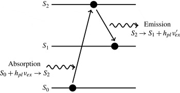
LIF is based on the principle that electrons of fluorescent molecules can be moved from a ground state ( $S_{0}$ ) to an electronically excited state ( $S_{2}$ ) by incident photons of energy $h_{pl}{\it\nu}_{ex}$ , as shown schematically in figure 1 (Crimaldi Reference Crimaldi2008). Here, $h_{pl}$ denotes Planck’s constant, and ${\it\nu}_{ex}$ is the frequency of incident light. The excited molecules relax to an intermediate state ( $S_{1}$ ) by emitting a photon excitation light of energy $h_{pl}{\it\nu}_{ex}^{\prime }$ due to collision of the excited molecules with surrounding molecules in the excited state. Owing to energy dissipation during the excited-state life time, the energy of an emitted photon is always lower than the excited energy of the photon (i.e. ${\it\nu}_{ex}^{\prime }<{\it\nu}_{ex}$ ).

Figure 1.

Absorption and emission of a photon by a fluorescent molecule due to the collision of a dye molecule with surrounding molecules.

The amount of absorbed excitation light by a given volume of fluid containing fluorescent molecules can be expressed by Beer–Lambert’s law,

(2.1) $$\begin{eqnarray}I_{A}=I_{0}-I_{0}\text{e}^{-{\it\epsilon}hc}=I_{0}(1-\text{e}^{-{\it\epsilon}hc}).\end{eqnarray}$$

Here, $I_{A}$ denotes the absorbed power, $I_{0}$ stands for the excitation power, ${\it\epsilon}$ is the molar extinction coefficient which depends on the wavelength of the incident light, $h$ represents the path length through the sample, and $c$ is the concentration of fluorophore species. Accordingly, the amount of emitted fluorescence energy ( $I_{f}$ ) is proportional to the absorbed energy ( $I_{A}$ ) and the quantum efficiency of the dye ( ${\it\phi}_{dye}$ ),

(2.2) $$\begin{eqnarray}I_{f}=I_{A}{\it\phi}_{dye}=I_{0}{\it\phi}_{dye}(1-\text{e}^{-{\it\epsilon}hc}).\end{eqnarray}$$

2.2. Applying LIF to a moving liquid sheet formed by jet impingement

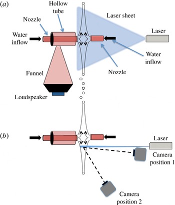
The schematic diagram of the experimental set-up is shown in figure 2, and is similar to that reported earlier (Mulmule, Tirumkudulu & Ramamurthi Reference Mulmule, Tirumkudulu and Ramamurthi2010). Two identical converging nozzles made up of borosilicate glass with an exit diameter of 1.62 mm and a length of 12 cm are used in the present experiments to obtain liquid sheets over a range of Weber numbers ( $We_{d}=300{-}1000$ ). A three-dimensional traverse is used to position the two nozzles so that the gap between the two nozzles is maintained at approximately 3 mm, and the horizontal axes of the two nozzles are adjusted with rotating stages so that they are accurately aligned. A gear pump is used to pump the liquid from a tank to the nozzles, and the flow through the nozzles is controlled with the help of rotameters. The gear pump delivers smooth and pulseless flow, and consequently does not introduce disturbances into the flow. Experiments were also performed by connecting the piping to a continuous supply of water from overhead tanks situated at a height of around 16 m with respect to the experimental set-up. The results were identical, and therefore most experiments were performed with the pump. Flow through the rotameters is calibrated with the help of a measuring cylinder and the measurement error in flow rate was less than 4 %. Two air vent valves are used to remove air bubbles so as to eliminate disturbances in the flow. The liquid sheet is formed by a head-on impingement of two opposing jets; ejected droplets from the periphery of the sheet are collected in a tray placed below the traverse, and the same is recirculated to the tank. The axial distance between the tip of each nozzle and the point of jet collision was carefully adjusted to obtain a smooth and steady liquid sheet.

Figure 2.

Schematic diagram of the experimental set-up. (a) Side view including the speaker arrangement for introducing disturbances at the impingement point. (b) Top view with the camera positions for measuring the thickness modulation (position 1) and centreline displacement (position 2).

The components necessary to carry out the liquid-sheet thickness measurements are the jet impingement set-up as described above, fluorescent dye, an incident laser light sheet and an optical system for the measurement of the fluorescent emission. We chose Rhodamine 6G fluorescent dye for the present work because its physical properties are ideal: absorption (530 nm) and emission (560 nm) spectra are completely separate, the dye is water-soluble and has high quantum efficiency and, furthermore, its excitation wavelength matches the available Argon-Ion laser light source. The fluorescent dye of known concentration is uniformly mixed in water to avoid the formation of any dye aggregates. A thin vertical laser sheet ( ${\sim}0.1~\text{mm}$ thickness) is generated by passing the laser beam through a cylindrical lens. The vertical laser sheet slices the liquid sheet in a direction perpendicular to the liquid sheet (figure 2). This results in the emission of fluorescent light along a vertical line formed by the intersection of the laser sheet and the liquid sheet. The laser sheet is passed slightly off-centre through the liquid sheet as the piping system and the nozzle arrangement prevent it from passing through the centre of the liquid sheet. The emission from the fluorescent region is captured with a light-sensitive high-speed CCD camera (Pike^® F032B model) for varying liquid flow rates. The camera is capable of achieving frame rates up to 1000 f.p.s. at a pixel resolution of $640\times 50~\text{pixels}$ . The measurement of the liquid-sheet thickness and the position of the centreline of the liquid sheet require two different camera positions. For the former, the camera is placed facing the liquid sheet almost parallel to the laser sheet (camera position 1, figure 2 b) so that the intensity variations due to thickness modulations can be observed clearly. The camera is placed at an acute angle to the liquid-sheet surface (camera position 2, figure 2 b) for the measurement of the liquid sheet’s centreline displacement.

For the conditions of the experiments presented here, the product of the molar extinction coefficient and dye concentration is in the range $c{\it\epsilon}=54$ – $62~\text{cm}^{-1}$ with the value of ${\it\epsilon}=116\,000~\text{M}^{-1}~\text{cm}^{-1}$ (Birge Reference Birge1987). As the thickness of the liquid sheet is very small $(h\ll 1/{\it\epsilon}c)$ , (2.2) can be simplified to obtain the fluorescence emission at any location on the sheet:

(2.3) $$\begin{eqnarray}I_{thin}\approx I_{0}{\it\phi}_{dye}{\it\epsilon}hc.\end{eqnarray}$$

The above expression shows that the fluorescence emission is proportional to the incident light intensity, dye characteristics of fluorophore and path length of the liquid film. Once the concentration of the fluorescent species and the solvent is fixed, the only unknown in (2.3) apart from the film thickness is the laser sheet intensity ( $I_{0}$ ) along its transmitted path through the liquid sheet. The incident laser sheet intensity varies spatially, which was determined by performing calibration experiments with optically thick films of known thickness $(h\gg 1/{\it\epsilon}c)$ , so that for the conditions of the experiments, (2.2) simplifies to

(2.4) $$\begin{eqnarray}I_{thick}\approx I_{0}{\it\phi}_{dye}.\end{eqnarray}$$

In our experiments, thick films were obtained by using a rectangular cuvette of known dimensions (height 20 cm, width 4 cm, thickness 1 cm) filled with the same fluorescent solution as that used for the liquid sheet experiment. The cuvette was placed in the path of the laser sheet at the same location as the liquid sheet. The fluorescence emission from the illuminated vertical section of the cuvette was recorded with all settings of the laser and the camera, such as the laser operating power, camera position, shutter speed and exposure time, kept identical to that for the liquid-sheet experiments. Once $I_{thick}$ is known, (2.3) and (2.4) together give the thickness of the liquid sheet:

(2.5) $$\begin{eqnarray}h=\frac{I_{thin}}{I_{thick}{\it\epsilon}c}.\end{eqnarray}$$

The fluorescent intensities are obtained by post-processing the captured images in terms of grey levels along the illuminated sections (using ImageJ^® and Matlab^® software).

2.3. Liquid-sheet experiments with acoustic forcing close to the jet impingement location

Acoustic disturbances were introduced close to the jet impingement location resulting in an undulating liquid sheet. This was achieved with a high-sound-intensity speaker (P Audio^® C12-500 MB, 50 Hz–2 kHz, programming power of 500 W and sensitivity of 96 dB) connected to a QSC^® GX5 (500 W @ $8~{\rm\Omega}$ ) amplifier, which in turn was connected to an Agilent^® 33220A signal generator. The latter was tuned to generate signals of varying frequencies and amplitudes. The mouth of the speaker was covered by the diverging end of a conical funnel while the converging end was connected to a hollow tube concentric with one of the water nozzles (figure 2 a). The quality of the acoustic signals close to the impingement location was checked with the help of a B&K^® 2250L sound level meter for different frequencies and sound pressure levels (SPLs). In all cases, the frequency of the dominant peak was identical to that generated by the signal generator. Peaks were also observed at higher harmonics but their intensity was lower by at least 30 dB. As soon as the acoustics are switched on, waves appear close to the impingement location and propagate outwards along the radial direction. It was also ensured that the sound level was uniform around the mouth of the nozzle. This was confirmed by measuring the SPL at different locations around the nozzle.

We also checked whether acoustic forcing causes any significant variation in the diameter of the liquid jet. The jet was imaged at various frequencies and amplitudes, and it was found that there was no perceptible variation in the jet diameter, at least within the camera’s resolution ( $1~\text{pixel}=8~{\rm\mu}\text{m}$ ), which is less than 1 % of the jet diameter. We also determined whether external acoustic forcing leads to flow rate variations. Polyamide particles were dispersed in water and their motion was imaged inside the nozzle in the presence of acoustic forcing. A laser sheet aligned along the axis of the nozzle and intersecting it along its vertical diameter revealed the motion of the particles via a camera placed transverse to the plane of the sheet. The captured images are processed to track the position of particles with time for each applied frequency, and the velocity of the particles for each radial position was determined as a function of time. There was no perceptible periodic motion of the particles with acoustic forcing within the resolution of the applied technique, with the velocity being the same irrespective of the forcing frequency. These results demonstrate that there is no variation in jet diameter, nor is there any change in the velocity of the fluid in the presence of acoustic forcing. Based on the above tests and the visualization of the displacement of the sheet under fluorescence (to be described later), it is concluded that sinuous disturbances originate at the impingement point and are convected radially outwards.

Finally, the sheet displacement at any location (along the fluorescent line) is obtained by subtracting the position of the fluorescent line in the presence of acoustics with that in its absence. As figure 2 shows, the camera in position 2 is used to determine the displacement of the sheet centreline. Given that the line of sight (represented by the dashed line) is at an angle of about $10^{\circ }$ to the plane of the liquid sheet, the measured displacement will be somewhat less (by $\cos (10^{\circ })\sim 0.984$ ) than the true value. However, the normalized displacement of the sheet centreline obtained by scaling the measured displacement with that measured at the lowest radial location, will be the same irrespective of this angle. We also note that the largest displacements lead to relatively small slopes ${\sim}0.2{-}0.3$ (angle ${\sim}10^{\circ }{-}15^{\circ }$ ). For very large slopes, we expect sections of the fluorescent line to be blocked by parts of the deformed sheet present in the light path between the fluorescent line and the camera. However, this did not happen in any of the experiments, confirming that the deformations were small.

3.1. Thickness distribution of a smooth liquid sheet in the absence of forcing

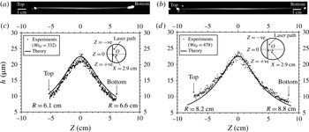
Figures 3(a) and 3(b) present the emissions from the fluorescent section of liquid sheet for $We_{d}=332$ and 478, respectively, which was off-centre by 2.9 cm from the impingement point. The emission images have been rotated by $90^{\circ }$ , with the direction of gravity being from left to right. The corresponding extracted thickness distribution along the vertical fluorescent line is given in figures 3(c) and 3(d), respectively. The solid line in the plots represents the theoretical thickness distribution (1.1). The measurements closely follow the theoretical line for the entire thickness range. The scatter in the experimental data was quantified by calculating the standard deviation about a moving average of the experimental data points. For all cases, the standard deviation was less than $0.5~{\rm\mu}\text{m}$ (which sets the resolution of the technique). An important point to note from figure 3(c,d) is that the measured thickness profile is nearly identical for the two cases, thereby confirming that the thickness profile is independent of $We_{d}$ . The maximum thickness along the vertical line for both cases is found to be $h_{max}=23\pm 0.5~{\rm\mu}\text{m}$ , which closely matches the theoretical value $h_{max}=22.5~{\rm\mu}\text{m}$ .

Figure 3.

(a,b) Emission from the fluorescent section of the liquid sheet for (a)  $We_{d}=332$ and (b)  $We_{d}=478$ . The emission images have been rotated by $90^{\circ }$ with the direction of gravity being from left to right. (c,d) The corresponding extracted thickness distributions. The solid line represents the theoretical thickness distribution (1.1). The insets in (c,d) include a schematic of the circular sheet along with the position of the intersecting vertical laser sheet. The bright rim region at the sheet edge seen in (a,b) has been omitted in the plot.

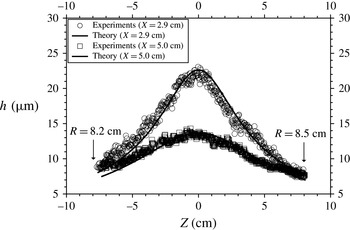
Figure 4 shows the thickness distribution of a smooth liquid sheet ( $We_{d}=540$ ) at two different vertical sections off-centre by 2.9 and 5.0 cm from the impingement point. Since the vertical sections are different for the two cases, the profiles are also different. For the profile that is 2.9 cm away from the impingement point, $h_{max}=23\pm 0.5~{\rm\mu}\text{m}$ , and that for 5.0 cm, $h_{max}=13.8\pm 0.5~{\rm\mu}\text{m}$ , both of which agree rather well with the theoretical maximum-thickness values of 22.5 and $13~{\rm\mu}\text{m}$ , respectively. Close inspection of the measured profiles in all cases (including figure 3 c,d) shows that the sheet thickness in the upper regions of the sheet is slightly larger than that in the lower region of the sheet. This small difference is attributed to the effect of gravity, which slows the liquid as it flows upwards, leading to a marginally larger-than-predicted thickness in the upper regions and vice versa for the lower regions of the sheet.

Figure 4.

Thickness distribution of a liquid sheet for $We_{d}=540$ at two different vertical sections that are off-centre by 2.9 cm, and 5.0 cm from the jet impingement point. The solid line represents the theoretical prediction (1.1).

These results suggest that the LIF technique can be successfully employed to measure the thickness distribution of thin moving liquid sheets. Next, the technique is applied to undulating liquid sheets to determine both the thickness modulation and the position of the centreline.

3.2. Thickness distribution of a liquid sheet with acoustic forcing

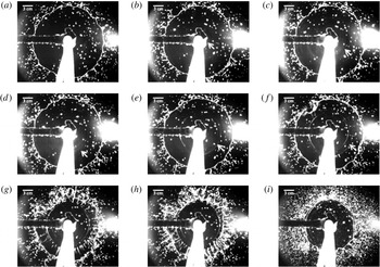
Before discussing the results of the LIF technique, it is instructive to visualize the undulating liquid sheet under normal light conditions. Figure 5(a–i) show the response of the liquid sheet at $We_{d}=540$ subjected to forcing at a frequency of 90 Hz and an SPL of 85 dB at the impingement point. Figure 5(a) shows the smooth liquid sheet just before the acoustics was introduced. After switching on the acoustics, surface ripples appear first near the impingement location, and they travel outwards along the radial direction. The presence of ripples is clear in images from $t=13/500~\text{s}$ onwards, although close inspection reveals their presence near the impingement point at $t=3/500~\text{s}$ . When the surface ripples reach a distance of about 4 cm from the rim, radial streaks originate and expand towards the edge of the sheet (figure 5 g,h), leading to a catastrophic break-up of the sheet edge. The liquid sheet suddenly shrinks in size by ejecting tiny jets of water from the circumference of the sheet, as shown in figure 5(g,h). The liquid sheet finally reaches a stable but smaller size and continues to flap in response to the acoustics (figure 5 i). These images appear similar to those of Mulmule et al. (Reference Mulmule, Tirumkudulu and Ramamurthi2010), where the entire liquid sheet is subjected to external acoustic waves, and those of Bremond et al. (Reference Bremond, Clanet and Villermaux2007), where undulations were produced by a head-on impingement of a single laminar jet on a vibrating impactor.

Figure 5.

Time evolution of the deformation of a smooth liquid sheet ( $We_{d}=540$ ) excited by a disturbance introduced at the impingement point with a forcing frequency of 90 Hz and an SPL of 85 dB. The white scale bar at the top left corner of each image corresponds to 3.0 cm. The white arrow follows a sinuous wave as it moves out radially. The time elapsed after turning on the acoustics for each subfigure is as follows: (a)  $t=0~\text{s}$ ; (b)  $t=3/500~\text{s}$ ; (c) $t=6/500~\text{s}$ ; (d) $t=9/500~\text{s}$ ; (e) $t=13/500~\text{s}$ ; (f) $t=15/500~\text{s}$ ; (g)  $t=17/500~\text{s}$ ; (h) $t=18/500~\text{s}$ ; (i) fully developed sheet.

As the above studies have demonstrated, the ripples correspond to sinuous waves that travel radially outwards from the impingement point. In the present case, the phase speed of the sinuous wave is smaller than the liquid speed, and this is confirmed by noting that the ripples (in figure 5) take about 0.034 s to travel about 7 cm radially outwards compared to 0.014 s (calculated from the known jet speed) for a liquid element for the same distance. The radius of the undisturbed sheet is about 10 cm (figure 5 a). Furthermore, the time period of a single acoustic cycle in figure 5 is 0.011 s, indicating that every fluid element sees one full acoustic cycle before reaching the edge.

We used the LIF technique to capture the thickness modulations and thus the varicose mode of the undulating liquid sheet in the presence of acoustic forcing. Before performing the experiments on the liquid sheet, we tested the applicability of the technique on an undulating soap film forced by acoustics. The measured relative thickness distribution agreed well with those obtained via the interference technique (Boudaoud, Couder & Amar Reference Boudaoud, Couder and Amar1999) in terms of the location of the minima and maxima in the thickness distribution, thereby establishing the applicability of the LIF technique for measuring the thickness of undulating films.

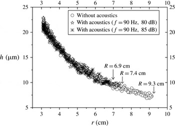
Next, the thickness modulation was obtained for a liquid sheet at $We_{d}=540$ , subjected to a frequency of 90 Hz and forced at two different SPLs, namely, 80 and 85 dB. Capturing the initial transient in the thickness modulation, when the outer sections of the sheet break, was difficult because of the formation of radial streaks on the sheet. The latter appear as bright spots in the captured fluorescence images and prevent reliable measurement of the thickness during this time interval. Therefore, in all cases, measurements were made after the sheet had reached a stable size following the initial transient. The film thickness profile is presented in figure 6 for the two cases along with that measured in the absence of acoustics. As expected, the sheet radius $R$ reduces with an increase in the SPL. Clearly, within the resolution of the technique (standard deviation of $\pm 0.5~{\rm\mu}\text{m}$ ), there are no perceptible thickness modulations in the liquid sheet at the two SPLs; they match with the thickness obtained in the absence of acoustics, indicating that thickness modulations, if any, are below the resolution of the experimental technique. Therefore, in what follows, the focus will be on the dynamics of the sinuous wave.

Figure 6.

Thickness distribution of a fully developed liquid sheet ( $We_{d}=540$ ) when it is excited at 90 Hz at two different SPLs of 80 and 85 dB. Note that the thickness is plotted as a function of the radial distance from the impingement point. The distance between the fluorescent vertical section on the liquid sheet and the impingement location is 3.0 cm. The radial extent of the sheet ( $R$ ) is included for each case.

3.3. Growth rates and phase velocities of the sinuous wave

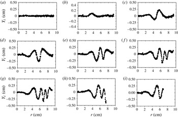
The centreline position of the liquid sheet was obtained by an analysis of images that were taken by the camera located at position 2 (figure 2 b). The centreline position corresponds to the location of the maximum-intensity pixel along the length of the vertical fluorescent section of the liquid sheet. Experiments were performed in the frequency range of 60–250 Hz and at different SPLs. Figure 7 presents the centreline position of the liquid sheet as a function of the radial coordinate at different time steps for $We_{d}=540$ and for an acoustic forcing at 80 Hz, 80 dB. Here, $Y_{i}$ is the deviation of the sheet’s centreline position from its base state (i.e. in the absence of acoustics), and the time data in each subfigure correspond to the time elapsed after switching on the acoustics. The subfigure also includes the radius of the liquid sheet in each frame. The images for this data set were taken at a frame rate of 442 f.p.s.

Figure 7.

Time evolution of the sheet’s centreline position for $We_{d}=540$ when excited with a forcing frequency of 80 Hz and an SPL of 80 dB. The images are captured at a frame rate of 442 f.p.s. (a) $t=0~\text{s};R=9.2~\text{cm}$ , (b) $t=3/442~\text{s};R=9.2~\text{cm}$ , (c)  $t=7/442~\text{s};R=9.2~\text{cm}$ , (d) $t=10/442~\text{s};R=9.2~\text{cm}$ , (e) $t=14/442~\text{s};R=9.2~\text{cm}$ , (f) $t=19/442~\text{s};R=9.2~\text{cm}$ , (g) $t=21/442~\text{s};R=9.1~\text{cm}$ , (h) $t=24/442~\text{s};R=7.6~\text{cm}$ , (i) $t=27/442~\text{s};R=6.8~\text{cm}$ . The radial position of the last point on the right gives the radial extent $(R)$ of the sheet.

As soon as the forcing is turned on, the central section of the liquid sheet is displaced first, which subsequently generates a sinuous wave that travels radially outwards. The amplitude of the wave increases initially as it propagates some distance, and thereafter starts to decrease close to the rim. The outer regions of the sheet break at around $t=24/442~\text{s}$ when the sinuous wave nearly reaches the rim of the sheet. Note that this occurs after more than four time cycles of forcing, confirming that regions close to the impingement point are displaced first. The sheet radius reduces to a stable value of 6.8 cm at $t=27/442~\text{s}$ , though the sheet continues to respond to forcing.

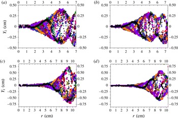
The time evolution of the sinuous wave yields the wave envelope that consists of data points corresponding to the maximum displacement of the sinuous wave along the length of the sheet. The envelope was obtained by overlapping the wave forms of at least 30 consecutive time points (more than four time cycles for most frequencies tested). Figure 8 presents four such plots, two each for $We_{d}=540$ and 990. While the former corresponds to the smooth regime, the latter falls within the transition regime. Comparison of the overall profile of the envelopes indicates no qualitative difference between the profiles for the two regimes. In all four cases, the sheet-centreline displacement increases with radial location close to the impingement point, suggesting that the liquid sheet is spatially unstable to perturbations introduced close to the impingement point. The envelope exhibits a peak that occurs at a smaller radial distance for the lower $We_{d}$ compared to that observed for $We_{d}=990$ . The envelope for the lower $We_{d}$ appears to rise towards a second peak before reaching the edge of the sheet, while the sheet breaks before the appearance of such a feature at the higher $We_{d}$ .

Figure 8.

Experimental envelopes of a liquid sheet of $We_{d}=540$ and 990 forced at frequencies of 80 and 90 Hz. (a) $We_{d}=540$ , 80 Hz, 85 dB; (b) $We_{d}=540$ , 90 Hz, 85 dB; (c) $We_{d}=990$ , 80 Hz, 70 dB; (d) $We_{d}=990$ , 90 Hz, 70 dB. In all four cases, the sheet has reached a steady size after an initial transient.

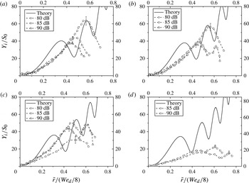
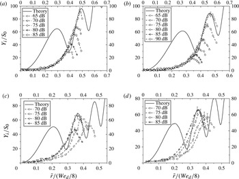
Given the similarity of the envelopes for the smooth and the transition regimes, in figures 9 and 10, we compare the measured envelope with the predictions of the recent theory of Tirumkudulu & Paramati (Reference Tirumkudulu and Paramati2013), which neglects the presence of the gas phase and is strictly applicable only in the smooth regime. The radial coordinate is rendered dimensionless with the diameter of the jet, $\tilde{r}\equiv r/d$ , so that $\tilde{r}/(We_{d}/8)=1$ corresponds to the edge of the circular sheet in the absence of acoustics (1.2). The non-dimensional displacements collapse for various SPLs in both cases, indicating a linear response. However, larger sheets are observed for lower SPLs. The breaking of the liquid sheet indicates the presence of thickness modulations. Bremond et al. (Reference Bremond, Clanet and Villermaux2007) suggest that a flapping sheet should be unstable to modulations induced by Rayleigh–Taylor instability for large transverse oscillations of the liquid sheet. In our experiments, large initial amplitudes (due to high dB) for a fixed frequency would lead to large transverse acceleration downstream of the impingement point, thereby breaking the sheet at a lower radial distance. Such effects may be explained by accounting for the aforementioned instability, but are beyond the scope of the current investigations.

Figure 9.

Sinuous wave envelope for $We_{d}=540$ at varying forcing frequencies and SPLs. (a) 80 Hz; (b) 90 Hz; (c) 100 Hz; (d) 110 Hz.

Figure 10.

Sinuous wave envelope for $We_{d}=990$ at varying forcing frequencies and SPLs. (a) 80 Hz; (b) 90 Hz; (c) 140 Hz; (d) 150 Hz.

The experimental error in the measurement of the centreline position due to the finite size of the camera pixel is represented by an error bar, and is included only for the data point representing the maximum displacement. Note that the error bars for the rest of the data points for a given set have not been shown but are identical to those for the maximum displacement. The evolution of sinuous disturbance from theory is obtained by plotting the complex roots ( $S_{r}(\bar{r})\cos (\bar{{\it\omega}}\bar{t})-S_{i}(\bar{r})\sin (\bar{{\it\omega}}\bar{t})$ ) of (1.8) at different time steps, where $S_{r}$ and $S_{i}$ are the real and imaginary parts, respectively, of the disturbance. The theoretical envelope was obtained by overlapping the above solution for many time steps for the experimental frequencies. The initial dimensionless displacement was obtained from the measured value closest to the impingement point. Figure 9 presents the results for the smooth regime ( $We_{d}=540$ ) for four different frequencies. At the lowest two frequencies, the predicted envelope exhibits a spatial growth rate similar to that observed, except for the presence of an early peak (or antinode) in the theoretical profile that is absent in the experiments. The magnitude of the envelopes predicted by theory matches remarkably well for distances far from the point of impingement (i.e. after the first peak). As the frequency increases, the theory predicts an increasing number of peaks in the envelope over the same spatial domain. A similar observation is made in experiments, where a second peak is observed at 100 Hz (85 and 90 dB). At the highest frequency tested (110 Hz), the measured envelope is below that predicted by theory. It was observed that as the frequency was increased, a larger SPL was required to observe a perceptible response. Thus a weak response was observed for 100 Hz at 80 dB, while there was no measurable response for 110 Hz at the same SPL. These observations can be explained by balancing the periodic forcing across a section of the liquid sheet close to the point of impingement with mass times the acceleration imparted to that section,

(3.1) $$\begin{eqnarray}P_{m}\cos ({\it\omega}t)\sim h{\it\rho}_{l}\frac{\text{d}^{2}z}{\text{d}t^{2}},\end{eqnarray}$$

where $P_{m}$ is the magnitude of the pressure difference across the section of the sheet of thickness $h$ , and $z$ denotes the displacement of the section of the sheet. Integrating the above relation in time gives

(3.2) $$\begin{eqnarray}z\sim \frac{P_{m}\cos ({\it\omega}t)}{h{\it\rho}_{l}{\it\omega}^{2}},\end{eqnarray}$$

suggesting that the displacement imparted to the impingement point will decrease inversely with the square of the forcing frequency. For small displacements, viscous dissipation may damp out the disturbances, leading to non-overlapping growth curves (figure 9 c).

Next, the predictions are compared to the envelopes obtained for the higher $We_{d}$ (figure 10) which lies in the transition regime. As before, the measured envelopes collapse for the various SPLs for the two lower frequencies. In contrast to the lower $We_{d}$ , only a single peak is observed at all frequencies and SPLs. The sheet was far more sensitive to perturbations, since an SPL as low as 65 dB was able to elicit a measurable response. Again, the first peak predicted by theory is missing in the experiments, although the observed trend of the sinuous disturbance is similar to that predicted and the height of the predicted envelope matches the measurements far from the impingement point. The sheet was unstable for a range of SPLs and for the frequencies tested. At the two higher frequencies of 140 and 150 Hz, the envelopes are similar only at the highest SPLs. These results clearly show that even at a Weber number as high as 990, the amplitude of the envelope predicted by the model is of the same magnitude as that observed in experiments. The mismatch between prediction and measurements for both high and low $We_{d}$ occurs at short distances from the impingement point. Specifically, the first peak in the envelope is not observed in the experiments. While the cause of this discrepancy is not clear, it could be attributed to one of the several approximations made in the model. First, the model assumes that the sheet thickness is small compared to the radial distance; hence it is not applicable to regions close to the impingement point. As Crapper & Dombrowski (Reference Crapper and Dombrowski1984) note, the rapid rate of thinning in these regions would indeed influence the growth rate, and it is expected to be different from that predicted by our asymptotic solution. It is also possible that the presence of the surrounding gas phase in the experiments influences the initial growth rate due to the added mass effect, since for high initial growth rates the sheet will have to move the surrounding gas very rapidly, thereby increasing the inertia of the liquid sheet. Finally, the observed growth rates could also be lower due to the dampening effect of liquid and/or gas viscosity. Despite the approximations of the model, it should be noted that it is free of adjustable constants, and the envelope (non-dimensional) is a function of the Weber number and the forcing frequency alone.

At this stage, it is instructive to determine the stability of the liquid sheet in the presence of the gas phase from the analysis of Squire (Reference Squire1953), which accounts for the aerodynamic interactions in a constant-thickness sheet, and compare it with our theory. The dispersion equation of Squire obtained for a moving liquid sheet of constant thickness is given by

(3.3) $$\begin{eqnarray}{\it\rho}_{l}\left(\frac{{\it\omega}}{k}-U\right)^{2}\tanh \left(\frac{kh}{2}\right)+{\it\rho}_{g}\left(\frac{{\it\omega}}{k}\right)^{2}={\it\sigma}k,\end{eqnarray}$$

where $k$ is the wavenumber and the disturbance is assumed to be of the form $\exp \;(\text{i}(kx-{\it\omega}t))$ , where $x$ is the spatial coordinate. In the limit of large wavelengths such that $kh\ll 1$ , the dimensionless form of the dispersion relation reduces to

(3.4) $$\begin{eqnarray}\tilde{k}^{3}\left[\frac{1}{2}-\frac{4\tilde{r}}{We_{d}}\right]-\tilde{k}^{2}\tilde{{\it\omega}}+\tilde{k}\left[\frac{\tilde{{\it\omega}}^{2}}{2}\right]+4\tilde{r}{\it\delta}\tilde{{\it\omega}}^{2}=0,\end{eqnarray}$$

where ${\it\delta}={\it\rho}_{g}/{\it\rho}_{l}$ , $\tilde{k}=kd$ , $\tilde{r}=r/d$ , and $\tilde{{\it\omega}}={\it\omega}d/U$ and the film thickness is a function of the radial coordinate ( $h=d^{2}/4r$ ). It can be confirmed that in the absence of the gas phase $({\it\delta}=0)$ , the above equations predict temporal (neutral) stability irrespective of the value of the film thickness. A similar, ‘locally parallel’ ad hoc assumption, applied to the stability (1.5) for sinuous disturbances on a radially expanding sheet with disturbance of the form $\exp \;(\text{i}(kr-{\it\omega}t))$ , gives an approximate dispersion relation that accounts for the effects of sheet thinning alone,

(3.5) $$\begin{eqnarray}\tilde{k}^{2}\left[\frac{1}{2}-\frac{4\tilde{r}}{We_{d}}\right]+\tilde{k}\left[-\tilde{{\it\omega}}+\frac{\text{i}}{\tilde{r}}\left(\frac{1}{2}+\frac{4\tilde{r}}{We_{d}}\right)\right]+\left[\frac{\tilde{{\it\omega}}^{2}}{2}-\text{i}\frac{\tilde{{\it\omega}}}{2\tilde{r}}\right]=0,\end{eqnarray}$$

where $\tilde{r}=r/d$ . Close inspection of the above dispersion relation shows that it reduces to (3.4) for the case ${\it\delta}=0$ , when $1/\tilde{r}\rightarrow 0$ ( $4\tilde{r}/We_{d}$ is bounded).

For the experiments discussed here, wherein the forcing frequency is held fixed while the spatial growth of the sinuous wave is sought, we next investigate the spatial stability using the above two equations (3.4) and (3.5) to evaluate the relative importance of aerodynamic interactions and thinning on the stability of radially expanding liquid sheets. This involves treating $\tilde{k}$ as complex for given real values of $\tilde{{\it\omega}}$ and determining the wavenumber with the largest (in magnitude) negative imaginary part. Furthermore, it is confirmed that the solution satisfies the causality condition in that the corresponding group velocity is positive for $\tilde{x},\tilde{r}>0$ .

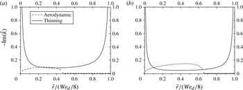
Figure 11 plots the most unstable spatial growth rate as a function of the radial distance obtained by solving (3.4), which accounts for aerodynamic interactions, and (3.5), which includes the effect of sheet thinning. For regions close to the impingement point and the rim, the spatial growth rates diverge due to the thinning effect. This is because of the imaginary terms in the coefficient of $\tilde{k}$ . In comparison, the spatial growth rate due to the aerodynamic interactions increases from zero, reaching a maximum at some radial location and subsequently decreasing to zero within the extent of the radial sheet. For the low $We_{d}\;(=540)$ , the thinning effects dominate everywhere except for a small region where the spatial growth rates due to the aerodynamic effects are marginally greater. For the higher $We_{d}$ , the aerodynamic effects dominate between radial positions (non-dimensional) of 0.1 and 0.65 while the thinning effects are important outside this region. These results suggest that while aerodynamic interactions will dominate at high $We_{d}$ over the majority of the sheet, there will be regions close to the impingement point and near the sheet edge where thinning effects will dominate.

Figure 11.

The most unstable spatial growth rate for the dispersion relation obtained from our theory (thinning) and that obtained from Squire’s theory (aerodynamic) as a function of the radial location for $We_{d}=540$ and 990 at 80 Hz. (a) $We_{d}=540$ , $\tilde{{\it\omega}}=0.16$ (80 Hz); (b) $We_{d}=990$ , $\tilde{{\it\omega}}=0.12$ (80 Hz).

It is possible to determine the range of frequencies over which the most unstable spatial mode due to aerodynamic interactions is higher than that due to thinning for some radial location, so that for frequencies outside this range, the thinning effects dominate everywhere on the sheet (i.e. the dashed line in figure 11 is always below the solid line). Figure 12(a) presents the regime map obtained from such a calculation, which delineates regions where the thinning effects dominate from regions where both effects become important. The regime map applies for liquid sheets produced by the impingement of two jets. For $We_{d}<509$ and irrespective of the forcing frequency, the spatial growth rates due to the thinning effect are greater than those due to aerodynamic interactions at all radial locations of the thinning sheet. For $We_{d}>509$ and over a frequency range, the spatial growth rates due to aerodynamic effects are higher than those due to the thinning effect over a section of the sheet, though the predicted rates due to thinning diverge close to the impingement point and sheet edge, and always dominate at these locations. Thus $We_{d}=509$ is the critical Weber number above which the aerodynamic effects will become important over some section of the sheet and for a certain range of forcing frequencies. The plot includes our experimental points for both $We_{d}=540$ and 990 and at all forcing frequencies tested in this study. Even though the points for $We_{d}=540$ suggest an influence of both thinning and aerodynamic interactions, the plot of spatial growth rate versus radial position indicates that aerodynamic effects are marginally more important over a small region of the sheet while the thinning effects dominate everywhere else. However, at higher $We_{d}$ , larger regions of the sheet are more susceptible to instabilities due to aerodynamic interactions than due to thinning effects. Yet, the nature of agreement between the predicted envelopes from our theory and those measured for both high and low $We_{d}$ appears similar (figures 9 and 10). Indeed, Dombrowski and co-workers (Clark, Dombrowski & Pyott Reference Clark, Dombrowski and Pyott1975) measured the spatial growth of sinuous waves on radially thinning liquid sheets produced by vibrating fan spray nozzles in the flapping regime, and found that Squire’s analysis overpredicts the spatial growth rates for sinuous disturbances; they attributed the difference to the formation of vortices from wave crests, which dampen the wave growth.

Figure 12.

Regime map where the line (with $\circ$ ) delineates regions in the $\tilde{{\it\omega}}{-}We_{d}$ space where the thinning effects dominate and regions where effects due to both aerodynamic interactions and thinning are important. (a) This plot corresponds to the case of the circular sheet produced by head-on impingement of two jets, where $h=d^{2}/4r$ . The points ( $\times ,+$ ) correspond to our experiments, $We_{d}=540$ and 990. (b) This plot corresponds to the case of the circular sheet produced by a single jet impinging head-on onto an impactor, where $h=d^{2}/8r$ . The points ( $\times ,+$ ) correspond to experiments of Bremond et al. (Reference Bremond, Clanet and Villermaux2007) for $We_{d}=$ 850 and 990.

More recently, Bremond et al. (Reference Bremond, Clanet and Villermaux2007) studied the dynamics of sinuous disturbances on a circular liquid sheet formed by a single laminar jet impinging on a vibrating impactor, and studied the growing sinuous wave in the transition/flapping regime. They derive the spatial growth rate from Squire’s analysis (their (3.23)), based on which, they further derive an expression for a cut-off forcing frequency beyond which the sheet is unstable for radial distances less than the radius of the impact cylinder and thus considered stable. They find that the sinuous waves grow even for frequencies beyond the cut-off value and attribute it to the naturally most-amplified mode. The predicted growth rate from Squire’s theory was found to be about twice that observed, and so they multiply the predicted growth rate by a factor of one half to match the measurements. However, in light of our findings, the sheet should be unstable even beyond the cut-off frequency, due to thinning effects where the spatial growth corresponding to the forcing frequency is determined from (1.8). For the case of a single jet impinging on an impactor, the film thickness is given by $h=d^{2}/8r$ , and the corresponding dispersion relation that accounts for aerodynamic interactions is given by

(3.6) $$\begin{eqnarray}\tilde{k}^{3}\left[\frac{1}{2}-\frac{8\tilde{r}}{We_{d}}\right]-\tilde{k}^{2}\tilde{{\it\omega}}+\tilde{k}\left[\frac{\tilde{{\it\omega}}^{2}}{2}\right]+8\tilde{r}{\it\delta}\tilde{{\it\omega}}^{2}=0,\end{eqnarray}$$

while the dispersion relation due to thinning alone is

(3.7) $$\begin{eqnarray}\tilde{k}^{2}\left[\frac{1}{2}-\frac{8\tilde{r}}{We_{d}}\right]+\tilde{k}\left[-\tilde{{\it\omega}}+\frac{\text{i}}{\tilde{r}}\left(\frac{1}{2}+\frac{8\tilde{r}}{We_{d}}\right)\right]+\left[\frac{\tilde{{\it\omega}}^{2}}{2}-\text{i}\frac{\tilde{{\it\omega}}}{2\tilde{r}}\right]=0.\end{eqnarray}$$

Note that (3.6) is identical to (3.23) of Bremond et al. (Reference Bremond, Clanet and Villermaux2007).

Figure 12(b) presents the regime map for liquid sheets produced by impingement of a single jet against an impactor and applies to the experiments of Bremond et al. (Reference Bremond, Clanet and Villermaux2007). In this case, the thinning effects dominate for $We_{d}<721$ irrespective of the forcing frequency. Note that the critical value of $We_{d}=721$ is $\sqrt{2}$ times that for the two-jet case and is a consequence of the different thickness-dependence on the radial distance. The plot also includes points for their experiments at $We_{d}=850$ (140 to 260 Hz) and $We_{d}=990$ (100 Hz). 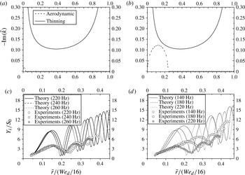All frequencies for the lower $We_{d}$ lie in the region where thinning dominates the spatial growth at all radial locations, and this is confirmed by plotting the most unstable spatial mode as a function of the radial distance for forcing frequencies of 240 Hz (figure 13 a) and 140 Hz (figure 13 b). While the spatial growth rates for thinning do not change much in this frequency range, those obtained from Squire’s dispersion relation reduce in magnitude and radial extent with increasing frequency. At the highest frequency (260 Hz), the magnitude and radial extent of spatial modes from Squire’s dispersion equation are insignificant compared to that obtained from our theory.

Figure 13.

(a,b) The most unstable spatial growth rate for the dispersion relation obtained from our theory (thinning) and that obtained from Squire (aerodynamic) as a function of the radial location for $We_{d}=850$ , (a) 240 Hz, and (b) 140 Hz. (c,d) The measured sinuous wave envelope for $We_{d}=850$ along with that predicted by (1.8) for (c) 220, 240 and 260 Hz, and (d) 140, 180, and 220 Hz. These conditions correspond to the experiments of Bremond et al. (Reference Bremond, Clanet and Villermaux2007). (a)  $\tilde{{\it\omega}}=0.95$ (240 Hz); (b)  $\tilde{{\it\omega}}=0.55$ (140 Hz); (c)  $\tilde{{\it\omega}}=0.55$ (140 Hz)–0.87 (220 Hz); (d)  $\tilde{{\it\omega}}=0.87$ (140 Hz)–1.02 (260 Hz).

Figures 13(c) and 13(d) plot, respectively, the corresponding measured envelopes of Bremond et al. (Reference Bremond, Clanet and Villermaux2007) for the reported range of forcing frequencies for $We_{d}=850$ . Based on Squire’s analysis, Bremond et al. (Reference Bremond, Clanet and Villermaux2007) predicted the sheet to be spatially stable for distances larger than the impactor’s radius for frequencies larger than a cut-off frequency, which was determined as 220 Hz for $We_{d}=850$ . This is evident from figure 13(a) for 240 Hz, where the spatial growth due to aerodynamic interactions is confined to a small region close to the origin. Frequencies larger than the cut-off value were considered to be in the stable forcing regime, while those below the value were supposed to be in the unstable forcing regime. Figures 13(c) and 13(d) also include the envelopes predicted by our theory. Here, the prediction of the sinuous wave envelope for the single-jet case is obtained by replacing the thickness profile for the two-jet case in (1.8) with that for a single jet, $h=d^{2}/8r$ . While the differences between the amplitudes of the nodes and antinodes of the predicted envelopes are larger than those observed in the experiments and the locations of the nodes and antinodes appear to be somewhat shifted, the overall growth is close to the observations. Specifically, the predicted positions of the nodes (and antinodes) grow spatially at rates similar to those observed. Not only is the measured distance between the first and second node (or antinode) for each frequency close to the predicted value, the shift in the location of the nodes (and antinodes) to lower radial location with frequency is also captured correctly by our model. Finally, the predicted first antinodes for the three frequencies corresponding to the stable forcing regime (figure 13 c) are very close together, while the distance is much larger for the lower frequencies (figure 13 d) which belong to the unstable forcing regime. The proximity of the antinodes in the stable forcing regime was used as evidence to support their assumption that the naturally most-amplified mode will be dominant, irrespective of the forcing frequency in the stable forcing regime. These features of the wave growth emerge naturally from our analysis which accounts for thinning of the sheet, suggesting that thinning effects play a dominant role here and are responsible for growth at all frequencies under these conditions.

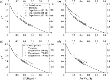
While the above discussion has focused on the growth of disturbances, it is also important to compare the measured phase velocity of the disturbance with that predicted by the two theories. The phase velocity, in our experiments, was measured by tracking the position of a particular crest of the growing sinuous wave in successive frames. Theoretically, the dimensionless phase speed for the fastest growing spatial mode is given by

(3.8) $$\begin{eqnarray}\tilde{v}_{p}=\frac{\tilde{{\it\omega}}}{\text{Re}[\tilde{k}]},\end{eqnarray}$$

where $\text{Re}[\tilde{k}]$ corresponds to the real part of the fastest growing spatial mode obtained from (3.4) and (3.5). Figure 14 compares the measured phase velocities for the two $We_{d}$ and for the two frequencies from our experiments with those obtained from both (3.4) and (3.5). Recall that the spatial growth due to aerodynamic interactions spans only part of the sheet, which is reflected in the prediction for the corresponding phase speed for only that section of the sheet. The measured phase speeds of the spatially growing wave match remarkably well with the predictions that account for the thinning effect, while those due to the aerodynamic interactions are higher than the observed values. While these results are consistent with the trend observed for the spatial growth predicted by (3.5) for the lower $We_{d}$ , the agreement for the case of higher $We_{d}$ where aerodynamic interactions dominate over the measured radial positions is surprising. The latter results seem to suggest that even when aerodynamic interactions are dominant, the phase speed of the growing waves is governed by the thinning of the liquid sheet. A combined theory that accounts for both effects may help resolve this discrepancy observed at high $We_{d}$ .

Figure 14.

Measured sinuous-wave phase speed for $We_{d}=540$ and 990 at varying forcing frequencies and SPLs along with predictions from (3.4) (aerodynamic) and (3.5) (thinning). (a) $We_{d}=540$ , $\tilde{{\it\omega}}=0.16$ (80 Hz); (b) $We_{d}=540$ , $\tilde{{\it\omega}}=0.19$ (90 Hz); (c)  $We_{d}=990$ , $\tilde{{\it\omega}}=0.12$ (80 Hz); (d) $We_{d}=990$ , $\tilde{{\it\omega}}=0.14$ (90 Hz).