

1. Introduction
While the US dollar remains the dominant global currency, its status is increasingly at risk due to policy uncertainty—particularly surrounding the Mar-a-Lago Accord—, rising national debt, and mounting pressure on the Federal Reserve’s independence. These risks are compounded by increasing geopolitical bloc formation and threaten to undermine the dollar’s role as the primary reserve and trade currency in the medium term.
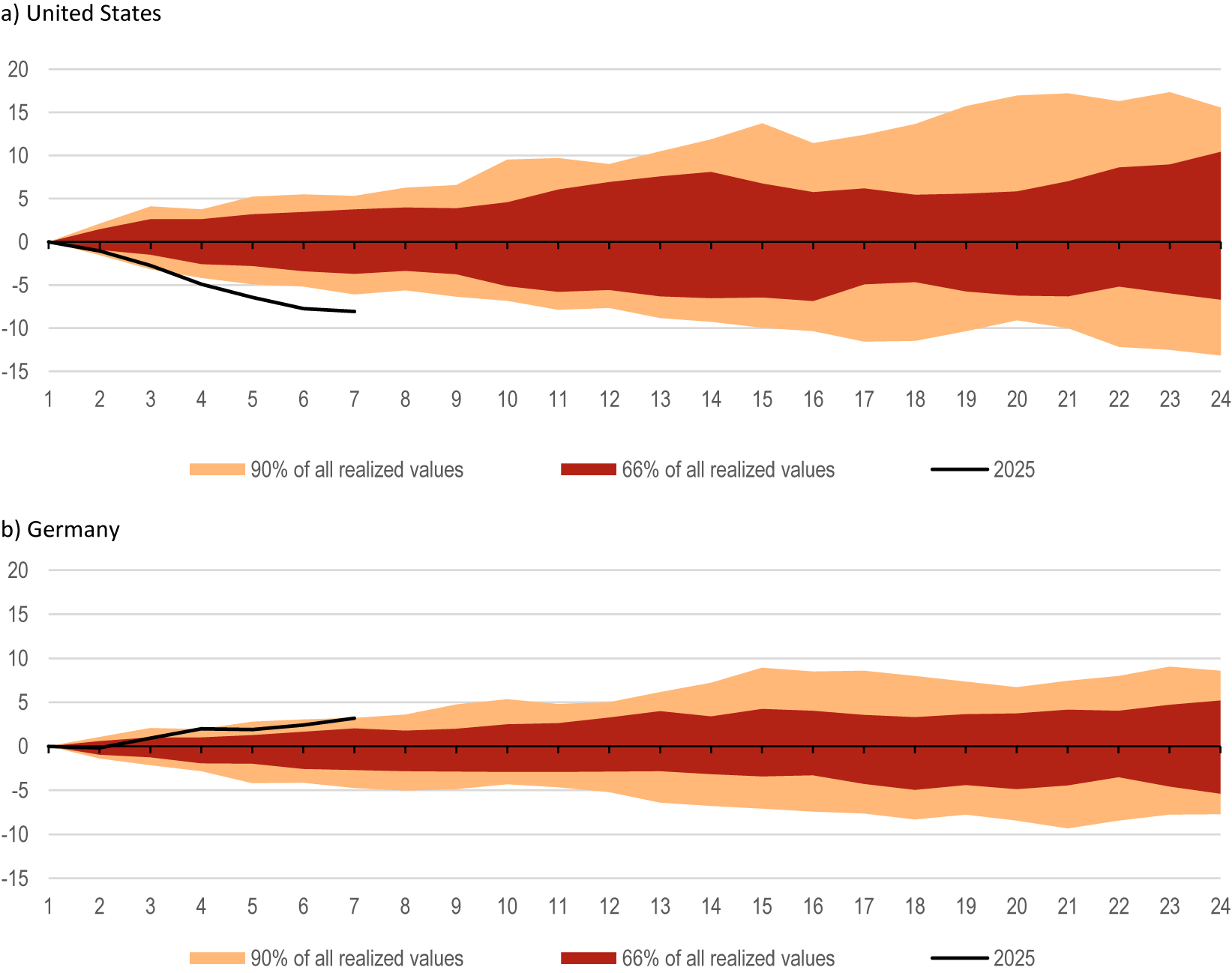
Since the new administration took office in early 2025, the US dollar has declined by 13.3% against the euro, 13.7% against the Swiss franc and 6.7% in nominal effective terms. This sharp depreciation of the US dollar reflects shifting economic expectations—namely, a modest recovery in the German economy and a slowdown in the previously booming US economy—as well as a loss of confidence in the US currency. While the dollar continues to serve as the world’s primary reserve currency, its recent depreciation exceeds what would typically be considered normal exchange rate fluctuations (Figure 1).
Real effective exchange rate since 1982. Cumulative percentage change year to date, %, monthly, narrow index. The figure shows overlapping paths of the real effective exchange rate against 51 countries over 24 months. The length of the paths was chosen based on exchange rate developments in the 1980s, also referred to in Miran (Reference Miran2024). Until 1985, the US dollar appreciated strongly—by 12% in real effective terms over 2 years because restrictive monetary policy and increased government borrowing led to rising US interest rates resulting in higher global investments in the US. In 1985, the Plaza Accord between representatives of the G5 countries resulted in foreign exchange interventions and a 15% real effective depreciation of the dollar by 1987
Source: Bruegel via Macrobond, authors’ calculations.

Figure 1. Long description
The graph consists of two vertically stacked panels, a and b. Both panels share a horizontal x-axis representing months from 1 to 24 and a vertical y-axis representing cumulative percentage change from negative 15 to 20 percent.
Panel a, titled United States, shows a wide fan chart. The innermost layer, shaded dark red, represents 66 percent of all realized values and expands symmetrically from 0 to approximately plus or minus 8 percent by month 24. The outer layer, shaded orange, represents 90 percent of all realized values and expands further, reaching approximately plus 15 percent and negative 13 percent by month 24. A solid black line labeled 2025 begins at month 1 and trends downward, reaching approximately negative 8 percent by month 7.
Panel b, titled Germany, shows a narrower fan chart compared to the United States. The dark red 66 percent interval expands to approximately plus 5 and negative 5 percent by month 24. The orange 90 percent interval expands to approximately plus 9 and negative 8 percent by month 24. A solid black line labeled 2025 begins at month 1 and trends slightly upward, reaching approximately plus 3 percent by month 7.
This article proceeds as follows. Section 2 identifies the key drivers behind the dollar’s recent decline. Section 3 draws on invoicing and reserve currency data to show that the dollar’s global role remains intact for now. This status is at risk, however, as discussed in Section 4. Against the backdrop of recent exchange rate dynamics, we use the NiGEM global macroeconomic model in Section 5 to simulate a sharp dollar depreciation under three scenarios: (1) a combined shock to the currency and investment risk premium; (2) a broad-based currency risk premium shock and (3) a currency risk premium shock specifically favouring the euro. In the first scenario involving cross-asset shocks, global growth slows, with the US economy most severely affected. In contrast, the other two scenarios indicate that a weakening of the US dollar could substantially benefit the Euro Area, provided the euro strengthens its role as an international reserve currency. In addition to acknowledging the model’s limitations, we also emphasise that a broader international financial crisis—triggered by a sharp loss of confidence in the US dollar—cannot be ruled out beyond the scope of NiGEM. Section 6 concludes and emphasises that for the Euro Area to benefit from a weaker US dollar, long-overdue reforms are needed to expand the supply and liquidity of Euro Area government bonds that qualify as safe assets.
2. Perceived risk of US dollar assets rises in 2025
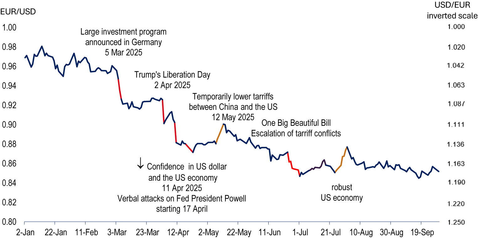
Two key factors contributed to the dollar’s depreciation in the first half of 2025: revised GDP growth expectations and a reassessment of the risk associated with the dollar and US Treasuries. Against the euro, the dollar had strengthened to 1.035 USD/EUR in January 2025—a level previously recorded only in the early 2000s and the second half of 2022. This was largely driven by Germany’s prolonged economic weakness since 2022 and heightened political uncertainty following the collapse of its coalition government in November 2024. However, the announcement of a planned investment initiative in early March 2025 improved Germany’s economic outlook and shifted expectations for monetary policy, prompting an appreciation of the euro to 1.086 USD/EUR within days of the announcement (Figure 2). The euro’s appreciation was accompanied by an increase in Germany’s long-term yields and a concurrent narrowing of the yield differential between the US and Germany.
Daily US dollar/Euro exchange rate, January to September 2025.
Source: ECB; authors’ calculations and dating.

Figure 2. Long description
The X axis represents time from 2-Jan to 19-Sep 2025. The left Y axis shows E U R forward slash U S D values from 0.80 to 1.00. The right Y axis shows an inverted U S D forward slash E U R scale from 1.250 to 1.000. The data line begins near 0.97 in January and shows a volatile but steady decline. Key annotations include:
* 5 Mar 2025: Large investment program announced in Germany, coinciding with a peak near 0.96.
* 2 Apr 2025: Trump's Liberation Day, followed by a sharp red-colored drop to 0.92.
* 11 Apr 2025: Downward arrow indicating Confidence in U S dollar and the U S economy.
* 17 April: Verbal attacks on Fed President Powell starting, followed by another red-colored decline.
* 12 May 2025: Temporarily lower tariffs between China and the U S, marked by an orange-colored upward correction to 0.90.
* June to July: Escalation of tariff conflicts and One Big Beautiful Bill, marked by a red-colored drop to approximately 0.85.
* Late July: Robust U S economy annotation during an orange-colored recovery.
* August to September: The rate stabilizes and fluctuates between 0.85 and 0.86.
The depreciation of the US dollar in subsequent months was primarily driven by domestic events. At times, the dollar weakened even as long-term interest rates rose—indicating a rising risk premium and a loss of investor confidence in the currency. This was most pronounced following the sweeping global tariff declaration on Trump’s so-called ‘Liberation Day’, when the dollar fell by nearly 3% against the euro. The S&P 500 dropped by 12% over the next four trading days. Although equity markets recovered significantly within 9 days—largely due to the temporary suspension of most tariffs on April 9—the dollar had declined by a total of 5% against the euro, reaching 1.135 USD/EUR. Over the same period, the yield on the US 10-year Treasury rose by 0.3 percentage points, while its German counterpart declined by 0.1 percentage points.
The dollar reached a preliminary low of 1.15 USD/EUR on 22 April 2025, following repeated criticism by Trump of Federal Reserve Chair Powell and hints at his potential dismissal. Shifts in short-term interest rate expectations suggest that the depreciation of the dollar and the corresponding decline in the foreign-currency value of dollar-denominated assets partly reflect concerns about a weaker medium-term US economic outlook. By 22 April, the federal funds rate expected for December 2025 was 0.5 percentage points lower than on 20 February and 0.6 points lower for maturities through December 2029. However, the 10-year US-German bond yield spread stood at 1.97 percentage points—the same level observed on 1 November 2024 and 20 February 2025, when the exchange rate was significantly stronger at 1.089 USD/EUR and 1.044 USD/EUR, respectively. Meanwhile, long-dated futures (March 2030) priced the euro at 1.240 USD/EUR, up from 1.109 USD/EUR (20 February) and 1.144 USD/EUR (1 November), both for December 2027 delivery. This indicates a revaluation of US bonds that cannot be explained by interest rate expectations alone.
A confidence-driven component is also suggested by the fact that the US dollar depreciated most sharply against the euro and the Swiss franc, that are typically also regarded as safe havens (Table 1).
Major US dollar exchange rates

Table 1. Long description
The table displays U S dollar per currency unit for three time points in 2025: January, July, and September, including percentage changes relative to January. A higher value indicates a depreciation of the U S dollar.
* Euro: Jan 1.0354; Jul 1.1677 (12.8% change); Sep 1.1732 (13.3% change).
* Japanese yen: Jan 0.00639; Jul 0.00679 (6.3% change); Sep 0.00676 (5.9% change).
* Pound sterling: Jan 1.2354; Jul 1.3489 (9.2% change); Sep 1.3514 (9.4% change).
* Canadian dollar: Jan 0.6950; Jul 0.7304 (5.1% change); Sep 0.7233 (4.1% change).
* Renminbi yuan: Jan 0.1371; Jul 0.1394 (1.7% change); Sep 0.1404 (2.4% change).
* Swiss franc: Jan 1.0994; Jul 1.2517 (13.9% change); Sep 1.2500 (13.7% change).
Source: Deutsche Bundesbank, F R E D Database, authors’ calculations.
Source: Deutsche Bundesbank, FRED Database, authors’ calculations.
1 A higher value indicates a depreciation of the US dollar.
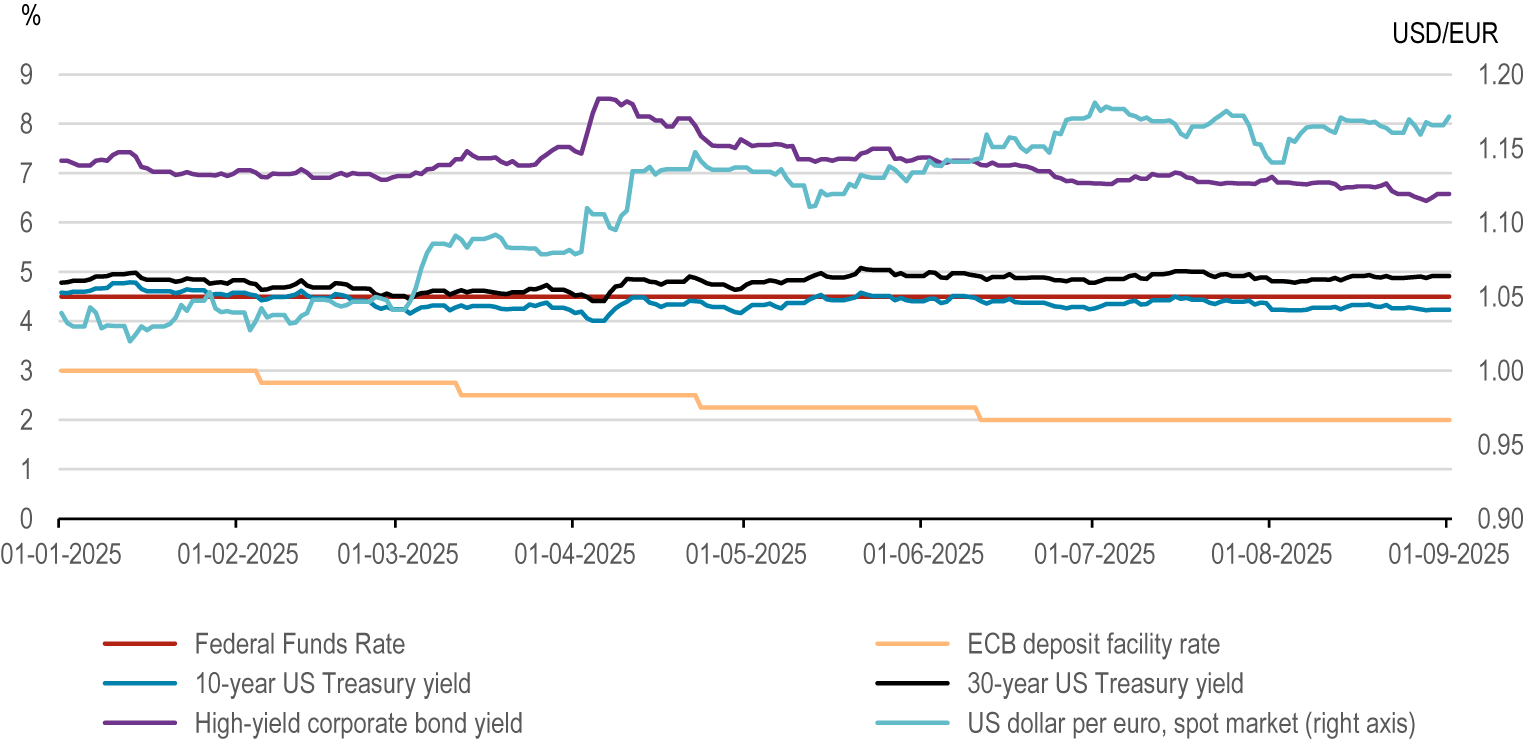
The marked increase in interest rates on high-risk bonds issued by US companies after 2 April 2025 also indicates a rise in the risk premium. Although these rates have since declined, a sustained upward trend is particularly evident for long-term US government bonds (Figure 3).
Diverse asset class indicators: policy, sovereign, corporate, and FX in 2025.
Source: Macrobond; Ice Data Indices; LLC via FRED; authors’ calculations.

Figure 3. Long description
The X-axis represents time from 01-01-2025 to 01-09-2025. The left Y-axis measures percentage from 0 to 9. The right Y-axis measures U S D forward slash E U R from 0.90 to 1.20.
* Federal Funds Rate (red line): Remains constant at approximately 4.5 percent throughout the period.
* 10-year U S Treasury yield (blue line): Fluctuates slightly between 4 and 5 percent, ending near 4.2 percent.
* High-yield corporate bond yield (purple line): Starts at 7.2 percent, peaks at 8.5 percent in April, then gradually declines to 6.5 percent.
* E C B deposit facility rate (orange line): Follows a downward step-wise pattern, starting at 3 percent and dropping to 2 percent by July.
* 30-year U S Treasury yield (black line): Remains relatively stable between 4.5 and 5 percent.
* U S dollar per euro, spot market (light blue line, right axis): Starts at 1.05, shows significant volatility with a sharp rise in April, peaking near 1.18 in July, and ending around 1.16.
Since early July 2025, dollar exchange rates have moved little. In September 2025, the dollar-euro exchange rate stood at 1.173 USD/EUR, compared to 1.167 USD/EUR 2 months earlier. At the same time, the perceived risk of US dollar assets declined, as reflected in the substantial drop in the 10-year government bond yield differential between the US and Germany—from 1.72 percentage points in July to 1.41 percentage points in September. This marks a clear departure from the period between March and June 2025, when the dollar weakened from 1.081 USD/EUR to 1.152 USD/EUR and the yield differential widened from 1.50 to 1.84 percentage points, suggesting heightened risk perceptions and a revaluation of US dollar-denominated assets, given that depreciation of the US dollar and other advanced economy currencies is typically associated with a narrowing, rather than a widening, of the yield differential.
3. The US dollar’s slowly waning role as global key currency
The US dollar has been the dominant international currency for over 80 years, with the US meeting all the core requirements of a key currency country: The US economy was sufficiently large to play a sizable role in global markets; its political structures were sufficiently stable and transparent, and the market for safe assets—typically sovereign bonds, such as US Treasuries—was adequately deep and liquid as well as globally accessible. In addition, the US maintained a leading position in military power, technological innovation and productivity.
As the key currency country, the United States enjoys the ‘exorbitant privilege’ of being able to incur debt at lower interest rates than other sovereigns while investing abroad at higher yields (Eichengreen, Reference Eichengreen2010; Gourinchas and Rey, Reference Gourinchas and Rey2022).Footnote 1 This advantage stems from the strong global demand for the key currency country’s government bonds, which are widely held as currency reserves and other forms of reserves. Crucially, this demand is underpinned by the dominance of the key currency in invoicing global trade.
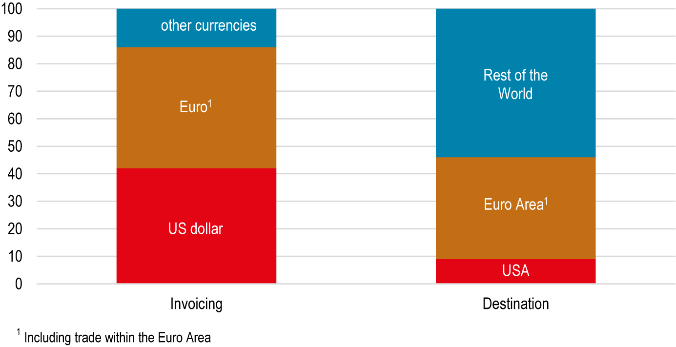
Not only are 94.8% and 95.8% of US imports and exports invoiced in US dollars, respectively (BIS, 2025), but the dollar also accounts for 60% of total exports worldwide (ECB, 2025). In contrast, the euro represents 25% of global export invoicing. When foreign trade within the Euro Area is included, the dollar and euro each account for approximately 40% (Boz et al., Reference Boz, Casas, Georgiadis, Gopinath, Le Mezo, Mehl and Nguyen2022; ECB, 2025). However, as illustrated in Figure 4, the share of exports invoiced in euros is only marginally higher than the share of Euro Area exports in global exports, whereas the US dollar’s share as an invoicing currency far exceeds the proportion of US exports in global exports.
Global export shares by invoicing currency and destination in %. Also see Eurostat (2025).
Source: ECB, 2025, p. 52; authors’ footnote.

Figure 4. Long description
A stacked bar chart with a Y-axis ranging from 0 to 100 in increments of 10. The X-axis has two categories: Invoicing and Destination.
Invoicing Bar (Left):
- Bottom segment (red): U S dollar, approximately 42%.
- Middle segment (orange): Euro super 1, approximately 44%.
- Top segment (blue): other currencies, approximately 14%.
Destination Bar (Right):
- Bottom segment (red): U S A, approximately 9%.
- Middle segment (orange): Euro Area super 1, approximately 37%.
- Top segment (blue): Rest of the World, approximately 54%.
A footnote at the bottom states: 1 Including trade within the Euro Area.
These proportions have remained largely unchanged since 1999 (Boz et al., Reference Boz, Casas, Georgiadis, Gopinath, Le Mezo, Mehl and Nguyen2022). The Chinese yuan has thus far played a minor role in global trade invoicing, accounting for less than 2% (ECB, 2025, p. 55). However, the Chinese government is eager to increase its role, and the potential for change is considerable given the size of China’s GDP and its significance in Asia and the global economy.
The importance of the US dollar in international trade invoicing drives strong demand for dollars, as imports must be paid for and reserves are accumulated accordingly, typically held in short-term Treasuries.
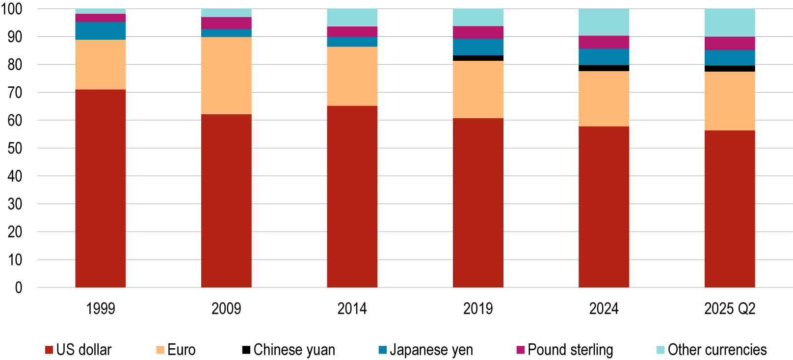
Accordingly, the dollar continues to dominate global currency reserves. In the first decade following the introduction of the euro, there was widespread expectation that it would partially replace the US dollar as the leading reserve currency (Timmer et al., Reference Timmer, Dailami, Irving, Hauswald and Masson2011). However, the Euro Area crisis revealed significant institutional weaknesses within the Euro Area—most notably, the lack of breadth and depth in the market for safe government bonds. By 2009, the euro’s share of international currency reserves had risen by 9.8 percentage points to 27.7%, while the US dollar’s share had declined by 8.9 percentage points to 62.2%.Footnote 2 The euro’s share then declined to 19% by 2015 and has since fluctuated between 19% and 21%, only slightly above its level at the time of introduction (Figure 5).
Currency composition of official currency reserves shares in %. In US dollars and without unallocated foreign exchange reserves.
Source: IMF, Currency Composition of Official Currency Reserves (COFER), 1 October 2025; authors’ calculations

Figure 5. Long description
The Y-axis represents the percentage share from 0 to 100 in increments of 10. The X-axis lists the years 1999, 2009, 2014, 2019, 2024, and 2025 Q 2.
Each bar is composed of six categories, described here from bottom to top:
* U S dollar (red): Starts at approximately 71 percent in 1999, fluctuates, and ends at roughly 56 percent in 2025 Q 2.
* Euro (orange): Starts at approximately 18 percent in 1999 and remains relatively stable, ending at about 21 percent in 2025 Q 2.
* Chinese yuan (black): First appears as a visible segment in 2019 at approximately 2 percent and remains at roughly 2 to 3 percent through 2025 Q 2.
* Japanese yen (dark blue): Maintains a consistent share of approximately 5 to 6 percent across the period.
* Pound sterling (magenta): Maintains a consistent share of approximately 3 to 5 percent across the period.
* Other currencies (light blue): Grows from approximately 2 percent in 1999 to roughly 10 percent by 2025 Q 2.
The overall trend shows a diversification of reserves away from the U S dollar toward other currencies and the Chinese yuan.
The share of the US dollar in international currency reserves has declined by 13 percentage points since 1999. Of this decline, approximately two percentage points each can be attributed to the euro, the pound sterling, and the Chinese yuan—the latter having been included in the IMF’s official reserve currency statistics only since 2016. An additional eight percentage points have shifted to ‘other currencies’, most notably the Australian dollar and the Canadian dollar, while the Japanese yen has lost just under one percentage point. The likely future tripolar currency system, comprising the dollar, the euro and the yuan, is still in its early stages. The dollar continues to serve as the dominant international reserve currency, albeit in a slightly diminished capacity, while the euro and the yuan function primarily as regional reserve currencies.
4. Risks to the US dollar from economic policy and geopolitical fragmentation
The geopolitical shifts of the past 3 to 10 years, along with the economic policy agenda of the Trump administration, increase the risk that the gradual decline in the dominance of the US dollar could give way to abrupt shifts away from Treasuries and possibly US assets more broadly. Potential consequences range from a sharp depreciation of the dollar to an international financial crisis.
As a result of the sanctions against Russia and rising geopolitical tensions more broadly, trade among the BRICS+ countries has not only intensified, but a payment system independent of the US dollar has also emerged. Given that the BRICS+ countries account for 45% of the world’s population and nearly 27% of global GDP (in US dollars),Footnote 3 the potential loss for the US dollar as both an invoicing and reserve currency is substantial.
Current US economic policy is likely to accelerate the decoupling of the BRICS+ countries from the US dollar and could also prompt other institutional and private investors to shift out of dollar-denominated assets. Central to this are the heightened uncertainty caused by Trump’s drastic and erratic tariff policy as well as his calls for significant interest rate cuts and a weaker dollar. Specifically, the Mar-a-Lago Accord—proposed by Stephen Miran, Chairman of the Council of Economic Advisers and appointed to the Federal Reserve Board of Governors in August 2025—has increased the risk of financial losses (Miran, Reference Miran2024). Miran’s narrative is that providing a reserve currency is not an ‘exorbitant privilege’ but rather a ‘burden’ as the high demand for US dollars and US dollar-denominated bonds leads to an overvaluation of the dollar that undermines export competitiveness and causes deindustrialisation (Krugman, Reference Krugman2025). His goal is to establish an exchange rate favourable to US manufacturing while maintaining low interest rates and simultaneously preserving the dominant position of the dollar. Failing voluntary acceptance of lower yields on US Treasuries and a weaker dollar by the beneficiaries of US hegemonic power, the US would enforce a conversion of Treasuries into 100-year bonds bearing little or no interest through the threat of tariffs and the withdrawal of military support. Trump’s backing of this position has created an environment in which investors must repeatedly question whether they can reallocate their US holdings ahead of a potential sell-off.
4.1. The nature of the shock matters
To assess the macroeconomic impact of large dollar depreciations, we use the NiGEM multi-country macroeconometric model, widely used by central banks. In NiGEM, exchange rates are modelled according to the risk-adjusted uncovered interest parity hypothesis, which holds that expected exchange rate changes reflect interest rate differentials and the currencies’ risk premia (Gandolfo Reference Gandolfo2001; Kirby and Meaning Reference Kirby and Meaning2014):

where fxt is the exchange rate at time, rt and
$ {r}_t^{us} $
 are the respective policy rates and
$ {\varepsilon}_t $
 is the relative country-specific risk premium. This relationship is derived from interest rate arbitrage between domestic and foreign investments, which requires that returns on comparable investments in different currencies be equal after adjusting for the risk premium (εₜ), reflecting their differing risk profiles and underlying currencies (Engel et al., Reference Engel, Pak and Wu2023; Kalemli-Özcan and Varela, Reference Kalemli-Özcan and Varela2021; Obstfeld and Zhou, Reference Obstfeld and Zhou2023).Footnote
4
Otherwise, arbitrageurs would exploit existing profit opportunities that subsequently vanish due to corresponding price adjustments.
The impact of exchange rate changes on macroeconomic variables like inflation and GDP growth depends on whether the shock stems from an expected change in monetary policy rates or from a change in risk premia, specifically a loss of confidence (Haincourt, Reference Haincourt2018, Table 2).Footnote 5
Impact of two different exchange rate shocks on GDP and Inflation 2025–2028

Table 2. Long description
The table analyzes a 10 percent depreciation occurring in the fourth quarter of 2025, comparing two causes: a U S rate cut and a higher risk premium. All values represent a deviation from the baseline.
Short-term effect in the U S (2026 Q 1):
* Inflation (percentage points): 2.3 for U S rate cut, 2.1 for higher risk premium.
* G D P (percent): 0.2 for U S rate cut, minus 0.5 for higher risk premium.
Medium-term effect in the U S (2028 Q 4):
* Inflation (percentage points): 1.1 for U S rate cut, 0.2 for higher risk premium.
* G D P (percent): 1.0 for U S rate cut, minus 1.7 for higher risk premium.
Source: Authors calculations using NiGEM.
Source: Authors’ calculations using NiGEM.
The short-term effect on inflation is similar in both cases because the exchange rate pass-through is the same. The exchange-rate elasticity of inflation depends on (i) the impact of the exchange rate (ER) on import prices and (ii) the pass-through (PT) of import prices to inflation. In the empirical literature, the first part is typically identified as inelastic and smaller than 1. Furthermore, the reaction of import prices is quick but varies across countries and products due to microeconomic factors such as margin behaviour and currency invoicing. The second part of the transmission channel also differs across countries, largely depending on the import intensity of GDP. In the medium term, the inflation impact differs significantly between the two scenarios: the increase in GDP following the rate cut fuels inflation, whereas the risk premium-induced decline in GDP curtails it.
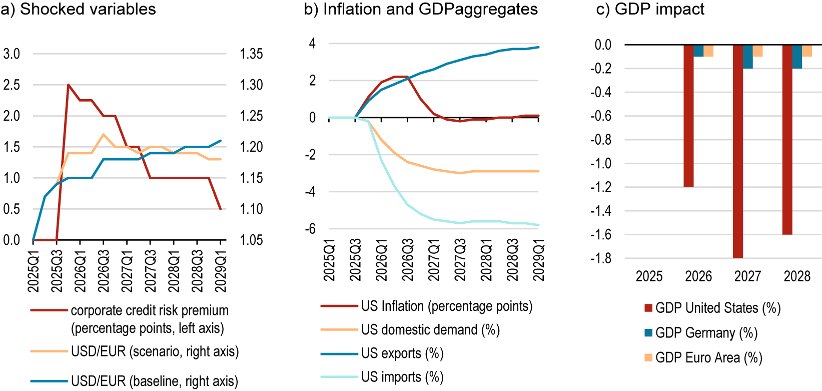
In the following, we discuss the results of three depreciation scenarios related to a loss of confidence in the US dollar. The depreciation is modelled as an increase in the US dollar risk premium from the fourth quarter of 2025 until the end of Donald Trump’s second term in the fourth quarter of 2028) (Figures 6 and 7).
Loss of confidence in the US dollar across asset classes (Scenario 1).
Deviation from baseline after shock to exchange rate and investment risk premium.
Source: Authors’ calculations using NiGEM.

Figure 6. Long description
Panel a, Shocked variables, is a line graph with time from 2025 Q 1 to 2029 Q 1 on the X axis. The left Y axis measures percentage points from 0.0 to 3.0 for corporate credit risk premium, which peaks at 2.5 in late 2025 before declining to 0.5. The right Y axis measures U S D forward slash E U R exchange rates from 1.05 to 1.35. The baseline rate increases steadily to 1.20, while the scenario rate peaks at 1.22 in 2026 before stabilizing near 1.18.
Panel b, Inflation and G D P aggregates, uses a Y axis from minus 6 to 4. U S exports show a steady climb to nearly 4 percent. U S inflation peaks at 2 percentage points in 2026 then returns to 0. U S domestic demand and U S imports both drop sharply in 2025, with imports stabilizing at minus 6 percent and demand at minus 3 percent.
Panel c, G D P impact, is a bar chart showing annual percentage deviations for 2026, 2027, and 2028. The U S G D P shows the largest negative impact, reaching minus 1.8 percent in 2027. Germany and the Euro Area show smaller negative impacts, both remaining between 0.0 and minus 0.2 percent.
Scenarios with currency-only risk premium shock.
L, left axis; R, right axis; pp, percentage points; NEER, nominal effective exchange rate; current account in % of GDP.
Source: Authors’ calculations using NiGEM.

Figure 7. Long description
The figure is divided into two horizontal sections: Scenario 2 (Uniform Depreciation) and Scenario 3 (Depreciation Favoring the Euro). Each section contains three panels.
Scenario 2:
Panel a, Shocked variables: A line graph with time on the x-axis from 2025 Q 1 to 2029 Q 1. The left y-axis measures percentage deviation and the right y-axis measures exchange rate. U S N E E R (red line) drops sharply from 0 to -10.5. U S D / E U R scenario (orange line) rises from 1.15 to 1.28, while the baseline (blue line) rises more gradually to 1.20.
Panel b, Inflation and G D P aggregates: Euro Area inflation (red) dips to -1.0 p p before recovering to 0. Euro Area consumption (orange) rises to 0.6%. Current account balance (purple) stays near 0.1 p p. Euro Area investment (blue) on the right axis rises from 0 to 2.5%.
Panel c, G D P impact: A bar chart showing annual data from 2025 to 2028. G D P U S (red) shows a negative impact reaching -1.6%. G D P Germany (blue) and G D P Euro Area (orange) show positive impacts reaching 0.6% and 0.7% respectively.
Scenario 3:
Panel a, Shocked variables: Similar to Scenario 2, but the U S N E E R (red) drop is slightly less severe, ending near -9.0. The U S D / E U R scenario (orange) reaches a higher peak of 1.35.
Panel b, Inflation and G D P aggregates: Euro Area inflation (red) sees a much deeper initial drop to -2.8 p p before recovering. Euro Area consumption (orange) and investment (blue) show stronger growth, with investment reaching nearly 9.0% on the right axis. Current account balance (purple) turns negative, reaching -0.8 p p.
Panel c, G D P impact: G D P U S (red) remains negative at -1.4%. G D P Germany (blue) and G D P Euro Area (orange) show higher positive gains than Scenario 2, both approaching 0.9%.
4.2. Risk premium shock across asset classes (Simulation 1)
The most likely of the three scenarios is based on previously discussed market dynamics observed around 2 April 2025, which were characterised by heightened perceived risk not only towards the US dollar but also other dollar-denominated assets (Figure 3). We therefore shock both the investment risk premium and the exchange rate risk premium until the end of President Trump’s second term.Footnote 6 The size of the first shock is chosen to reflect twice the monthly market movements around Trump’s Liberation Day, i.e., the spread between March and April 2025. For high-yield bonds, the spread between April 10 and March 10 was just under 1.3 percentage points (Figure 3), resulting in a shock size of the corporate credit risk premium of 2.5 percentage points against the baseline (Figure 6). The choice of the scaling factor is subject to a certain degree of arbitrariness. However, doubling the spread does not cause market movements to fall outside a realistic range. In particular, the corresponding change in yields on high-yield bonds was far more pronounced during the 2008 financial market crisis (8 times) and at the start of the COVID-19 pandemic in 2020 (4 times). The choice of the shock size for the endogenous exchange rate risk premium shock follows a similar rationale. However, due to the combination and the nature of the shocks, the resulting magnitude in scenario 1 is not directly comparable.Footnote 7
In the simulation, the exogenous shock to the corporate loan risk premium outweighs the impact of the endogenous exchange rate risk premium shock. This is because the credit risk premium dampens corporate investment and weakens the US economy additionally, thereby mitigating the inflationary effect of the exchange rate shock. As a result, the Federal Reserve is able to lower rates again relatively quickly, which rapidly reduces the yield differential between the US and the Euro Area. Therefore, the exchange rate reverts towards its initial level and, by the end of the simulation period, even falls below it. In this scenario, by the end of Trump’s second term, the US dollar appreciates by 2 cents relative to the euro, after an initial depreciation of slightly more than 4 cents against the baseline (Figure 6a).
The temporary rise in inflation and the credit risk shock reduce both private consumption and investment. As a result of diminished purchasing power and higher interest rates, US domestic demand remains around 3% below the baseline forecast in the event of a loss of confidence across asset classes (Figure 6b). In the NiGEM model, US exports increase by 4% and imports decline by 6% relative to the baseline, reflecting the exchange rate-driven drop in the cost of US exports and rise in the cost of imports. However, the current account balance (as a percentage of GDP) improves by only just over 0.5 percentage points on average over the simulation period. In addition to net exports, the model also accounts for cross-border flows of primary and secondary income. Overall, US GDP falls up to 1.8% short of the baseline forecast (Figure 6c). In an isolated shock scenario without endogenous exchange rate shock, but with an identical temporary increase in the corporate credit risk premium, the maximum GDP loss would be just under 0.4%.
Notably, in this scenario of a broad-based loss of confidence in US dollar-denominated assets, the Euro Area also experiences a decline in growth. Initially, the non-US rest of the world benefits from cheaper imports due to the dollar’s depreciation, as in the other two scenarios that are limited to a loss of confidence in the currency market. Raw materials, and crude oil in particular, play a key role in this respect, as their prices are typically determined and invoiced in US dollars. As the additional credit market shock unfolds, the initially expansionary impact on the Euro Area is more than offset by the economic downturn in the US and the resulting decline in exports. Beyond the scope of the model, the impact of the shocks is likely to be more severe due to international spillover effects of the initially domestic financial market turmoil, especially in the case of the US (Dimpfl and Jung Reference Dimpfl and Jung2012). However, the welfare-reducing spillover effects in the NiGEM simulation remain comparatively small, as the Federal Reserve’s rapid monetary policy response leads to timely stabilisation without any interim turbulence. Overall, Euro Area GDP lies only 0.1% below the baseline in the years 2026 to 2028, with German GDP slightly lower at −0.2%. US GDP losses are substantially more pronounced, ranging from −1.6% to −1.8% over the period under consideration. Despite the additional credit risk shock, these losses are only slightly higher than in the scenario where the loss of confidence is limited to the foreign exchange market, as a result of the central bank’s decisive response. This outcome reflects the New Keynesian structure of the NiGEM model, which is not well-suited to modelling financial market crises.Footnote 8
A review of the literature reveals alternatives to modelling exchange rates in New Keynesian equilibrium models such as NiGEM. For example, Proaño (Reference Proaño2011) advocates a behaviour-oriented, agent-based approach in which foreign exchange trading is driven not only by agents conducting fundamental macroeconomic analysis, but also by speculators motivated by chart analysis. As a result, periods of calm with low exchange rate fluctuations alternate with turbulent periods of high volatility. The latter have the potential to trigger a financial market crisis that destabilises the broader economy. Given the complexity of financial markets, NiGEM is therefore likely to significantly underestimate the growth losses that could arise for the Euro Area and Germany from a cross-asset loss of confidence in the US dollar.
Another caveat is that the relevant parameters in NiGEM imply a strong inflationary impact from changes in the exchange rate. This can be most easily illustrated by the long-term relationship of the error correction specification of consumer prices as a weighted average of domestic and foreign prices:

where UTC describes domestic price dynamics (total unit costs) and PM describes import prices. Preliminary re-estimates for individual countries suggest that the sensitivity of consumer prices to import prices (1 – β), which are directly influenced by changes in the currency value, is lower than the NiGEM coefficient. However, re-estimating and revising the foreign trade structure of the model is beyond the scope of this article, so the results presented here rely on the original parameter values. Nonetheless, the impact of model uncertainty in this regard is clear: if the inflationary effect of exchange rate changes were smaller in our simulations, the growth losses in the US would likely be less severe. The opposite holds for the countries of the Euro Area.
4.3. Currency-only risk premium shocks (Simulations 2 and 3)
In contrast to the first scenario, which at least hints at a financial crisis, the second and third scenario reflect a less disruptive shift to a global multi-currency system.
The second scenario contemplates a significant and uniform depreciation of the US dollar against other currencies, thereby entailing an exchange rate of 1.28 US dollars per euro (Figure 7.1a). Similar to the first scenario, the US experiences higher inflation, elevated interest rates, significantly subdued domestic demand and slightly improved foreign trade. However, as the bond and credit markets are not subject to any shocks, the GDP loss relative to the baseline is slightly lower, peaking at 1.6%. Unlike the first scenario, Euro Area countries benefit from higher investment due to temporarily lower inflation, which allows the central bank to reduce key interest rates. Private consumption also increases noticeably (Figure 7.1b).
The third simulation shifts focus by assuming that a nominal effective depreciation of the US dollar—similar to that in the second scenario—results from a non-uniform depreciation of the US dollar against other currencies (Figure 7.2). The simulation now includes a depreciation of the US dollar to approximately 1.35 dollars per euro (Figure 7.2a), while all other currencies appreciate slightly less than before. The overall impact on US GDP is very similar to that in the previous scenario. However, at its peak, US GDP is now only 1.4% below the baseline level (Figure 7.2c). This simulation is more exploratory than the other two, as it is based on conditions that would require measures to increase the supply and liquidity of Euro Area safe assets. These conditions are discussed in greater detail in the conclusion.
Compared with the second scenario, Euro Area countries now fare even better. Following the ECB’s rate cuts, investment is 5% above baseline and private consumption is 1% above baseline due to gains in purchasing power (Figure 7.2b). Strong domestic demand causes the current account balance to fall slightly compared with the baseline (by 0.4 percentage points). The mechanisms inherent in the model prevent deflationary risks from materialising in this scenario. All in all, under the simulated conditions, Euro Area GDP would be 0.4% to 0.9% higher than in the baseline. For Germany, GDP gains would range between 0.6% and 0.9%, depending on the year.
5. Potential for Euro Area gains amid declining dollar dominance
Our first simulation highlights the risks to the global economy posed by an abrupt loss of confidence in the US dollar, while the exploratory third simulation highlights the euro’s potential as a global currency. The Euro Area could benefit from a diminished role of the US dollar as a global currency, provided that key conditions are met to enhance the euro’s attractiveness as an international currency.
However, achieving this remains challenging for a ‘currency without a state’ (Eichengreen, Reference Eichengreen2010), as confidence in a currency rest not only on a credible, stability-oriented central bank, but also on a sovereign with solid public finances, whose debt offers a large and reliable supply of safe assets. The euro crisis of 2011–2012 revealed a fundamental weakness in the Euro Area: the government bonds of member states cannot be regarded as broadly substitutable safe assets. In its aftermath, the potential advantages of European bonds were widely discussed, including the possibility of strengthening the fiscal space of highly indebted countries while curbing moral hazard, jointly financing growth-enhancing investments (such as in digitalisation and climate action), stabilising financial markets, and increasing the Euro Area’s resilience to macroeconomic shocks. The latter is particularly important, as the dearth of safe government bonds leaves the Euro Area vulnerable to sudden shifts in expectations, which can trigger a vicious circle of rising risk premiums, higher private borrowing costs, falling output and capital flight (Theobald and Tober, Reference Theobald and Tober2020).
The Euro Area has evolved in recent years, notably through joint borrowing initiatives such as the NextGenerationEU program, the Eurosystem’s securities purchase programs, and the ECB’s new Transmission Protection Instrument. However, for the euro to play a stronger international role, additional steps are needed to develop a sufficiently broad and deep market for safe euro-denominated bonds. Currently, only the government bonds of Germany, the Netherlands, and Luxembourg hold top credit ratings. Politically, joint and several eurobonds, which could supplement the existing stock of safe bonds in the Euro Area, are not feasible at this time. Nonetheless, it has become clear that EU bonds issued by the European Commission may represent a viable alternative (Blanchard and Ubide, Reference Blanchard and Ubide2025).
The yield on EU bonds issued to finance NextGenerationEU at a remaining maturity of 10 years is only 0.4 percentage points above the yield on 10-year German government bonds and could be further reduced if these bonds gained the same status as sovereign bonds. Following Blanchard and Ubide (Reference Blanchard and Ubide2025), Euro Area countries could transfer a certain share of their existing sovereign debt to the EU and, in return, commit a corresponding share of their tax revenues for servicing this debt. Crucial for building trust is that no new debt is issued for this purpose; rather, existing debt should be converted into a new pool of safe euro-denominated EU bonds. This would also make the Euro Area more resilient to the risk of a financial crisis triggered by a major loss of confidence in the US dollar, a risk not to be underestimated even though we do not explicitly simulate such an event in this article.