1. INTRODUCTION
The ionosphere is a layer of the Earth's atmosphere between 50 and 2,000 km from the Earth's surface, and atoms that are potentially ionised due to solar energy are located in this layer. It has some permanent and regular changes of a temporal nature with periods such as diurnal, 27-day, seasonal, semi-annual, annual and 11-year. In addition, irregular changes in the ionosphere are caused by space weather conditions (solar effect, geomagnetic storms, etc), natural phenomena (earthquake, tsunami, volcanic explosions, etc) and anthropogenic events (rocket launches, nuclear explosions, etc). These changes are known as ionospheric disturbances and/or anomalies.
Investigation of seismic-related anomalies in the ionosphere has been ongoing for many years (Davies and Baker, Reference Davies and Baker1965; Weaver et al., Reference Weaver, Yuen, Prolss and Furumoto1970; Gokhberg, Reference Gokhberg1983; Molchanov et al., Reference Molchanov, Kopytenko, Voronov, Kopytenko, Matiashvili, Fraser-Smith and Bernardi1992; Pulinets, Reference Pulinets1998; Liu et al., Reference Liu, Chen, Chuo and Tsai2001; Pulinets et al., Reference Pulinets, Legen'Ka, Gaivoronskaya and Depuev2003; Liu et al., Reference Liu, Chen, Chen, Liu, Chen, Nishihashi, Li, Xia, Oyama, Hattori and Lin2009; Le et al., Reference Le, Liu, Liu, Zhao, Chen and Wan2013; Fidani, Reference Fidani2018). The first studies of seismo-ionospheric coupling reported on the Good Friday Alaska Earthquake of 1964 (Davies and Baker, Reference Davies and Baker1965; Leonard and Barnes, Reference Leonard and Barnes1965). The topic became more interesting and important with other subsequent studies showing the formation of ionospheric anomalies before strong earthquakes (Yuen et al., Reference Yuen, Weaver, Suzuki and Furumoto1969; Weaver et al., Reference Weaver, Yuen, Prolss and Furumoto1970). Satellite-based data for seismo-ionospheric studies was reported in the early 1980s (Gokhberg, Reference Gokhberg1983). Ongoing research utilised ground-based ionosonde data, Ultra Low Frequency/Low Frequency (ULF/LF) radio waves and ionospheric topside sounding (Liu et al., Reference Liu, Chen, Pulinets, Tsai and Chuo2000; Molchanov et al., Reference Molchanov, Kopytenko, Voronov, Kopytenko, Matiashvili, Fraser-Smith and Bernardi1992; Pulinets et al., 1998). Global Positioning System (GPS) technology was first applied in this study area on 17 January 1994, during the Mw =6 · 7 Northridge earthquake (Calais and Minster, Reference Calais and Minster1995).
As the ionospheric effect on radio signals through the atmosphere is inversely proportional to the square of the signal frequency, the free electron density in the ionosphere can be calculated through Global Navigation Satellite Systems (GNSSs) signals with different frequencies (Ciraolo et al., Reference Ciraolo, Azpilicueta, Brunini, Meza and Radicella2007). The free-electron count in the ionosphere is defined as the Total Electron Content (TEC). A TEC Unit (TECU) is defined as 1 TECU =1016 el/m2. Due to its advantages such as low-cost, high accuracy, near real-time and continuity, Global Positioning System (GPS)/GNSS technology is used in many large earthquakes to investigate seismo-ionospheric coupling (Yiyan et al., Reference Yiyan, Yun, Xuejun and Xunxie2009; Yao et al., Reference Yao, Chen, Wu, Zhang and Peng2012; Le et al., Reference Le, Liu, Liu, Zhao, Chen and Wan2013; Guo et al., Reference Guo, Li, Yu, Liu, Zhao and Kong2015a; Li et al., Reference Li, Meng, You, Zhang, Shi and Han2015). Le et al. (Reference Le, Liu, Liu, Zhao, Chen and Wan2013) utilised GPS-TEC data to investigate the ionospheric disturbances before the 2011 Tohoku-Oki earthquake. A significant enhancement was detected in TEC variation on 8 March 2011, when solar activity also showed a large increase. The results showed that not only the solar radiation enhancement was not enough to produce the observed significant TEC enhancement but also some additional mechanisms, such as pre-earthquake ionospheric disturbance or geomagnetic activities may have played a significant role in the TEC enhancement on 8 March. Guo et al. (Reference Guo, Li, Yu, Liu, Zhao and Kong2015a) analysed the impending ionospheric anomalies before the Iquique Mw8·2 earthquake in Chile on 1 April 2014. A sliding interquartile range with a 27-day window was applied to TEC data to eliminate effects of the solar and geomagnetic activities. The results showed that the TEC over the epicentre increased with an amplitude of 15 TECU, and the duration exceeded six hours on the fifth day before the earthquake. The F2 layer critical frequency (foF2) data was not affected by the magnetic activities, but the TECs were moderately affected by anomalous magnetic activity during some periods of the fifth day prior to the earthquake according to cross-wavelet analysis. Li et al. (Reference Li, Meng, You, Zhang, Shi and Han2015) identified ionospheric anomalies related to the 12 May 2008, Ms8·0 Wenchuan earthquake using GPS-TEC, ionosonde, Global Ionosphere Map-vertical Total Electron Content (GIM-vTEC) and electron density profiles detected by the Constellation Observation System for Meteorology Ionosphere and Climate (COSMIC). They found that a unique positive anomaly in TEC, recorded at 16 GPS stations, appeared on 9 May 2008. The ionosonde and COSMIC data revealed a characteristic similar to GPS TEC variations. The GIM showed that the anomalous variations of 9 May were located southeast of the epicentre. Results showed that the detected anomalies on 9 May were probably an ionospheric precursor of the Wenchuan earthquake of 12 May 2008.
The pre-seismic and co-seismic ionospheric conditions of the Van earthquake have been studied in previous works (Arikan et al., Reference Arikan, Deviren, Lenk, Sezen and Arikan2012; Zolotov et al., Reference Zolotov, Namgaladze and Prokhotov2012; Roland et al., Reference Roland, Vergnolle, Nocquet, Sladen, Dessa, Tavakoli, Nankali and Cappa2013; Alcay, Reference Alcay2016). Arikan et al. (Reference Arikan, Deviren, Lenk, Sezen and Arikan2012) investigated GPS-TEC values obtained from the Turkish National Permanent GNSS Network (TNPGN) stations using the symmetric Kullback-Leibler divergence method. According to the results, significant TEC variations were detected by the GPS stations within 150 km of the epicentre around eight to nine days prior to the earthquake. Zolotov et al. (Reference Zolotov, Namgaladze and Prokhotov2012) discussed the possible precursor of the Van earthquake using differential TEC maps relative to the quiet background conditions of the ionosphere. Strong long-lived TEC disturbances (~40%) were observed at the near-epicentre and magnetically conjugated areas between 20–23 October 2011 and reached the maximum level on 21 October, two days before the earthquake. Alcay (Reference Alcay2016) detected that the TEC obviously increased three days before, and two days after the Van earthquake using Precise Point Positioning (PPP)-based Regional Ionosphere Maps (RIM) and GIMs. It is stated that these positive anomalies should be related to seismic activity and a geomagnetic storm, respectively.
The ionosphere is affected instantaneously or periodically by Traveling Ionospheric Disturbances (TID), solar activity, magnetic storms and seasonal changes (Fejer and Scherliess, Reference Fejer and Scherliess1995). Nevertheless, the main phenomenon that causes ionospheric perturbation is solar activity, which also causes geomagnetic storms (Kutiev et al., Reference Kutiev, Tsagouri, Perrone, Pancheva, Mukhtarov, Mikhailov, Lastovicka, Jakowski, Buresova, Blanch, Andonov, Altadill, Magdaleno, Parisi and Torta2013). To establish a meaningful relationship between earthquake and ionosphere, it is necessary to distinguish some physical phenomena that cause a short-time ionospheric change from seismo-ionospheric coupling. For example, TID is a short-time distribution, which can be seen for about one to two hours in the ionosphere. So, seismo-ionospheric anomalies have been expected to be continuous for at least two hours. It is also questionable that the anomalies detected in the ionosphere are most likely to be caused by seismic activity when geomagnetic and solar activity is high. It is unrealistic to claim that anomalies of less than four to six hours are associated with an earthquake, especially when a geomagnetic storm is effective (Pulinets and Boyarchuk, Reference Pulinets and Boyarchuk2004). If the solar and geomagnetic conditions are quiet and anomalies continue for at least six hours, the corresponding day may be regarded as an abnormal day before an earthquake. It is also known that there is no significant change in the ionosphere when the solar and geomagnetic activity is quiet (Liu et al., Reference Liu, Chai, Liu, Chen and Chang2011).
The main motivation of this study is to detect the abnormalities in a TEC time series, which could be a precursor of an earthquake, using the STFT method and this method does not require any median, average or similar background value. For this purpose, GPS-TEC and GIM-vTEC variations with a time-span of 15 days before the Van earthquake were investigated. The methods of quartile-based running median process and STFT were utilised to determine anomalies in TEC variation. Regional ionosphere maps were generated to observe spatial distribution of anomalies using nine International GNSS Service (IGS) and 17 Turkish National Permanent Real-Time Kinematic (RTK) Network (TNPGN)-Active stations on 15, 16 and 21 October 2011. In addition, the Cross-Wavelet Transform (CWT) method was used to define the degree of correlation between solar activity and the anomalies because the anomaly days include high solar activity levels.
The remainder of this paper is organised as follows: in Section 2.1, detailed information of the Van earthquake is given. Section 2.2, covers the data observations. In Section 2.3, GIM-vTEC data of the epicentre is obtained, GPS-TEC data is calculated, and a short briefing of methods used in the study are shown. The results of the study are given in Section 3 and Section 4 concludes the paper.
2. DATA AND ANALYSIS
2.1. Van earthquake
A devastating earthquake occurred on 23 October 2011, at 10:41 Coordinated Universal Time (UTC) in the city of Van, Eastern Turkey. The disaster was one of the largest recent earthquakes in Turkey. The tectonic settings of the East Anatolia region of Turkey are the essential factors in earthquake occurrence. The movement rate of the Arabia plate towards the Eurasia plate is about 20–30 mm/year according to GPS measurements (Reilinger et al., Reference Reilinger, McClusky, Vernant, Lawrence, Ergintav, Cakmak, Özener, Kadirov, Guliev, Stepanyan, Nadariya, Hahubia, Mahmoud, Sakr, Abdullah, Paradissis, Al-Aydrus, Prilepin, Guseva, Evren, Dmitrotsa, Filikov, Gomez, Al-Ghazzi and Karam2006). Eastern Anatolia is a tectonically active region where the Arabian plate collides with the Anatolian plate leading to many strike-slip faults that vary in size and direction (Barka and Kadinsky-Cade, Reference Barka and Kadinsky-Cade1988). The earthquake rupture was unilateral towards the southwest indicating a reserve fault mechanism (Irmak et al., Reference Irmak, Doğan and Karakaş2012) confined to below a depth of 5 km, and it was dominated by a failure of a single asperity with a peak slip of about 5·5 m. The total seismic moment was calculated as 4 · 6 × 1019 Nm and the correspondingly moment Magnitude (Mw) was 7·1 (Utkucu, Reference Utkucu2012). The epicentre was estimated by the Kandilli Observatory and Earthquake Research Institute Regional Earthquake-Tsunami Monitoring Center (KOERI-RETMC) to be located at 38 · 7578°N, 43 · 3602°E, within a 15 km depth (KOERI, 2011).
2.2. Data observation
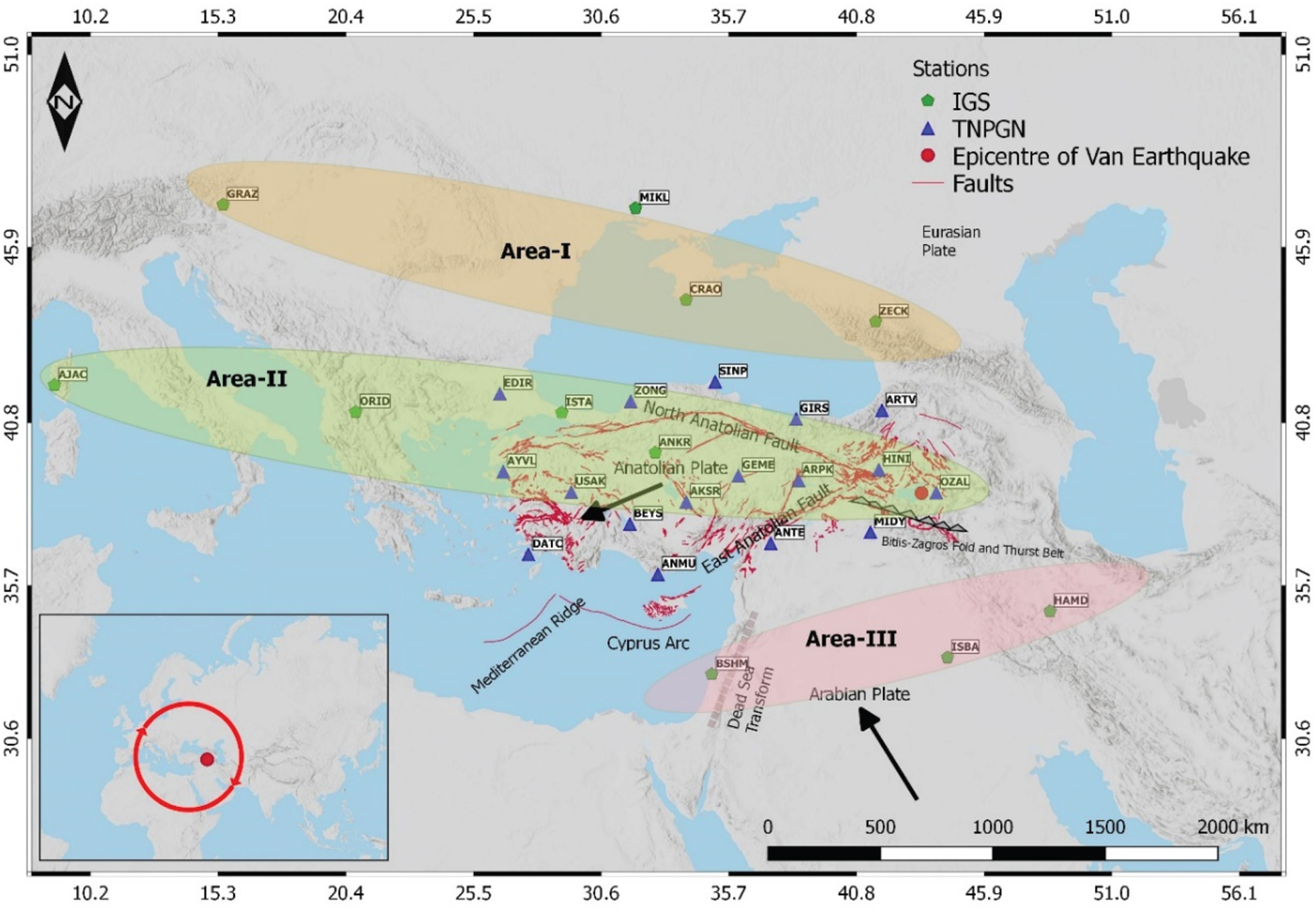
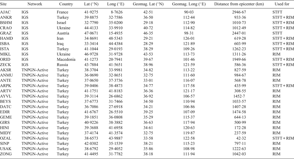
TEC data collected from 11 IGS and 17 TNPGN-Active stations and GIM-vTEC data obtained from the Center for Orbit Determination in Europe (CODE)-Global Ionosphere Maps (GIM) were used to detect uncommon ionospheric variations before the Van earthquake. The distribution of the stations and the epicentre are shown in Figure 1. Some attributes of the stations are listed in Table 1. In Figure 1, areas I-II and III indicate the stations, which are in approximately the same latitude and used for STFT analysis. In area-I, GRAZ, CRAO, ZECK stations, in area-II, AJAC, ORID, ISTA, ANKR, ARPK, OZAL stations and in area-III, BSHM, ISBA, HAMD stations were used for analysis. Receiver Independent Exchange Format (RINEX) files of the IGS stations were downloaded from the IGS website (ftp://igs.ensg.ign.fr/pub/igs/data/) and RINEX files of the TNPGN-Active stations were downloaded from the TNPGN-Active website (http://www.tusaga-aktif.gov.tr/default.aspx, ftp://212.156.70.42/) with a 30 second time resolution. CODE-GIM data was used to define the temporal variations of vTEC values at the epicentre. Ionosphere Map Exchange Format (IONEX) files were downloaded from the NASA website (ftp://cddis.gsfc.nasa.gov/gps/products/ionex/). The CODE-GIM data covers ± 87 · 5° latitude and ± 180° longitude ranges with 2 · 5° × 5° spatial resolution (5184 cells) and two-hour temporal resolutions. The time standard for data is selected as UTC and the Local Time (LT) for the city of Van can be calculated by LT = UTC +3 h.
The epicentre of the Van earthquake, IGS and TNPGN-Active stations.

Station information.

In order to analyse the effects of solar and geomagnetic activities on the anomalies, F10·7 solar flux, Kp, and Dst indices were utilised. The indices were downloaded from the OMNI website (https://omniweb.gsfc.nasa.gov/form/dx1.html). F10·7 solar flux is an important parameter to indicate the solar activity that defines the microwave flux density with a 10·7 cm wavelength. The unit of F10·7 is solar flux units (sfu) and when the solar activity is quiet, the value of F10·7 is generally below 70 sfu (Guo et al., Reference Guo, Li, Liu, Wang, Chang and Zhao2015b). Disturbance storm time (Dst) data with a one hour time resolution is used to represent geomagnetic activity in the low- and mid-latitude regions. Dst values are between −20 and 20 nanoTesla (nT) indicating quiet geomagnetic conditions. The Dst index also indicates a moderate and large-scale magnetic storm when it is below −50 nT and below −100 nT, respectively (Cander and Mihajlovic, Reference Cander and Mihajlovic1998). The global geomagnetic activity is defined by the Kp index with a three hour time resolution. The Kp index takes a value between 0 and 9, and the geomagnetic activity is quite when the Kp index is less than 4 (Menvielle and Berthelier, Reference Menvielle and Berthelier1991).
2.3. Methods
2.3.1. Epicentre vTEC (GIM-vTEC) and station-wise TEC (GPS-TEC) calculation
The vTEC values of the epicentre are calculated from the nearest four GIM grid points using a simple four-point bivariate interpolation (Schaer et al., Reference Schaer, Gurtner and Feltens1998). A simple four-point formula is shown in Equation (1):
 $$vTEC\lpar {\lambda_e,\beta_e} \rpar = \left[ {\matrix{ {1 - m} & m \cr } } \right]\left[ {\matrix{ {vTEC_{00}} & {vTEC_{01}} \cr {vTEC_{10}} & {vTEC_{11}} \cr } } \right]\left[ {\matrix{ {1 - n} \cr n \cr } } \right]$$
 $$m=\vert \lambda_{e}-\lambda_{0} \vert /{\Delta \lambda }_{GIM}$$
 $$n=\vert \beta_{e}-\beta_{0} \vert /{\Delta \beta }_{GIM}$$
where βe and λ e are the geocentric latitude and longitude of the epicentre, β0 and λ0 are the geocentric latitude and longitude of the nearest grid point, Δβ GIM and Δλ GIM are the spatial resolutions of the latitude and longitude of the GIM and vTEC 00, vTEC 01, vTEC 10, vTEC 11 are the vTEC values of the nearest four grid points.
The Geometry-Free Linear Combination (L 4) of the L1 and L2 signals is used to calculate station-wise TEC values. The L 4 combination of the carrier phase observations can be written as:
 $$L_{4}=L_{1}-L_{2}=-\beta sTEC+\lambda_{1}B_{1,i}^{k}-\lambda_{2}B_{2,i}^{k}$$
where  $\beta = \alpha \left( {\displaystyle{1 \over {f_1^2 }}-\displaystyle{1 \over {f_2^2 }}} \right)$ is a constant and
 $\lambda_{1}\hbox{B}_{1\comma i}^{k}\comma \; -\lambda_{2}\hbox{B}_{2\comma i}^{k}$ is the initial phase ambiguity. The bias term
 $\lambda\hbox{B}_{i}^{k}$ is defined as follows (Schaer, Reference Schaer1999) (i and k indices refer to receiver and satellite respectively):
 $$\lambda B_{i}^{k}=\lambda \lpar N_{i}^{k}+\delta N_{i}^{k}\rpar +c(b^{k}+b_{i})$$
where λ is wavelength,  $\hbox{N}_{\rm i}^{\rm k}$ is an integer,
 $\delta\hbox{N}_{\rm i}^{\rm k}$ is the effect of the phase windup, c is the speed of light and b k, b i are hardware delays. The terms of the delays and the phases of the integer are not practically separated, and the unified term is called the ambiguity produced bias (Mannucci et al., Reference Mannucci, Wilson, Yuan, Ho, Lindqwister and Runge1998). Reducing ambiguities from L4, a “levelling carrier to code” algorithm is widely used. The procedure is based on differences of carrier and code ionospheric observable on a continuous arc (Ciraolo et al., Reference Ciraolo, Azpilicueta, Brunini, Meza and Radicella2007).
 $$P_{4}=P_{1}-P_{2}=\beta sTEC+c(\Delta b^{k}-\Delta b_{i})$$
 $$\langle L_{4,arc}+P_4\rangle_{arc} \cong \lambda_{1}\delta N_{1}-\lambda_{2}\delta N_{2}=B_{4}$$
 $$L_{4}=L_{4}+\langle L_{4,arc}+P_4\rangle_{arc}=\beta sTEC+b_{4}^{k}+b_{4,i}+B_{4}$$
In Equation (7), the L4 ionospheric observable is leveled with a bias that is produced by phase ambiguity. Finally, the slant Total Electron Content (sTEC) is formulated as Equation (9):
 $$sTEC=\beta^{-1}\lpar L_{4}-\lpar B_{4}+b_{4}^{k}+b_{4,i} \rpar \rpar $$
bk is satellite hardware delays and bi is receiver hardware delays (Differential Code Biases (DCB)) and can be supplied from IGS products, nevertheless receiver biases have to be estimated for stations not on the IGS network. The sTEC is calculated from Equation (9) for each satellite in any GPS observation epoch (Şentürk and Çepni, Reference Şentürk and Çepni2018). It is obtained along a ray path related to the length of the slant path. Therefore, the sTEC values are converted into the vTEC to define the electron density value at a certain point on the Earth. Although the ionosphere consists of several layers, the Single-Layer Model (SLM) is an assumption that all free electrons are gathered in a layer with an infinite thickness (Alizadeh et al., Reference Alizadeh, Schuh, Todorova and Schmidt2011). The sTEC values are converted to vTEC values using the SLM assumption and a mapping function.
 $$vTEC/sTEC \cong \cos {\varepsilon }^{\prime} = \sqrt {1 - {\left( {\displaystyle{{R_E} \over {R_E + h_m}}} \right)}^2{\cos }^2\varepsilon }$$
Equation (10) is a well-known mapping function for the calculation of the electron density in the vertical direction of the Ionospheric Pierce Point (IPP). The IPP is the intersection between the signal ray path and the SLM (Smith, Reference Smith2004). The projection of the IPP on the Earth is called the Sub-Ionosphere Point (SIP) (Boutiouta and Belbachir, Reference Boutiouta and Belbachir2006). In order to describe the electron density over a station, the TEC value is generally computed from the weighted average of the vTECs (Çepni and Şentürk, Reference Çepni and Şentürk2016).
 $$TEC = \left. {\displaystyle{{\sum\nolimits_{i = 1}^N {W_ivTEC_i} } \over {\sum\nolimits_{i = 1}^N {W_i} }}} \right|_{T_1}^{T_2} ;\quad \hbox{T}_1 - \hbox{T}_2\;\hbox{is time lapse interval}$$
In Equation (11), Wi indicates the weight of a satellite where i =0, 1, …, n and n are equal to all visible satellites at any epoch. Wi is generally described as a component of the satellite elevation angle.
2.3.2. The quartile-based running median process
The quartile-based running median process (Liu et al., Reference Liu, Chen, Chen, Liu, Chen, Nishihashi, Li, Xia, Oyama, Hattori and Lin2009) was applied to determine the TEC anomalies over 15 pre-earthquake days. The median  $\tilde{\hbox{M}}$ of every consecutive 15 days was calculated to find the divergence between the observed TEC on the sixteenth days and the median
 $\tilde{\hbox{M}}$. To determine the level of the divergence, the Lower Quartile (LQ) and the Upper Quartile (UQ) were computed. Under the assumption of a normal distribution with mean
 $\bar{\hbox{m}}$ and standard deviation σ for the TEC, the expected values of
 $\tilde{\hbox{M}}$ and LQ or UQ are
 $\bar{\hbox{m}}$ and 1 · 34 σ, respectively (Klotz and Johnson, Reference Klotz and J ohnson1983). To clarify an anomaly in the TEC values, the lower and upper bounds were defined as:
 $$LB=\tilde{{M}}-1{\cdot}5\lpar \tilde{{M}}-LQ \rpar $$
 $$UB=\tilde{{M}}+1{\cdot}5\lpar UQ-\tilde{{M}} \rpar $$
When an observed TEC on the sixteenth day exceeds its previous 15-day-based UB or LB, the positive or negative abnormal TEC signal is approved, respectively. The observed TEC value between the UB and LB defines no abnormal condition in the ionosphere.
The Percentage Relative Anomaly (PRA) values were also calculated to define the size of anomalies according to observed TECs.
 $$PRA(\% ) = \displaystyle{{Anomaly} \over {ObservedTEC}} \times 100$$
2.3.3. Short-time Fourier transform
Gabor (Reference Gabor1946) adapted the Fourier transform to analyse only a small section of a signal at a significant time. It can be also called a technique of “windowing” the signal (Burrus, Reference Burrus1995). STFT maps a signal into a two-dimensional function of time and frequency. It provides information about both when and at which frequencies a signal occurs. If the chosen window shifts over a time and the window's instantaneous time is represented as τ then STFT is calculated:
 $$STFT\lpar {\tau ,f} \rpar = \vint_{ - \infty }^{ + \infty } {f(t)g(t - \tau )e^{ - i\omega t}dt}$$
where f(t) is a TEC time series, g(t) is the window function, τ is a shifting time variable and ω is angular frequency. The Fourier transform of the product f(t) with the g(t) infers the STFT. In this study, a discrete STFT was applied to obtain a time-frequency map of the TEC variations. By this method, there will be a detailed opportunity to identify and collect the frequency anomalies in the time domain.
The well-known fast Fourier transform algorithm was performed and Fourier coefficients were estimated. Subsequently, STFT was implied by referring to the Gaussian window (Equation (16)) (Harris, Reference Harris1978; Auger and Flandrin, Reference Auger and Flandrin1995).
 $$g\lpar t \rpar = e^{ - 0\cdot 5{(\alpha \displaystyle{t \over {(N - 1)/2}})}^2}$$
where N is the length of the window and α could be termed as a frequency parameter.
The alpha (α) parameter that controls the frequency resolution at both extremities was taken as 0·005. The width of the window is inversely related to the value of α. A larger value of α produces a narrower window so the chosen α parameter gives relatively accurate resolution in the frequency domain.
2.3.4. Cross-Wavelet Transform (CWT)
Wavelet transforms, which expand time series into time-frequency space, can be used to find localised intermittent periodicities in a TEC time series. CWTs are also very often desirable for examining two time series together that may be expected to be linked in some way. In particular, to examine whether regions in time-frequency space with large common power have a consistent phase relationship and therefore are suggestive of causality between the time series (Grinsted et al., Reference Grinsted, Moore and Jevrejeva2004). In this study, the Cross Wavelet Transform (XWT), which is a type of CWT, is constructed to suggest of causality between the F10·7 and TEC time series.
 $W_{n}^{X}\lpar s\rpar $ and
 $W_{n}^{Y}\lpar s\rpar $ define the wavelet transform of two
different time series and the cross-wavelet spectrum is formulated as:
 $$W_{n}^{XY}(s)=W_{n}^{X}(s)W_{n}^{Y\ast }(s)$$
where * signifies complex conjugation. The cross-wavelet power is calculated as  $\vert W_{n}^{XY}\lpar s\rpar \vert $. Confidence level for the cross-wavelet power is derived from the following distribution function:
 $$f_v(z) = \displaystyle{{2^{2 - v}} \over {\Gamma ^2\left( {\displaystyle{v \over 2}} \right)}}z^{v - 1}K_0(z)$$
where Γ is the Gamma function, z is the random variable and K 0(z) indicates the modified Bessel function of order zero. The cumulative distribution function is defined as:
 $$p=\vint_0^{Z_{v}(p)} f_{v}(z)dz$$
where Z v(p) indicates the confidence level of probability p. The cross-wavelet distribution is theoretically calculated using background power spectra  $P_{k}^{X}$ and
 $P_{k}^{Y}$ in the following form:
 $$\displaystyle{{\vert {W_n^X (s)W_n^{Y * } (s)} \vert } \over {\sigma _X\sigma _Y}} \Rightarrow \displaystyle{{Z_v(p)} \over v}\sqrt {P_k^X P_k^Y }$$
where σX and σY are the standard deviations of the X and Y time series, respectively. For v = 1 (real wavelets), Z1 (95%) = 2·182, while for v = 2 (complex wavelets), Z2 (95%) = 3·999 (Torrence and Compo, Reference Torrence and Compo1998; Guo et al., Reference Guo, Li, Yu, Liu, Zhao and Kong2015a).
3. RESULTS
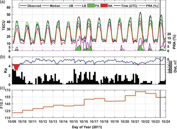
In order to define ionospheric activity over the epicentre, vTEC data were obtained from CODE-GIM with a two-hour time interval. Figure 2(a) shows temporal variations of GIM-vTEC values over the epicentre and Figures 2(b), (c) and (d) show Kp, Dst and F10·7 indices between on 9 October 2011, and 23 October 2011, from 15 days before the Van earthquake. In Figure 2(a), disturbances were detected using the quartile-based running median process. It is expected that the anomalies to be formed in the ionosphere due to earthquakes will last longer than six hours. Therefore, the disturbances longer than six hours are also shown in Figure 2(a) in order to separate the effect of the short-time ionospheric anomalies from vTEC variation. Figure 2(a) depicts a 2–8 TECU increase that is longer than six hours at the epicentre on 9 October, 15–16 October, and 21–23 October within 15 days, 8–9 days and 1–3 days prior the earthquake and no negative change of TEC values were observed 15 days before the Van earthquake. In the analysis of Figures 2(b) and 2(c), it can be seen that the Kp values are below 4, Dst values are between −20 and +20 nT, except for on 9 October (mild geomagnetic activity almost all day) and on 21 October (minor geomagnetic activity over a short period). Figure 2(d) shows that F10·7 values continue to be moderate to high during the 15 days before the earthquake. It reached a maximum value of 166·3 sfu on 21 October 2011.
GIM-vTEC variation of the epicentre, Kp, Dst and F10·7 indices in the 15 pre-earthquake days in which the vertical black line shows the time of Van earthquake. a) GIM-vTEC variation of epicentre calculated from Equation (1). b) Kp, Dst indices and c) F10·7 index. The green bars show positive anomalies and the purple line shows the percentage relative anomaly in (a), the red areas indicate a mild geomagnetic activity according to the Dst index in (b).

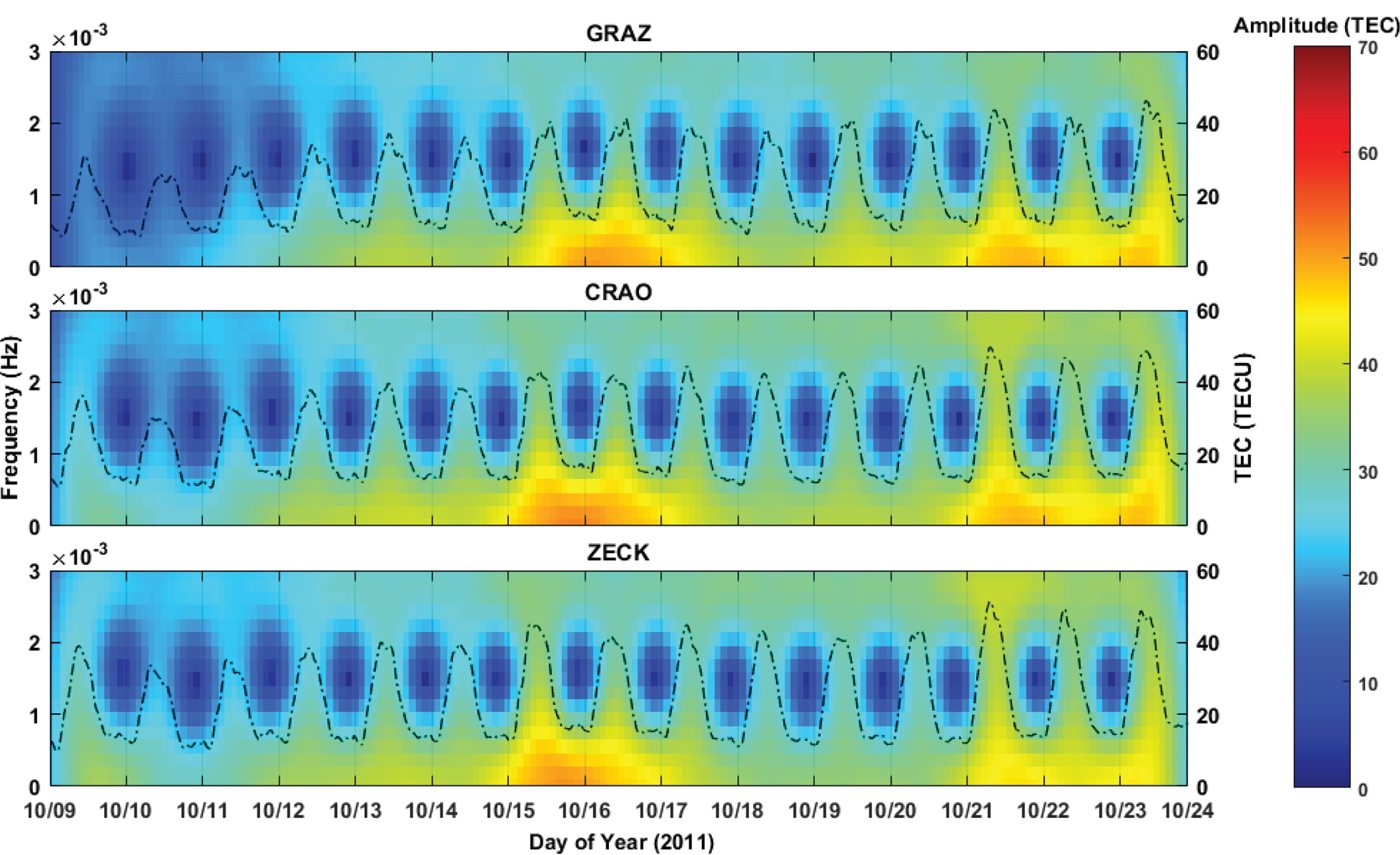
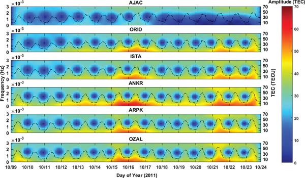
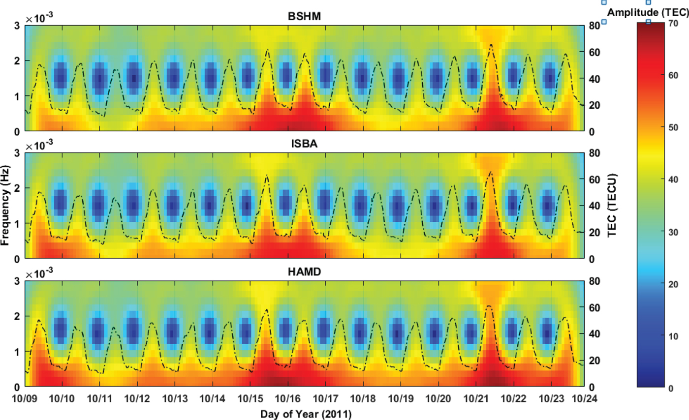
Besides the statistical analyses that were performed concurrently, spectral analyses were carried out to reveal pre-earthquake ionospheric anomalies. In this context, STFT was applied to determine the TEC anomalies both in the time and frequency domains. For the analysis, the sampling rate is taken to be 30 seconds. The results of the STFT analysis are shown in Figures 3–5. In all the figures, the ranges of amplitude are selected from 0 to 70 TECU to crosscheck the STFT results for different areas (for area I–II and III). Figures 3–5 clearly show that high amplitude values of the TEC variation were detected on the days of anomalies identified in the temporal analysis.
STFT analysis of stations in area-I.

STFT analysis of stations in area-II.

STFT analysis of stations in area-III.

In Figure 3, temporal and spectral TEC variation of GRAZ, CRAO and ZECK stations, which are located at area-I are shown. Area-I is located between latitudes 44° N and 47°N to the north of the epicentre. At the GRAZ station, high amplitude values are seen in the afternoon on 15 October, all day on 16 October and 21 October, at sunrise on 17 October and 22 October and from sunrise to afternoon on 23 October. At the CRAO station, high amplitudes were seen all day on 15–16 October and 21 October, at sunrise on 22 October and at sunrise to afternoon on 23 October. At the ZECK station, high amplitudes are seen all day on 15 October, at sunrise to noon on 16 October and at noon to the night on 21 October (lower amplitude than other days). The largest variations of the TEC anomalies correspond to smaller frequencies (≤ 1 × 10⁻³ Hz) and the maximum amplitude is ~50 TECU for all stations in area-I.
In Figure 4, temporal and spectral TEC variation of AJAC, ORID, ISTA, ANKR, ARPK and OZAL stations, which are located in area-II are shown. Area-II was located between 38 · 5° N and 42°N latitudes, approximately at the latitude of the epicentre. At the AJAC station, located at the western of area-II; any high amplitude values relative to other stations are not seen. The maximum amplitude of the station is ~30 TECU on 16 October. At the ORID station, high amplitude values are seen in the afternoon on 15 October, all day on 16 and 21 October, from sunrise to afternoon on 17 and 23 October, from sunrise to noon and sunset to night on 22 October. At the ISTA station, high amplitude values are seen all day on 15–16 October and 21–22 October, at sunrise on 17 October and from sunrise to sunset on October 23. The maximum amplitudes of these two stations are ~52–54 TECU. At the ANKR station, high amplitude values at 55–60 TECU are seen all day on 15–16 October and 21–22 October, from sunrise to noon on 17 October and from sunrise to sunset on October 23. The maximum amplitude was shown at ANKR station in area-II. At the TNPGN-Active stations ARPK and OZAL, located nearest to the epicentre, high amplitude values are seen all day on 15–16 October and 21 October, at sunrise on 17 October and from sunrise to noon on 23 October. The maximum amplitudes of these two stations are ~52–55 TECU. The largest variations of the TEC anomalies correspond to smaller frequencies (≤ 1 × 10⁻³ Hz) for all stations in area-II.
In Figure 5, temporal and spectral TEC variation at BSHM, ISBA, HAMD stations, which are located at area-III, are shown. Area-III is located between latitudes 32 · 5° N and 35° N to the south of the epicentre. This area is also very close to the top of the low-latitude and the Equatorial Ionospheric Anomaly (EIA) region, and therefore the daily TEC values are higher than for areas I and II. At the BSHM station, high amplitude values of 55–65 TECU are seen at sunset on 14 October 14, all day on 15–16 October and 21 October, at sunrise on 17 October and from sunrise to afternoon on 22 October. Only on 11 October was the maximum amplitude lower than 40 TECU at this station. At the ISBA station, high amplitude values of 55–63 TECU are seen from noon to night on 9 October, at sunrise on 10 October, all day on 15–16 October and 21 October, and at sunrise on 22 October. At the HAMD station, high amplitude values of 55–68 TECU were seen in the afternoon on 9 October, at sunrise on 10 October, in the afternoon on 14 October, all day on 15–16 October and 21–22 October, at sunrise on 17 October, and from sunrise to afternoon on 23 October. The largest variations of the TEC anomalies correspond to lower frequencies (≤ 2 × 10⁻³ Hz) for all stations in area-III.
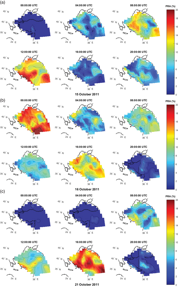
Figures 6(a), (b) and (c) show regional anomaly maps calculated by the quartile-based running median process similar to Figure 2(a). The maps present PRA values bounded by 32°–47° N and 20°–49° E with a four-hour time interval on 15, 16 and 21 October. The PRA values range from 0% to 20%. Natural neighbour interpolation was used to create regional maps and we did not use any extrapolation data. The map grid is 1° × 1°. The RIMs show that there are some local anomaly regions located near the epicentre. The investigated days included high solar activity level and space-weather conditions which affect the ionosphere globally. In this context, the local changes defined in Figure 6 strengthen the idea that there may be some changes related to the Van earthquake in the ionosphere. In particular, when the solar penetration of the ionosphere reduces in the night time, the local changes would be a proof for the presence of earthquake-related anomalies in a period before the earthquake. According to this assumption, the first (00:00 UTC) and last (20:00 UTC) maps in Figures6(a), 6(b) and 6(c) are important indicators. In Figure 6(a), a local anomaly region was detected in the west side of the epicentre of approximately 6% PRA at 00:00 UTC and some local anomaly regions were detected in the west side and northwest side of the epicentre of approximately 12% PRA at 20:00 UTC. In Figure 6(b), there are high PRA values all over Turkey, but particularly those readings to the southwest side of the epicentre are quite remarkable at 00:00 UTC. It can be assumed that these disturbances at night time are related to the Van earthquake. In addition, some local anomaly regions were detected in the west and south side of the epicentre approximately 7% PRA at 20:00 UTC. In Figure 6(c), a remarkable anomaly region was detected at the west side of the epicentre of approximately 9% PRA at 20:00 UTC. The distribution of the anomaly regions in the daytime varies considerably with time and place. For this reason, other data sets such as Outgoing Longwave Radiation (OLR) data may be valuable to research the local changes near the epicentre under high solar activity levels.
Regional ionosphere maps on 15 October (a), 16 October (b) and 21 October (c).

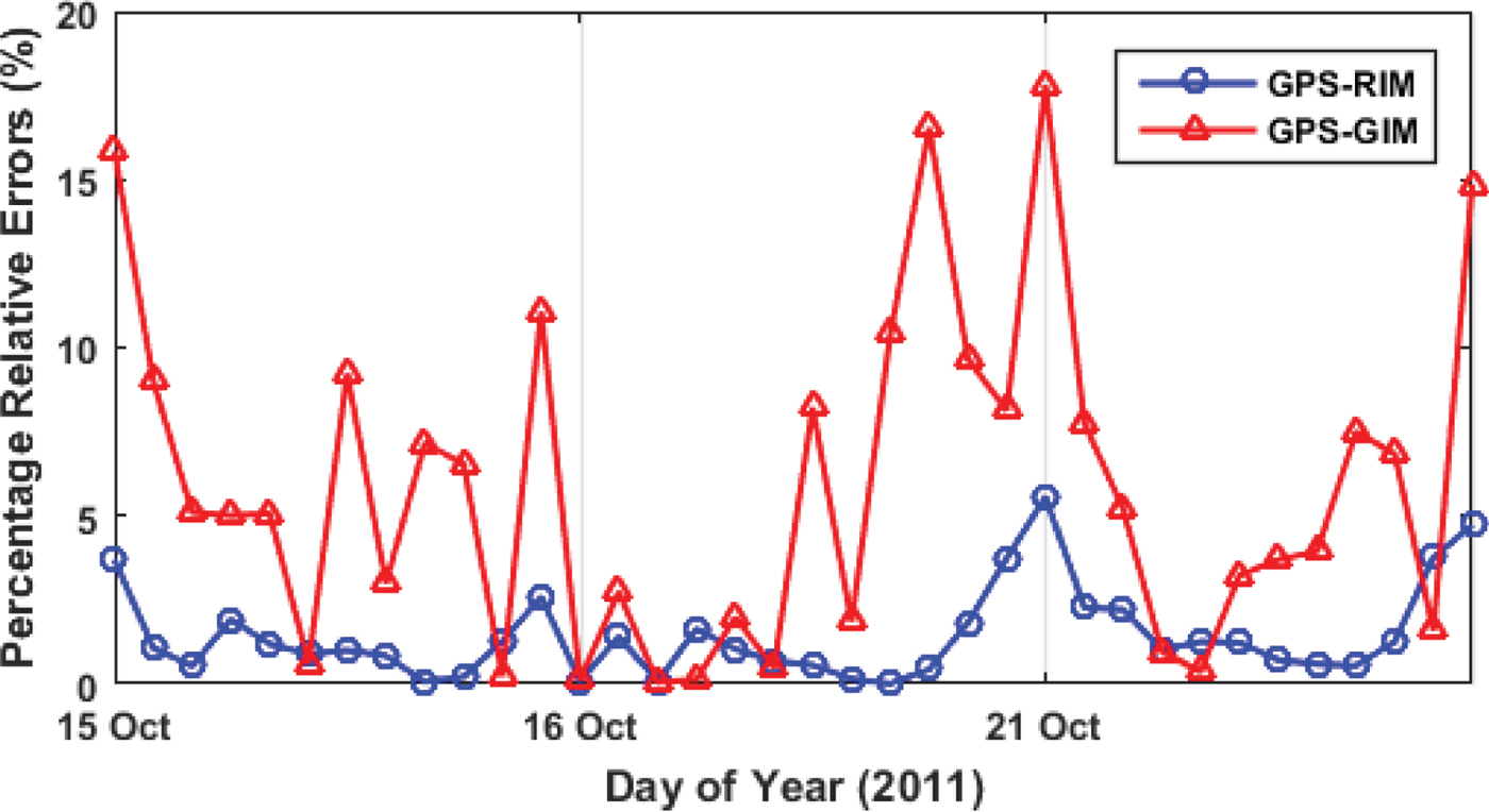
In Figure 7, RIM results are compared with GPS-TEC and CODE-GIM at the location of ANKR station with a two-hour time resolution. Equations (1)–(3) were used to obtain vTEC data at the ANKR station from RIM and GIM. The GPS-TEC data of the ANKR station was calculated using Equations (4)–(11). Figure 7 indicates that RIM results show good agreement with GPS-TEC, which can be accepted as having more precise vTEC values according to GIM-vTEC and it may be used as a reference value to detect ionospheric anomalies. The percentage of relative errors ranges from 0·01–5·56% between GPS-TEC and RIM and 0·06–17·81% between GPS-TEC and CODE-GIM.
The percentage of relative errors between GPS-TEC, RIM, and GIM on October 15, 16 and 21.

4. DISCUSSION AND CONCLUSION
In this study, TEC variation of 11 available IGS stations, 17 TNPGN-Active stations and vTEC variation of the CODE-GIM were analysed using a quartile-based running median process and STFT. RIMs were generated using nine IGS and 17 TNPGN-Active stations by natural neighbour interpolation. RIM results were compared with GPS-TEC and GIM-vTEC. It should be noted that the local TEC values obtained from the GNSS stations are much more precise and distinctive than the global models. The temporal and spectral results show that TEC values have substantial positive variations on 9 October, 15–16 October and 21–23 October, 15 days, 8–9 days and 1–3 days before the earthquake. Regional anomaly maps were generated to investigate the spatial distribution of anomalies. Remarkably, local anomaly regions that were thought to be caused by the Van earthquakes were detected in the night time periods. However, the daytime anomalies were rather scattered and it was also difficult to establish their connection with the earthquake due to the high solar activity. A sudden upsurge of F10·7 on 15–16 October and 20–22 October could be considered as a cause of these anomalies. In addition, most anomaly regions have no distinctive characteristics and are quite variable according to time and place. Therefore, it is not appropriate to reach a conclusion on the cause of TEC anomalies such as their being a precursor to an earthquake or solar activity without further analysis of day time data.
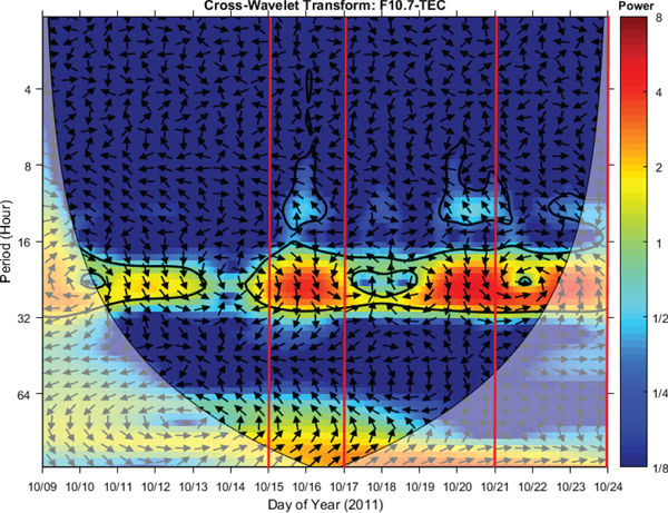
In order to examine the relationship between the ionospheric disturbances and the pre-earthquake solar-terrestrial environment, we used the cross wavelet transform in time-frequency space between values of F10·7 and TEC. In Figure 8, only the result of the OZAL station, which is the nearest station to the epicentre, is presented while the results of other stations have a similar pattern. The CWT shows regions with a high common power and further reveals information about the phase relationship (Grinsted et al., Reference Grinsted, Moore and Jevrejeva2004). Detailed information of the CWT method is given in Section 2.3.4. In Figure 8, thick contours show a 95% significance level against red noise and arrows show the relative phase relationship. When the power of the cross wavelet has passed the significance test, a thick contour occurs and the correlation level between two time series is identified from brighter (low correlation) to more intense (high correlation) colours. As can be seen in Figure 8, there is a correlation between the F10·7 index and TEC values in the abnormal days before the Van earthquake. This means that the TEC may be affected by solar activity on 15–16 October and 21–23 October. The fact that the anomalies on 9 October were caused by a magnetic storm has already been mentioned in earlier parts of this study. Consequently, it is difficult to comment on the ionospheric changes caused by the Van earthquake due to the disturbed space-weather conditions on the abnormal days. A multidisciplinary approach (geophysical, geological, atmospheric, etc) would be useful to identify ionospheric changes as an earthquake precursor under the disturbed space-weather conditions. Some previous studies have mentioned both space weather and earthquake effect in the ionosphere (Yao et al., Reference Yao, Chen, Wu, Zhang and Peng2012; Le et al., Reference Le, Liu, Liu, Zhao, Chen and Wan2013).
WT analysis between the F10·7 index and TEC.

The pre-seismic and co-seismic ionospheric conditions of the Van earthquake have already been investigated by many researchers (Arikan et al., Reference Arikan, Deviren, Lenk, Sezen and Arikan2012; Zolotov et al., Reference Zolotov, Namgaladze and Prokhotov2012; Roland et al., Reference Roland, Vergnolle, Nocquet, Sladen, Dessa, Tavakoli, Nankali and Cappa2013; Alcay, Reference Alcay2016). However, in some of these studies, the solar activity indices have not been considered (Arikan et al., Reference Arikan, Deviren, Lenk, Sezen and Arikan2012; Zolotov et al., Reference Zolotov, Namgaladze and Prokhotov2012). Solar activity was considered in Alcay (Reference Alcay2016) by using the F10·7 and the high level of the F10·7 index (168 sfu) was noticed two days before the earthquake. However, the abnormal days detected in Alcay's study do not coincide with our study as the anomalies were detected in a different region (20°–36° latitude and 80°–100° longitude) by using PPP-based regional Δ TEC maps.
This study shows that temporal, spatial and spectral analyses can be performed successfully together to investigate ionospheric anomalies before a severe earthquake. In particular, in the time-frequency domain, the results were very promising for ionospheric and seismo-ionospheric studies. Thus, the spectral methods could be a useful tool and can be utilised in further studies. STFT can be evaluated as a successful method for detecting ionospheric anomalies and it is also compatible with classical methods. Moreover, STFT is a powerful tool for processing a time series without any background values (mean, median, quite days, etc), so it could be used for other study areas such as navigation, geophysics, geology and climatology. The background values are affected by various atmospheric phenomena but these effects are generally different from the analysed time interval. Since the STFT does not need any comparison (background) value, it provides results that are more reliable. This study also demonstrated that further examinations and analyses have to be realised before any disturbance in the ionosphere evaluated as a precursor of an earthquake. Especially when the space-weather conditions are disturbed, it is inconvenient to establish the relationship between earthquakes and the anomalies obtained by the classical methods. We have confirmed that STFT and CWT are two effective analysis methods that can be used seismo-ionospheric studies.