1 Introduction
Vortical perturbation can be sheltered under a stable shear flow (Hunt & Durbin Reference Hunt and Durbin1999). The shear flow decorrelates the vortices and reduces their convective transport by building a so-called flow-shear-induced transport barrier (Terry Reference Terry2000b ). In a high-shear region with this boundary ‘barrier’, the vortices are isolated and cannot expand beyond this barrier. This phenomenon impacts on the performance of toroidal plasmas (e.g. tokamak and stellarator) (Dritschel Reference Dritschel1989; Beyer et al. Reference Beyer, Benkadda, Fuhr-Chaudier, Garbet, Ghendrih and Sarazin2005; Strugarek et al. Reference Strugarek, Sarazin, Zarzoso, Abiteboul, Brun, Cartier-Michaud, Dif-Pradalier, Garbet, Ghendrih, Grandgirard, Latu, Passeron and Thomine2013), because it enhances plasma confinement and helps to control turbulence and the corresponding convective transport. With both practical and scientific importance, the observation of this shear sheltering has been characterized in highly controlled non-ionized flow experiments (Terry Reference Terry2000a ,Reference Terry b ). However, even though theoretical analysis has estimated that the effect can occur in all types of perturbations and flow regimes (e.g. large or small, unsteady or steady) (Hunt & Durbin Reference Hunt and Durbin1999), shear sheltering has not yet found engineering applications outside ionized plasma fluids. For non-ionized hydrodynamic flows, it has been only observed in non-controllable natural phenomena such as jet or plume-like shear flows and large-scale turbulence in atmospheric boundary layer flows (Hunt & Durbin Reference Hunt and Durbin1999; Terry Reference Terry2000a ,Reference Terry b ). Shats et al. (Reference Shats, Xia, Punzmann and Falkovich2007) reconstructed the effect by generating two-dimensionally confined turbulence in a shallow fluid layer, but it remained in a rather electromagnetically driven flow without relevance in practical hydrodynamic systems. This difficult identification is due to three necessary conditions for the effect, which are hard to meet in non-ionized hydrodynamics: (i) stable shear flow, (ii) long-lasting vortical perturbation in a flow-shear domain and (iii) two-dimensional flow (Terry Reference Terry2000a ,Reference Terry b ).
1.1 Ion concentration polarization and electroconvection
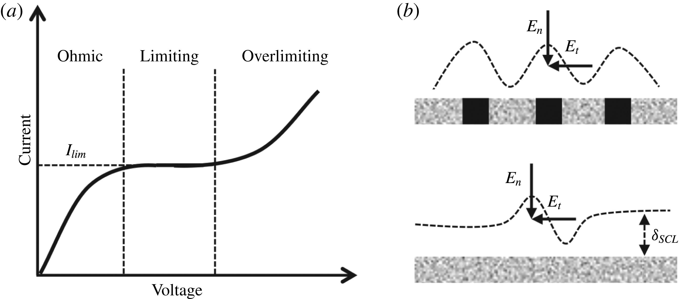
Similarly to electromagnetically induced vortical perturbations in plasmas, ion concentration polarization (ICP) can induce vortical perturbations electrokinetically in electrochemical systems (Probstein Reference Probstein2003; Schoch, Han & Renaud Reference Schoch, Han and Renaud2008). The ICP phenomenon indicates a dynamic shift in ion concentration, where a cation or an anion is selectively transported through ion exchange membranes; cation exchange membranes (CEMs) conduct only cations, and anion exchange membranes conduct only anions. Such a biased ion transport induces unbalanced ion concentrations across the membrane, resulting in depletion of the ions on one side of the membrane and enrichment of the ions on the other side. When the applied voltage is relatively low, the concentration profiles are linear in the depletion and enrichment zones by a combination of diffusion and electromigration. The slope of the concentration profile, which also indicates the amount of ion flux through the membrane, becomes steeper as the voltage is ramped up (Ohmic regime, figure 1
a). At the end, in the depletion zone, the ion concentration reaches zero on the membrane. The current or ion flux is then saturated after this voltage, and the saturated current is known as the limiting current
 $I_{lim}$
(limiting regime, figure 1
a). In the Ohmic and limiting regimes, the linear depletion zone has three layers, an electric double layer, a diffusion layer and a bulk layer, in sequence on the ion exchange membrane (figure 3a in Kwak et al.
Reference Kwak, Guan, Peng and Han2013a
). The electric double layer is the regime where there are more positive (negative) ions than negative (positive) ions on the negatively (positively) charged membrane to satisfy electroneutrality (Probstein Reference Probstein2003). We also call this layer a space charge layer with non-zero space charge
 $\unicode[STIX]{x1D70C}_{e}$
. This layer is generally very thin (a few nanometres), uniform and stable.
On the other hand, under a higher voltage, the strong depletion of co-ions generates an inhomogeneous space charge layer on the membrane, resulting in vortical flows (i.e. electroconvection (EC)) (overlimiting regime, figure 1 a) (Rubinstein & Zaltzman Reference Rubinstein and Zaltzman2000; Kim et al. Reference Kim, Wang, Lee, Jang and Han2007; Rubinstein et al. Reference Rubinstein, Manukyan, Staicu, Rubinstein, Zaltzman, Lammertink, Mugele and Wessling2008). In the seminal work of Rubinstein & Shtilman (Reference Rubinstein and Shtilman1979), the solution of the Poisson–Nernst–Plank equations was obtained in the overlimiting regime. They found that the concentration of counter-ions has non-zero values, whereas the co-ion concentration does tend to zero near the membrane. This extended space charge layer is much thicker than the electric double layer, sufficient to receive a substantial electric body force, but still stable in a one-dimensional system. However, in a two-dimensional system, this extended layer can be spatially inhomogeneous in two ways: heterogeneity of the membrane (Dukhin–Mishchuk model (Dukhin Reference Dukhin1991; Mishchuk & Takhistov Reference Mishchuk and Takhistov1995; Mishchuk, Gonzalez-Caballero & Takhistov Reference Mishchuk, Gonzalez-Caballero and Takhistov2001), figure 1b) and hydrodynamic instability (Rubinstein–Zaltzman model (Rubinstein & Zaltzman Reference Rubinstein and Zaltzman2000; Rubinstein et al. Reference Rubinstein, Manukyan, Staicu, Rubinstein, Zaltzman, Lammertink, Mugele and Wessling2008), figure 1c). The former induces the inhomogeneity of the extended space charge layer, for example, by heterogeneous conducting/non-conducting sites on the membrane. Even if we have a homogeneous membrane, in the latter case, a velocity or concentration fluctuation leads to the inhomogeneous extended space charge layer at sufficiently high voltages. All of these models yield the electric field in the tangential direction to the membrane, and the corresponding electric body force generates vortical fluid flows. This electroconvection vortices mix the solution and transfer additional ions convectively, resulting in a flat concentration profile (with extremely low concentration) and an overlimiting current beyond the diffusion limit.
(a) The current–voltage curve of an ion exchange membrane. (b,c) The two mechanisms for initiating inhomogeneous electric body forces and EC: (b) a heterogeneous membrane with non-conducting sites (black) and (c) a fluctuation of velocity or ion concentration on a homogeneous membrane. Both of these mechanisms induce the inhomogeneous extended space charge layer (
 $\unicode[STIX]{x1D6FF}_{SCL}$
) and the tangential electric field (
 $E_{t}$
) that drives vortical fluid motion. The normal component of the electric field (
 $E_{n}$
) is used to generate the extended space charge layer.

In these mathematical models, the EC has stable symmetric vortex pairs without external fluid flows (non-sheared conditions), and Kim et al. (Reference Kim, Wang, Lee, Jang and Han2007) and Rubinstein et al. (Reference Rubinstein, Manukyan, Staicu, Rubinstein, Zaltzman, Lammertink, Mugele and Wessling2008) directly visualized this symmetric EC. They confirmed that the size of the non-sheared EC is linearly proportional to the voltage, and its speed follows the square of the voltage. Indeed, the degree of the EC strength can be presented by the electric Peclet number,
 $Pe_{E}=\unicode[STIX]{x1D716}{\unicode[STIX]{x1D719}_{0}}^{2}/\unicode[STIX]{x1D707}D$
, where
 $\unicode[STIX]{x1D716}$
is the electric permittivity,
 $\unicode[STIX]{x1D719}_{0}$
is the thermal voltage (
 $=25.85$
mV),
 $\unicode[STIX]{x1D707}$
is the dynamic viscosity of the fluid and
 $D$
is the ion diffusivity. This electric Peclet number can be modified as a more general form, i.e. the electric Rayleigh number
 $Ra_{E}=\unicode[STIX]{x1D716}E^{2}l_{0}^{2}/\unicode[STIX]{x1D707}D$
(where
 $E$
is the electric field and
 $l_{0}$
is the characteristic length). With various monovalent and divalent cations, Choi, Lee & Moon (Reference Choi, Lee and Moon2001) found that the slope of the current–voltage curve in the overlimiting regime increases at a higher
 $Pe_{E}$
. This indicates that a high
 $Pe_{E}$
induces stronger EC vortices which can enhance ion fluxes. In addition, Druzgalski, Andersen & Mani (Reference Druzgalski, Andersen and Mani2013) demonstrated that this stable symmetric EC can be changed to chaotic EC with multi-layer vortex structures in a two-dimensional numerical model.
1.2 Electroconvection under shear flow
Departing from non-sheared EC, sheared EC was recently studied under pressure-driven Hagen–Poiseuille (HP) flow (Kwak, Pham & Han Reference Kwak, Pham, Lim and Han2013b
; Urtenov et al.
Reference Urtenov, Uzdenova, Kovalenko, Nikonenko, Pismenskaya, Vasil’eva, Sistat and Pourcelly2013). Experimental visualization in a miniaturized desalination system and numerical modelling observed the unique characteristics of the EC under shear flow (Kwak et al.
Reference Kwak, Pham, Lim and Han2013b
). In contrast to non-sheared cases, the sheared EC has coherent unidirectional vortices, and these vortices advect along the fluid flow. The direction of vortex rotation is a favourable direction to the fluid flow. In addition, Kwak et al. (Reference Kwak, Pham, Lim and Han2013b
) found that the height of the EC vortex is proportional to
 $V^{2}/U_{HP}$
(where
 $V$
is the voltage and
 $U_{HP}$
is the average flow velocity), instead of a simple linear dependence on
 $V$
. Urtenov et al. (Reference Urtenov, Uzdenova, Kovalenko, Nikonenko, Pismenskaya, Vasil’eva, Sistat and Pourcelly2013) described the initiation of the sheared EC minutely compared with Dukhin–Mishchuk and Rubinstein–Zaltzman models in non-sheared EC. They found that the tangential component of the electric field naturally arises as the ion concentration decreases in the flow-wise direction. This electric field is not strong enough to generate EC vortices. However, it helps to destabilize the extended space charge layer on the homogeneous membrane, and so reduce the threshold voltage to initiate EC. Moreover, the tangential electric field and corresponding body force set the direction towards the inlet, and unidirectional vortices occur. Sheared EC has a different structure and height selection from non-sheared EC, but its strength still has a positive relation to
 $Pe_{E}$
(or
 $Ra_{E}$
). In the overlimiting regime, the high
 $Pe_{E}$
causes a higher slope of the current–voltage curve as well as under shear flow (SI figure 11 in Kwak et al.
Reference Kwak, Pham, Kim, Chen and Han2016).
As described above, EC initiation under shear flow and its superficial characteristics are well documented. However, it is still unknown how the EC vortex interacts with shear flow after its initiation. In this article, we identify two effects of pressure-driven HP flow on sheared EC. One is shear-related and the other is shear-independent. First, we demonstrate that stable EC also transits to chaotic EC under shear flow, and the shear sheltering effect determines when stable or chaotic EC occurs. The microscopic visualization and numerical simulation allow us to capture that the advection of stable EC induces a spatiotemporal vortical perturbation, and chaotic EC occurs when weak shear flow fails to suppress this perturbation, whereas stable unidirectional EC is maintained when strong shear flow shelters the perturbation. By adopting the criterion for shear sheltering, we find the scaling law to bifurcate stable and chaotic EC. It is noted that the electromembrane system we use here is frequently found in hydrodynamic engineering applications (e.g. desalination and fuel cells). The system also clearly departs from the previous
 $E\times B$
flows. Second, beyond the onset of chaotic EC, time-delay phase spaces of attractors and temporal power spectra of current noise illustrate the reduction of chaotic levels under a high flow velocity. The fast mean flow sweeps the vortices on the sidelines of shear sheltering. This vortex sweeping effect dominates only for chaotic EC, whereas it is negligible for the stable EC that exists in the flow-shear-induced transport barrier. Indeed, we confirm that shear sheltering (shear-related) and vortex sweeping (shear-independent) act in different regimes. Lastly, we develop a scaling law to describe the convective ion flux by the sheared EC. The electric Nusselt number shows a power law with the electric Rayleigh number and the Reynolds number, which is reminiscent of the power laws of Rayleigh–Benard convection under shear flow (Grossmann & Lohse Reference Grossmann and Lohse2000; Stevens et al.
Reference Stevens, van der Poel, Grossmann and Lohse2013).
2 Experimental set-up
We utilized an electromembrane desalination cell to visualize EC vortices (Kwak et al.
Reference Kwak, Guan, Peng and Han2013a
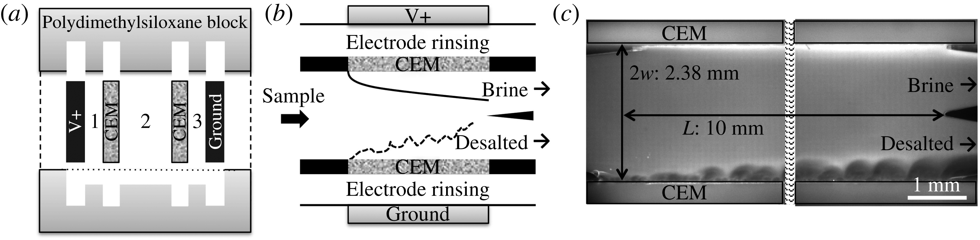
, Reference Kwak, Pham, Kim, Chen and Han2016). After slotting two CEMs and two electrodes between two polydimethylsiloxane blocks, the blocks were bonded together (figure 2
a). Three fluidic channels were then built between the electrodes and the CEMs. The channels between the electrodes and the CEMs were buffer channels (width 1 mm), and the channel between the two CEMs was a sample channel (width
 $2w=2.38$
mm) (figure 2
b,c). The effective channel length (exposed length of the CEMs) was
 $L=10$
mm, and the channel height was
 $h=0.2$
mm. The polydimethylsiloxane blocks were cast from a three-dimensionally printed mould using a Viper si2 SLA system (3D Systems Inc., Rock Hill, SC). FTCM-E (FuMA-Tech GmbH, Germany) and carbon paper (Fuel Cell Store, Inc., Boulder, Co.) were used as the CEMs and the electrodes respectively.
The electromembrane platform and EC under shear flow. (a),(b) Schemes of the cell. (c) Visualized ICP phenomenon at an applied voltage of 20 V and a flow rate of
 $20~\unicode[STIX]{x03BC}\text{L}~\text{min}^{-1}$
.

The desalination cell was then filled with 10 mM NaCl solution with a fluorescent dye (
 $0.78~\unicode[STIX]{x03BC}\text{M}$
Alexa Fluor 488, Invitrogen, Carlsberg, CA). When the dye concentration was low enough, so that these charged dye molecules did not contribute to an electric current, its concentration and the corresponding fluorescent intensity followed the local ion concentrations (Kwak et al.
Reference Kwak, Guan, Peng and Han2013a
). As shown in figure 2(c), under an applied voltage, the ion concentration drop in the desalted flow was visualized as a dark region (lower part of the channel) or the increase of the ion concentration in the brine flow was visualized as a bright region (upper part of the channel). The NaCl solution was loaded by syringe pumps (Harvard Apparatus, PHD 2200) with constant flow rates (
 $2.5{-}20~\unicode[STIX]{x03BC}\text{L}~\text{min}^{-1}$
) between the two CEMs, resulting in parabolic velocity profiles of the pressure-driven HP flows. The corresponding average flow velocity was
 $U_{HP}=0.087{-}0.697~\text{mm}~\text{s}^{-1}$
and the Reynolds number using a hydrodynamic diameter of
 $D_{H}$
(
 $=4wh/(2w+h)=0.369$
mm) was
 $Re_{DH}=0.033{-}0.268$
(
 $Re_{DH}=U_{HP}D_{H}/\unicode[STIX]{x1D708}$
, where
 $\unicode[STIX]{x1D708}$
is the kinematic viscosity of
 $\text{water}=10^{-6}~\text{m}^{2}~\text{s}^{-1}$
). It is noted that these low Reynolds numbers indicate creeping flows where the hydrodynamic instabilities cannot occur inertially. Therefore, the vortices had no chance but to be generated by EC. The velocity profile was three-dimensional with the shallow channel height, but we simply considered it as a two-dimensional flow in the simulation and the theoretical model (figure 3). Between the electrodes and the CEMs (i.e. buffer channels), the same solution flowed with a higher flow rate of
 $50~\unicode[STIX]{x03BC}\text{L}~\text{min}^{-1}$
to rinse products from Faradaic reactions on the electrodes. Under the constant fluid flows, we applied various voltages (0–40 V) to generate the ICP phenomenon on the CEMs, and measured the current responses with a source-measurement unit (Keithley 236, Keithley Instruments Inc., Cleveland, OH). Simultaneously, on an inverted epifluorescence microscope (Olympus IX-71), fluorescent images in the cell were recorded with a thermoelectrically cooled charge-coupled device camera (Hamamatsu Co., Japan). These images were then analysed in ImageJ (NIH, Bethesda, MD) and MATLAB (The MathWorks, Inc., Natick, MA).
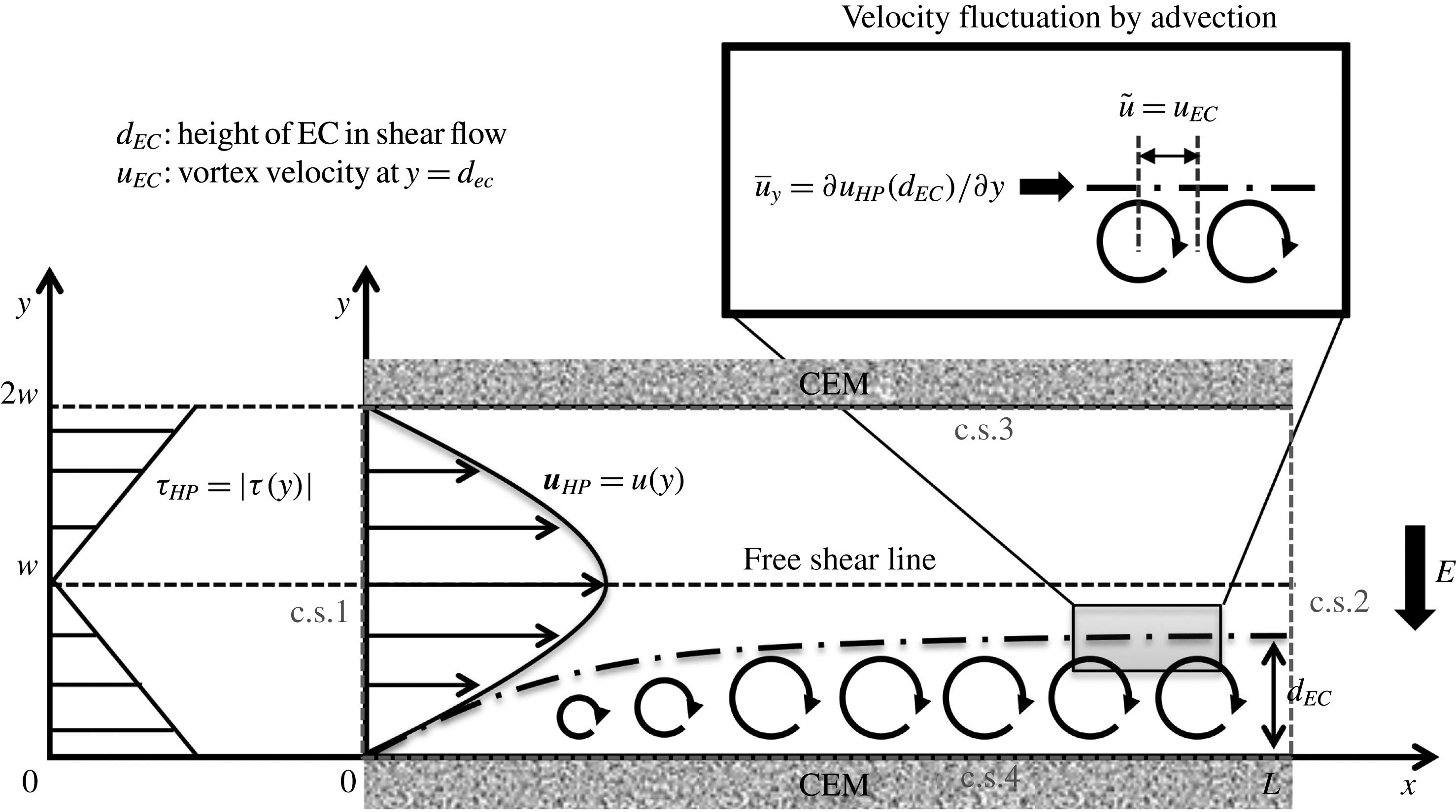
Scheme of the HP flow (
 $\boldsymbol{u}_{HP}$
), corresponding flow shear (
 $\unicode[STIX]{x1D70F}_{HP}$
) and stable unidirectional vortices (circular arrows) in the ion depletion zone (dash-dotted line). Free shear occurs at the middle of the channel
 $(y=w)$
. Electroconvection vortices are assumed to be fully evolved, and have the constant vortex height
 $d_{EC}$
.

3 Computational model
To observe EC dynamics more microscopically, we also considered a simulation model. In this section, we provide a brief description of the governing equations, simulation parameters and boundary conditions. The simulation was carried out using an in-house code, which solved the system of Poisson–Nernst–Planck and Navier–Stokes equations on a two-dimensional domain. The finite volume method was used to discretize the equations. Nonlinearity of the equations was treated directly by using Newton’s method, and the discretized linear systems were solved using the generalized minimal residual method. The equations were solved iteratively until convergence was reached for all variables (the time step was
 $10^{-5}$
s). Details about the simulation method were presented in Pham et al. (Reference Pham, Li, Lim, White and Han2012) and Kwak et al. (Reference Kwak, Pham, Lim and Han2013b
). Between the CEMs in figure 3, the ion transport, electric fields and fluid motions are governed by the Nernst–Planck equations (3.1) and (3.2), Poisson’s equation (3.3) and the Navier–Stokes equations (3.4) and (3.5) respectively:
 $$\begin{eqnarray}\displaystyle & \displaystyle \frac{\unicode[STIX]{x2202}C_{\pm }}{\unicode[STIX]{x2202}t}=-\unicode[STIX]{x1D735}\boldsymbol{\cdot }\boldsymbol{J}_{\pm }, & \displaystyle\end{eqnarray}$$
 $$\begin{eqnarray}\displaystyle & \displaystyle \boldsymbol{J}_{\pm }=-Fz_{\pm }D_{\pm }\unicode[STIX]{x1D735}C_{\pm }-\frac{F^{2}}{RT}z_{\pm }^{2}C_{\pm }D_{\pm }\unicode[STIX]{x1D735}\unicode[STIX]{x1D719}+Fz_{\pm }C_{\pm }\boldsymbol{u}, & \displaystyle\end{eqnarray}$$
 $$\begin{eqnarray}\displaystyle & \displaystyle F(z_{+}C_{+}+z_{-}C_{-})=\unicode[STIX]{x1D70C}_{e}=-\unicode[STIX]{x1D735}\boldsymbol{\cdot }(\unicode[STIX]{x1D716}\unicode[STIX]{x1D735}\unicode[STIX]{x1D719}), & \displaystyle\end{eqnarray}$$
 $$\begin{eqnarray}\displaystyle & \displaystyle \unicode[STIX]{x1D70C}\left(\frac{\unicode[STIX]{x2202}\boldsymbol{u}}{\unicode[STIX]{x2202}t}+\boldsymbol{u}\boldsymbol{\cdot }\unicode[STIX]{x1D735}\boldsymbol{u}\right)=-\unicode[STIX]{x1D735}P+\unicode[STIX]{x1D707}\unicode[STIX]{x1D6FB}^{2}\boldsymbol{u}-\unicode[STIX]{x1D70C}_{e}\unicode[STIX]{x1D735}\unicode[STIX]{x1D719}, & \displaystyle\end{eqnarray}$$
 $$\begin{eqnarray}\displaystyle & \displaystyle \unicode[STIX]{x1D735}\boldsymbol{\cdot }\boldsymbol{u}=0, & \displaystyle\end{eqnarray}$$
where
 $C_{i},J_{i},D_{i}$
and
 $z_{i}$
denote the ion concentration, ion flux, ion diffusivity and ion valence, with subscript
 $i$
for cation (
 $+$
) or anion (
 $-$
). The time
 $t$
, electric potential
 $\unicode[STIX]{x1D719}$
, fluid velocity
 $\boldsymbol{u}$
and space charge
 $\unicode[STIX]{x1D70C}_{e}$
are also defined in the equations. The constants and the parameters are the Faraday constant
 $F$
, gas constant
 $R$
, electric permittivity
 $\unicode[STIX]{x1D716}$
, temperature
 $T$
, fluid dynamic viscosity
 $\unicode[STIX]{x1D707}$
and fluid density
 $\unicode[STIX]{x1D70C}$
. For the simulation model, these governing equations are non-dimensionalized by the reference values for the time
 $\unicode[STIX]{x1D70F}_{0}$
, concentration
 $C_{0}$
, thermal voltage
 $\unicode[STIX]{x1D719}_{0}$
(
 $=25.85$
mV), velocity
 $U_{0}$
, pressure
 $P_{0}$
and average diffusivity
 $D_{0}$
:
 $$\begin{eqnarray}\displaystyle \unicode[STIX]{x1D70F}_{0}=\frac{l_{0}^{2}}{D_{0}},\quad C_{0}=C_{bulk},\quad \unicode[STIX]{x1D719}_{0}=\frac{k_{B}T}{z_{\pm }F},\quad U_{0}=\frac{\unicode[STIX]{x1D716}\unicode[STIX]{x1D719}_{0}^{2}}{\unicode[STIX]{x1D707}l_{0}},\quad P_{0}=\frac{\unicode[STIX]{x1D707}U_{0}}{l_{0}},\quad D_{0}=\frac{D_{+}+D_{-}}{2}. & & \displaystyle \nonumber\\ \displaystyle & & \displaystyle\end{eqnarray}$$
Here,
 $l_{0}$
is the characteristic length,
 $C_{bulk}$
is the bulk ion concentration and
 $k_{B}$
is the Boltzmann constant. The reference velocity
 $U_{0}$
is obtained from the Helmholtz–Smoluchowski velocity
 $(=\unicode[STIX]{x1D716}\unicode[STIX]{x1D709}E/\unicode[STIX]{x1D707})$
with the electric field
 $E$
 $(=\unicode[STIX]{x1D719}_{0}/l_{0})$
and the zeta potential
 $\unicode[STIX]{x1D709}=\unicode[STIX]{x1D719}_{0}$
. The cation/anion diffusivity
 $D_{\pm }$
and the space charge
 $\unicode[STIX]{x1D70C}_{e}$
are also normalized by
 $D_{0}$
and
 $C_{0}$
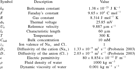
. The values of the constants and parameters used in this simulation model are shown in table 1.
The parameters used in the simulation model.

Then, we solved the local ion concentration, flow velocity and vorticity between the CEMs with proper boundary conditions on the four control surfaces (c.s.1–c.s.4, figure 3). At the inlet (c.s.1), both the cation and anion concentrations
 $C_{\pm }$
were equal to the bulk concentration
 $C_{bulk}$
, and we imposed two-dimensional fluid flow with a parabolic velocity profile and an averaged flow velocity of
 $U_{HP}$
as
 $7.9{-}15.8~\text{mm}~\text{s}^{-1}$
(
 $=800{-}1600U_{0}$
,
 $U_{0}=9.887~\unicode[STIX]{x03BC}\text{m}$
). In addition, the electric field was applied in the
 $y$
-direction only, so the voltage difference across c.s.1 was zero. At the outlet (c.s.2), we assumed that there were no changes of ion concentration, voltage or flow velocity across the control surface. On the CEMs (c.s.3 and c.s.4), it was assumed that the membranes had perfect permselectivities; only cations could transfer to the membrane with zero anion flux. The walls of the CEMs were considered to be impermeable. To generate ICP and EC, a constant voltage difference between the CEMs was applied as the boundary conditions: a constant voltage
 $V$
(
 $=26{-}45\unicode[STIX]{x1D719}_{0}$
,
 $\unicode[STIX]{x1D719}_{0}=25.85~\text{mV}$
) at the upper membrane and zero voltage at the lower membrane. The boundary conditions are summarized as follows:
 $$\begin{eqnarray}\text{c.s.1}:~C_{\pm }=C_{bulk},\quad \frac{\unicode[STIX]{x2202}\unicode[STIX]{x1D719}}{\unicode[STIX]{x2202}n}=0,\quad \boldsymbol{u}=\frac{6U_{HP}y}{2w}\left(1-\frac{y}{2w}\right);\end{eqnarray}$$
 $$\begin{eqnarray}\text{c.s.2}:~\frac{\unicode[STIX]{x2202}C_{\pm }}{\unicode[STIX]{x2202}n}=0,\quad \frac{\unicode[STIX]{x2202}\unicode[STIX]{x1D719}}{\unicode[STIX]{x2202}n}=0,\quad \frac{\unicode[STIX]{x2202}\boldsymbol{u}}{\unicode[STIX]{x2202}n}=0;\end{eqnarray}$$
 $$\begin{eqnarray}\text{c.s.3}:~\boldsymbol{J}_{-}=0,\quad \boldsymbol{u}=0,\quad \unicode[STIX]{x1D719}=V;\end{eqnarray}$$
 $$\begin{eqnarray}\text{c.s.4}:~\boldsymbol{J}_{-}=0,\quad \boldsymbol{u}=0,\quad \unicode[STIX]{x1D719}=0;\end{eqnarray}$$
where
 $\boldsymbol{n}$
is the normal vector of the control surfaces. For both the simulation model and the experiment set-up, we shared the physical properties including fluidic and electric parameters (table 1). However, with a limited computational budget, we scaled down the size of the channel (width
 $60~\unicode[STIX]{x03BC}\text{m}$
, length
 $150~\unicode[STIX]{x03BC}\text{m}$
and unit height 1 m). In this two-dimensional simulation, the local ion concentrations, electric fields and flow velocities varied nonlinearly and rapidly in an extremely thin layer (0.01 % of the channel width) near the membranes. Such nonlinear properties lead the discretized Jacobian of the Poisson–Nernst–Planck equations into an ill-conditioned matrix, which it is difficult to converge to a feasible solution. This problem with EC simulations was also found in previous studies (Rubinstein et al.
Reference Rubinstein, Manukyan, Staicu, Rubinstein, Zaltzman, Lammertink, Mugele and Wessling2008; Pham et al.
Reference Pham, Li, Lim, White and Han2012; Druzgalski et al.
Reference Druzgalski, Andersen and Mani2013), so they also used micrometre-scale models. Although our simulation size was smaller than the experimental one, we adjusted the flow velocity and the applied voltage in the simulation, and obtained the same range of the dimensionless EC height (
 $d_{EC}/w$
) as that in the experiments. This allowed us to match the EC dynamics in the experiments and simulations (Kwak et al.
Reference Kwak, Pham, Lim and Han2013b
).
4 Results and discussion
4.1 Four ICP regimes under shear flow
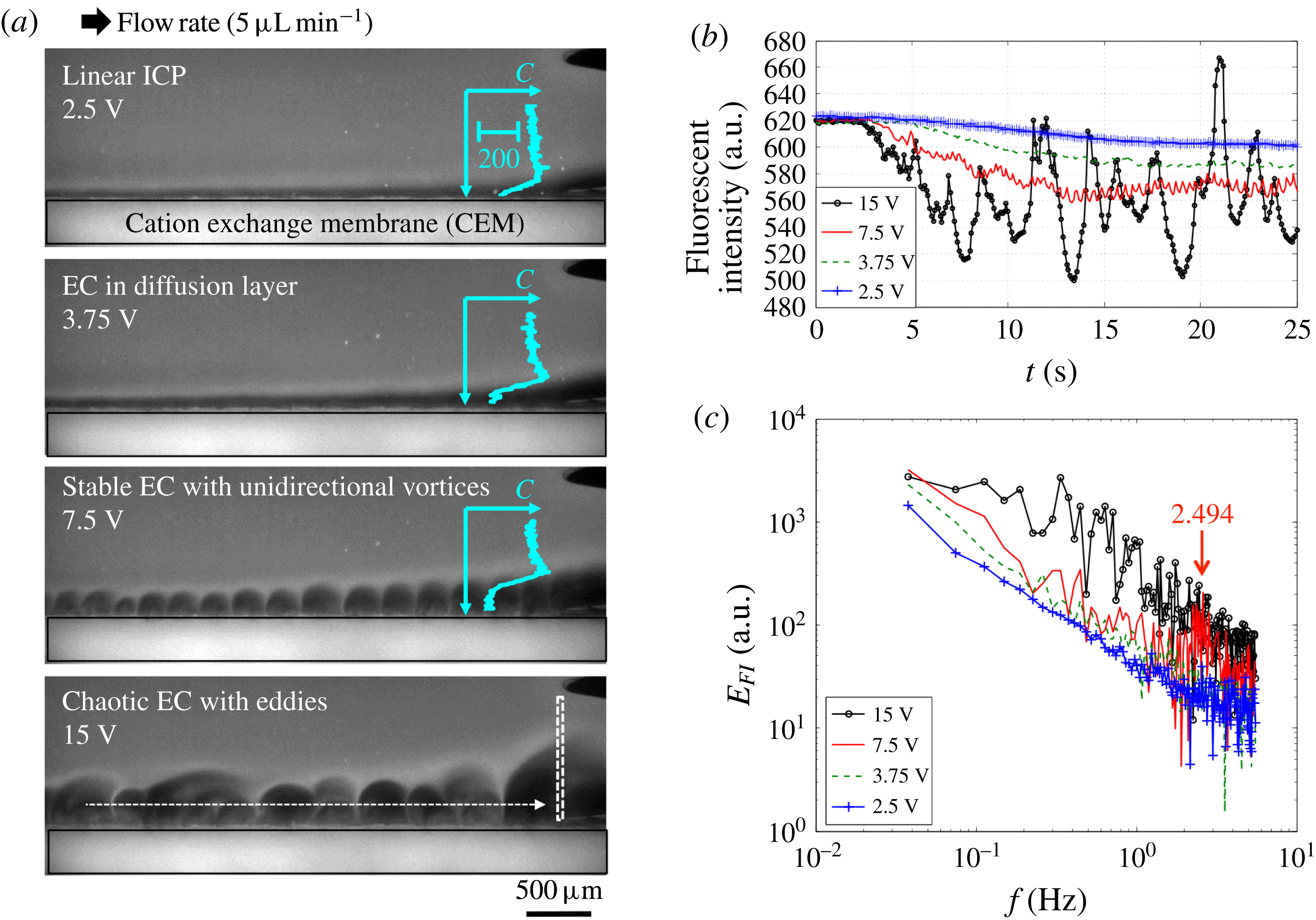
To elucidate the effects of the flow shear on EC, we first differentiate ICP regimes under various flow rates and applied voltages in the experimental platform (figure 4). A qualitative concentration profile by fluorescent imaging shows the four regimes in figure 4(a) (supporting movie 1 at https://doi.org/10.1017/jfm.2016.870): linear ICP with a smooth diffusion layer (2.5 V), EC in the diffusion layer when the vortex size is smaller than diffusion layer thickness (3.75 V), stable EC with unidirectional vortices (7.5 V) and chaotic EC with eddies (15 V). It is noteworthy that previous works recognized only two ICP regimes: linear ICP and EC (Rubinstein & Zaltzman Reference Rubinstein and Zaltzman2000; Kim et al. Reference Kim, Wang, Lee, Jang and Han2007; Rubinstein et al. Reference Rubinstein, Manukyan, Staicu, Rubinstein, Zaltzman, Lammertink, Mugele and Wessling2008; Kwak et al. Reference Kwak, Pham, Lim and Han2013b ).
Four ICP regimes under shear flow. (a) In situ fluorescent imaging identifies four different ICP regimes under shear flow: linear ICP (2.5 V), EC in diffusion layer (3.75 V), stable EC (7.5 V) and chaotic EC (15 V) at a fixed flow rate (
 $5~\unicode[STIX]{x03BC}\text{L}^{-1}~\text{min}^{-1}$
). The images are sectioned to display the ion depletion zones (the back and lower parts (
 $3~\text{mm}\times 1~\text{mm}$
) of the whole channel (figure 2
c)). The inset profiles indicate fluorescent intensity profiles scaled by 200 a.u., which describe the ion concentration
 $C$
qualitatively. (b) Fluorescent intensity profiles at the channel end (white dotted box in (a)). This intensity/concentration drop also indicates the desalting performance (Kwak et al.
Reference Kwak, Guan, Peng and Han2013a
). (c) The power spectra of the intensity fluctuation
 $E_{FI}$
. Fast Fourier transform was applied to the curves of the intensity–time profiles in (b).

When the applied voltage is lower than the critical value for EC (
 ${<}3$
V in this experiment (this will be described in § 4.5)), the ion concentration drops linearly in the ion depletion zone (inset profile at 2.5 V, figure 4
a). As a result, we can observe a smooth diffusive boundary layer along the membrane (dark region along the CEM at 2.5 V, figure 4
a). Such a smooth depletion zone has been well described by the convective-diffusion model (Probstein Reference Probstein2003). Under higher voltages (beyond the critical value for EC), three different regimes are observed with a unique concentration profile, i.e. flat depletion zone and sharp concentration drop at the boundary (inset profiles at 3.75–7.5 V, figure 4
a). When the height of EC is smaller than the thickness of the diffusion layer, we still observe the smooth depletion zone (at 3.75 V, figure 4
a). EC vortices in the diffusion layer slightly perturb the boundary (supporting movie 1). However, when the vortices become dominant, the shapes of the depletion zone are totally changed (at 7.5 V, figure 4
a). As we characterized previously (Kwak et al.
Reference Kwak, Pham, Lim and Han2013b
), stable EC with coherent unidirectional vortices occurs under shear flow.
If the voltage becomes much higher, we observe that this stable EC can be chaotic (at 15 V, figure 4
a); instead of the coherent unidirectional vortices, chaotic eddies with spatiotemporal chaos are observed. This chaotic EC has dynamics reminiscent of inertia-driven turbulence at a high
 $Re$
, but it happens at a low
 $Re$
and at a high
 $Ra_{E}$
. In an electrohydrodynamic system, Posner, Pérez & Santiago (Reference Posner, Pérez and Santiago2012) observed a similar periodic-to-chaotic transition, and confirmed that there is a critical
 $Ra_{E}$
for electrohydrodynamic instability (
 ${\sim}200$
). This
 $Ra_{E}$
considered the conductivity ratio at the interface
 $\unicode[STIX]{x1D6FE}$
as
 $Ra_{E}=(\unicode[STIX]{x1D716}E^{2}h^{2}/D_{eff}\unicode[STIX]{x1D707})((\unicode[STIX]{x1D6FE}-1)/\unicode[STIX]{x1D6FE})$
, where
 $D_{eff}$
is the effective diffusivity (
 $D_{eff}=2D_{+}D_{-}/(D_{+}+D_{-})=1.607\times 10^{-9}~\text{m}^{-2}~\text{s}^{-1}$
for NaCl). According to this definition, in our system, the ion concentration in the depletion zone drops to significantly lower than 1 % of the bulk ion concentration (Kim et al.
Reference Kim, Wang, Lee, Jang and Han2007; Kwak et al.
Reference Kwak, Guan, Peng and Han2013a
). Then,
 $\unicode[STIX]{x1D6FE}$
is approximately 100,
 $(\unicode[STIX]{x1D6FE}-1)/\unicode[STIX]{x1D6FE}\sim 1$
and
 $E\sim V/d_{EC}$
. For example, at
 $V=15$
V and
 $d_{EC}\sim 0.25~\text{mm}$
in figure 4(a),
 $Ra_{E}$
is
 $5.62\times 10^{4}$
; this is considerably over the critical
 $Ra_{E}=200$
for inducing electrohydrodynamic instability.
4.2 Stable-to-chaotic EC transition: shear sheltering
4.2.1 Identifying stable and chaotic EC
Qualitative ion concentration profiles by fluorescent imaging represent four ICP regimes under shear flow. Here, the most unique behaviour of this sheared EC is the transition from stable to chaotic EC. Adopting the concept of shear sheltering, we hypothesize that chaotic EC will occur when the vortical perturbation by stable EC overcomes the shear of the HP flow. In contrast to other neutral-fluid flows in Terry (Reference Terry2000a
), this sheared EC exactly satisfies the three preconditions to realize shear sheltering, because the sources of perturbation (EC) and the flow shear (no-slip wall) are decoupled. In detail, these conditions are as follows. (i) The millimetre-scale device maintains the HP flow in a stable laminar flow regime (
 $Re<1$
). (ii) Under an applied voltage, the EC lasts for a long time in the flow-shear domain. (iii) The high aspect ratio of the channel (width (2.38 mm)/height (0.2 mm)
 $=$
11.9) confines the HP flow and EC vortices in the two-dimensional (
 $x{-}y$
) plane, as shown in figures 3 and 4.
If we follow along the membrane (white arrow in figure 4
a), the diffusion-dominant cases (2.5–3.75 V) show smooth intensity drops with linear ion depletion zones. However, the EC-dominant cases show periodic or random perturbation of the intensity with stable (7.5 V) or chaotic EC (15 V). With the vortex advection in a flow-wise direction, such fluctuations can be gathered by measuring the fluorescent intensity at the channel end (white dotted boxes in figure 4
a) (figure 4
b). When we apply Fast Fourier transform to these intensity–time profiles, stable EC is distinguished with the peak in the power spectrum (figure 4
c). For example, the periodicity of coherent vortices at 7.5 V is well captured with the peak frequency
 $f=2.494$
. The wavelength
 $\unicode[STIX]{x1D706}=220~\unicode[STIX]{x03BC}\text{m}$
calculated from the peak frequency is well matched to the size of the EC vortices (
 $=U_{EC}/f$
, where the advection velocity
 $U_{EC}=0.55~\text{mm}~\text{s}^{-1}$
at 7.5 V, figure 4
a). In contrast, the fluorescent intensity of chaotic EC has strong and broad frequency noise. The power spectra of the intensity fluctuations for the two diffusion-dominant cases (2.5–3.75 V) are
 ${\sim}10$
times smaller than those of the two EC-dominant cases (7.5–15 V). If we distinguish stable and chaotic ECs and place them in the voltage (
 $V$
)–flow rate (
 $Q$
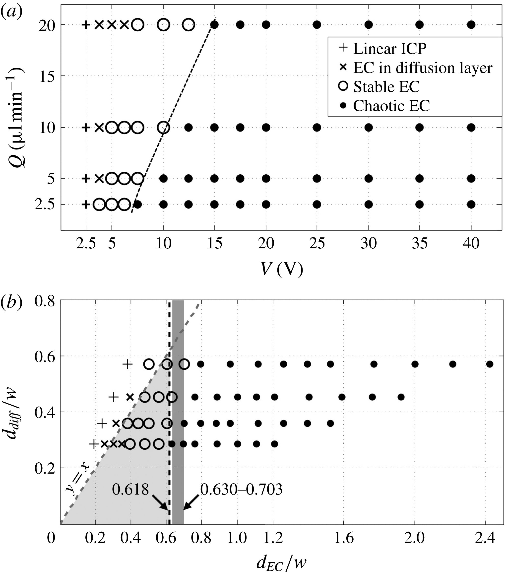
) plane, a delay in transition from stable to chaotic EC is observed under a higher flow rate (with higher shear), in accordance with our hypothesis (dotted line in figure 5
a).
Phase diagrams of the four ICP regimes under shear flow. The experiments were performed under four flow rates (2.5, 5, 10 and
 $20~\unicode[STIX]{x03BC}\text{L}~\text{min}^{-1}$
) and 14 applied voltages (2.5–40 V). Fluorescent images for all of the experiments are available in the supporting information. The results are located in (a) the
 $V$
–
 $Q$
plane and (b) the
 $d_{EC}/w$
–
 $d_{diff}/w$
plane. Here,
 $d_{EC}/w$
is calculated by substituting the applied voltage
 $V$
and the averaged flow velocity
 $U_{HP}$
in
 $d_{EC}/w=0.00963(V^{2}/U_{HP})^{1/3}$
;
 $d_{diff}/w$
is calculated using
 $d_{diff}/w=0.252(U_{HP})^{-1/3}$
. Electroconvection is not observed at 2.5 V; thus, we categorize these cases as linear ICP. The threshold line moves slightly to the right compared with the theoretical value (
 $d_{EC}/w=0.618$
), presumably because we overestimate the voltage drop in the EC zone (
 $V_{EC}$
) by assuming
 $V\sim V_{EC}$
.

4.2.2 Shear sheltering of EC: scaling analysis
To verify that the transition from stable to chaotic EC is governed by the shear sheltering, we adopt the scaling law for the strong-shear limit
 $\unicode[STIX]{x1D716}_{s}<1$
(equation (2.17) in Terry (Reference Terry2000b
)), and designate the threshold of stable and chaotic EC:
 $$\begin{eqnarray}\unicode[STIX]{x1D716}_{s}=\frac{\tilde{u} }{\unicode[STIX]{x1D6FF}y\bar{u}_{y}}<1,\end{eqnarray}$$
where
 $\tilde{u}$
is the eddy velocity (i.e. the magnitude of the velocity perturbation),
 $\unicode[STIX]{x1D6FF}y$
is the region away from the flow shear and
 $\bar{u}_{y}$
is the mean flow shear (
 $=~y$
-differential of the mean flow velocity). Equation (4.1) expresses the ratio between the strengths of vortical perturbation and the flow shear in the velocity dimension. In EC experiments and simulations, the stable EC vortices generate a velocity perturbation. The vortices advect along the membrane, then the velocity is periodically changed at a fixed location on the EC boundary (
 $y=d_{EC}$
) as the valley of the vortex passes or the vortex peak passes (black box, figure 3
c). The magnitude of this velocity change is approximately equal to the EC vortex speed
 $u_{EC}$
. We will quantify this periodic velocity perturbation with stable EC in the simulation (§ 4.6). Here, if the flow shear shelters this perturbation (
 $\unicode[STIX]{x1D716}_{s}<1$
), its momentum remains in the vortices, and stable unidirectional vortices are maintained. In contrast, under weak flow shear (
 $\unicode[STIX]{x1D716}_{s}>1$
), the vortical perturbation spreads out and generates chaotic EC.
From the parabolic velocity profile,
 $\bar{u}_{y}$
is expressed by the average flow velocity
 $U_{HP}$
, channel width
 $2w$
, height
 $h$
and hydrodynamic diameter
 $D_{H}$
:
 $\bar{u}_{y}=64U_{HP}/D_{H}^{2}(w-y)$
. Against this flow shear, the vortical perturbation
 $\tilde{u}$
(
 $=$
EC vortex speed
 $u_{EC}$
) is scaled by the electro-osmotic slip velocity
 $u_{s}$
in the Rubinstein–Zaltzman model (Rubinstein & Zaltzman Reference Rubinstein and Zaltzman2000). We consider that the slip velocity on the membrane is equal to the outermost vortex velocity of the EC,
 $$\begin{eqnarray}u_{EC}=u_{s}=-\frac{\unicode[STIX]{x1D716}V_{EC}^{2}}{32\unicode[STIX]{x03C0}\unicode[STIX]{x1D707}}\frac{\unicode[STIX]{x2202}^{2}C/\unicode[STIX]{x2202}x\unicode[STIX]{x2202}y}{\unicode[STIX]{x2202}c/\unicode[STIX]{x2202}y}|_{y=0}.\end{eqnarray}$$
Here,
 $V_{EC}$
is the voltage drop across the EC vortex. Under stable EC, we assume that (i) the vortex is a hemisphere (the vortex width
 $=$
the vortex
 $\text{height}=d_{EC}$
), (ii) the ion concentration at the vortex core is almost zero and (iii) the ion concentration changes in the vortex only (Rubinstein & Zaltzman Reference Rubinstein and Zaltzman2000; Kwak et al.
Reference Kwak, Pham, Lim and Han2013b
). Then, the ion concentration gradient is approximately
 $\unicode[STIX]{x2202}C/\unicode[STIX]{x2202}x=\unicode[STIX]{x2202}C/\unicode[STIX]{x2202}y\sim C_{bulk}/d_{EC}$
, resulting in
 $$\begin{eqnarray}u_{EC}\sim \frac{\unicode[STIX]{x1D716}V_{EC}^{2}}{\unicode[STIX]{x1D707}}\frac{C_{bulk}/d_{EC}^{2}}{C_{bulk}/d_{EC}}\sim \frac{\unicode[STIX]{x1D716}}{\unicode[STIX]{x1D707}}\frac{V_{EC}^{2}}{d_{EC}}.\end{eqnarray}$$
We note that the Dukhin–Mishchuk model (Mishchuk et al.
Reference Mishchuk, Gonzalez-Caballero and Takhistov2001) also scales the same
 $u_{EC}$
. In this model, the slip velocity
 $u_{s}$
on the surface with the heterogeneous electric double layer is
 $u_{s}\sim \unicode[STIX]{x1D716}aE^{2}/\unicode[STIX]{x1D707}$
, where
 $a$
is a characteristic length representing the heterogeneity of the space charge in the double layer and
 $E$
is the applied electric field across
 $a$
. On the membrane surface with stable EC, space charge heterogeneity follows the ion concentration difference across the EC vortex; the thickness of the electric double layer (i.e. the Debye length) is proportional to the ion concentration
 $C^{1/2}$
(Schoch et al.
Reference Schoch, Han and Renaud2008). Then, the characteristic length
 $a$
is equal to the EC size
 $d_{EC}$
. Under the electric field
 $E\sim V_{EC}/d_{EC}$
, the slip velocity becomes
 $u_{s}\sim (\unicode[STIX]{x1D716}/\unicode[STIX]{x1D707})(V_{EC}^{2}/d_{EC})$
, which is the same result as that from the Rubinstein–Zaltzman model (equation (4.3)). Finally, substituting
 $\tilde{u} =u_{EC},\bar{u}_{y}$
at
 $y=d_{EC}$
, and
 $\unicode[STIX]{x1D6FF}y=w$
(the location with zero flow shear) into the equation (4.1) yields
 $$\begin{eqnarray}\frac{\unicode[STIX]{x1D716}D_{H}^{2}}{64\unicode[STIX]{x1D707}w^{3}}\frac{V_{EC}^{2}}{U_{HP}}<\frac{d_{EC}}{w}\left(1-\frac{d_{EC}}{w}\right).\end{eqnarray}$$
The left-hand side of (4.4) is the same as
 $(d_{EC}/w)^{3}$
according to the scaling law of the dimensionless sheared EC height
 $d_{EC}/w=[(\unicode[STIX]{x1D716}D_{H}^{2}/64\unicode[STIX]{x1D707}w^{3})(V_{EC}^{2}/U_{HP})]^{1/3}$
(Kwak et al.
Reference Kwak, Pham, Lim and Han2013b
; Urtenov et al.
Reference Urtenov, Uzdenova, Kovalenko, Nikonenko, Pismenskaya, Vasil’eva, Sistat and Pourcelly2013). Finally, the strong-shear limit (
 $\unicode[STIX]{x1D716}_{s}<1$
) for sheltering the EC vortical perturbation is represented by a simple quadratic function,
 $$\begin{eqnarray}\displaystyle & \displaystyle \left(\frac{d_{EC}}{w}\right)^{2}+\frac{d_{EC}}{w}-1<0, & \displaystyle\end{eqnarray}$$
 $$\begin{eqnarray}\displaystyle & \displaystyle 0\leqslant \frac{d_{EC}}{w}<0.618, & \displaystyle\end{eqnarray}$$
which is entirely determined by the dimensionless EC height. This is because the
 $y$
-location (the distance from the membrane) determines the strengths of both the EC vortex and the flow shear. According to this criterion, stable EC occurs if
 $d_{EC}/w<0.618$
and chaotic EC occurs if
 $d_{EC}/w>0.618$
.
Figure 5(b) shows the experimental results remapped in the
 $d_{EC}/w$
–
 $d_{diff}/w$
plane, where
 $d_{diff}/w$
is the dimensionless thickness of the diffusion layer:
 $d_{diff}/w=[(D_{eff}/wU_{HP})(L/w)]^{1/3}$
(equation (6.2.12) in Probstein (Reference Probstein2003)). In (4.4), the voltage drop in the EC vortex is approximately equal to the applied voltage (
 $V\sim V_{EC}$
). This is because a large part of the applied voltage drops in the EC zone, which has a extremely low ion concentration (Kwak et al.
Reference Kwak, Pham, Lim and Han2013b
). By summing the EC-dominant condition (
 $d_{EC}/w>d_{diff}/w$
) and the strong-shear limit (
 $d_{EC}/w<0.618$
), we can observe the clear regime for stable EC (dark grey box, figure 5
b). This theoretical regime for stable EC is exactly matched with the experimental result. In the experiment, the threshold for stable and chaotic EC appears at
 $d_{EC}/w=0.630{-}0.703$
(light grey box, figure 5
b). Chaotic EC is observed when
 $d_{EC}/w>0.618$
, and the EC vortex (and its effects) is invisible when
 $d_{EC}/w<d_{diff}/w$
(diffusion-dominant regime).
4.3 Attractors in a time-delay phase space
In the previous section, we described how the periodic-to-chaotic transition of EC is due to shear sheltering. In this section, we draw attractors in a time-delay phase space (Packard et al.
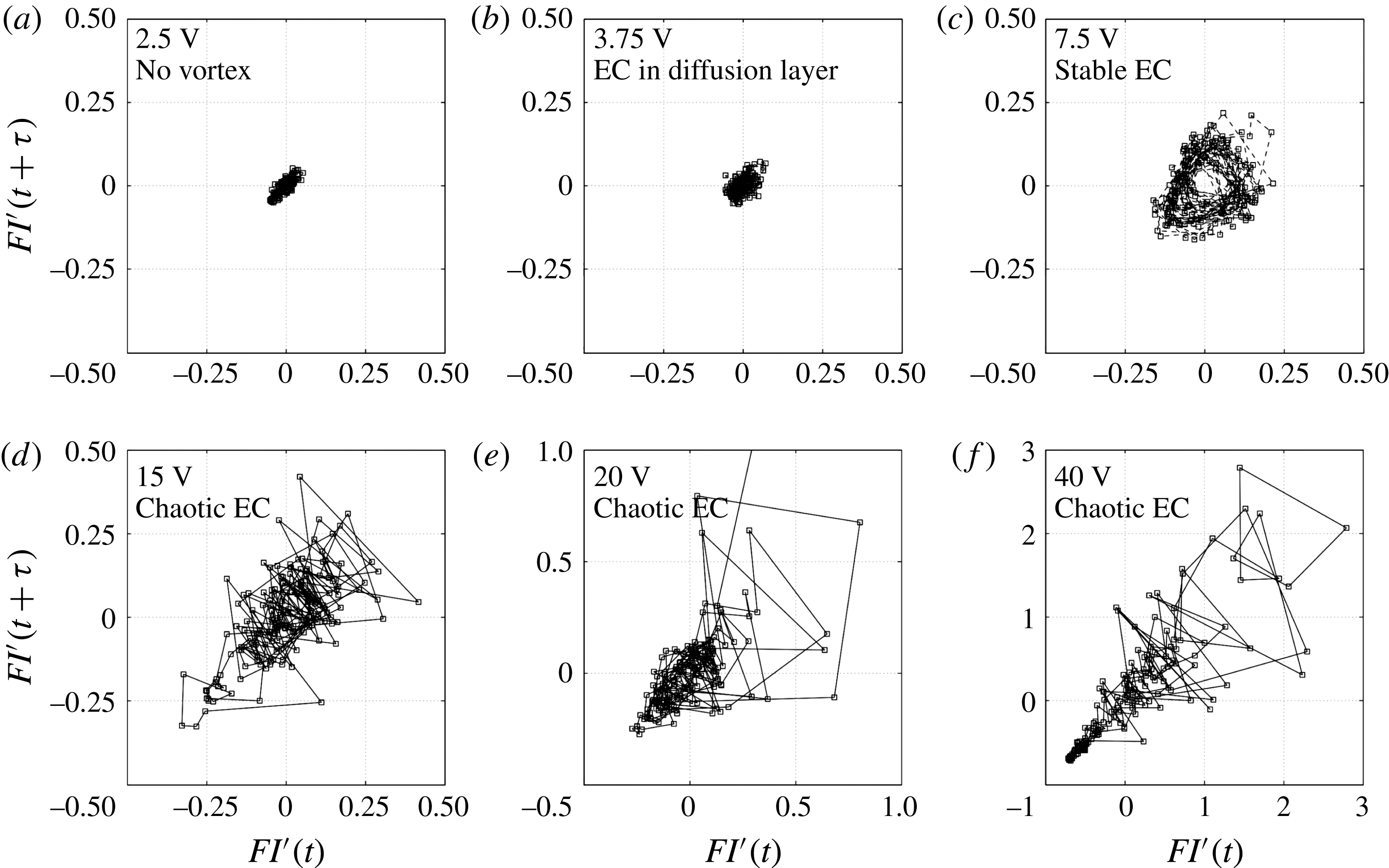
Reference Packard, Crutchfield, Farmer and Shaw1980; Swinney Reference Swinney1983; Cross & Hohenberg Reference Cross and Hohenberg1993) and illustrate the sequence between steady, periodic and chaotic states of the sheared EC precisely (figure 6). At a fixed point on the diffusion or EC boundary layer, we recorded the time series of the fluorescent intensity
 $FI(t)$
. After normalizing the intensity with its average value (
 $FI^{\prime }(t)$
), the phase-space trajectory was mapped by plotting [
 $FI^{\prime }(t),FI^{\prime }(t+\unicode[STIX]{x1D70F})$
], where
 $\unicode[STIX]{x1D70F}$
is the time delay (90 ms). This method has been used to trace various periodic-to-chaotic transitions in hydrodynamic instabilities, e.g. Taylor–Couette flows (Vastano & Moser Reference Vastano and Moser1991; Wulf, Egbers & Rath Reference Wulf, Egbers and Rath1999; Sinha, Kevrekidis & Smits Reference Sinha, Kevrekidis and Smits2006) and electrohydrodynamic instability (Bassett & Hudson Reference Bassett and Hudson1989; Posner et al.
Reference Posner, Pérez and Santiago2012). We are also able to trace the four ICP regimes and corresponding steady–periodic–chaotic transitions with different attractors. At 2.5 V, there is a slow and long wave fluctuation of the smooth boundary layer, probably because of external sources (e.g. pressure variation by the syringe pump) (supporting movie 1). Without sudden changes of the fluorescent intensity, we have a steady attractor with small fluctuations along
 $y=x$
(figure 6
a). As EC in diffusion layer perturbs this boundary layer, a sudden yet small fluctuation is presented in the steady attractor with additional fluctuations along
 $y=-x$
(figure 6
b). Next, stable EC induces a periodic fluctuation of the fluorescent intensity, resulting in a cyclic attractor (figure 6
c). The coherence of the stable vortices is shown as a single cycle of the attractor. The chaotic fluctuation of chaotic EC is represented by the scattered dots (figure 6
d–f).
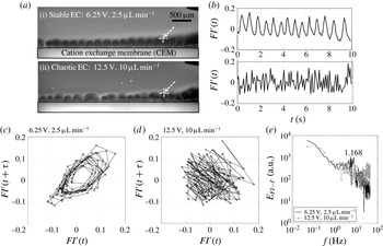
In addition, a dynamic system based on the Navier–Stokes equations usually has subharmonic, quasiperiodic and/or intermittent phases between the periodic and chaotic states (Gollub & Benson Reference Gollub and Benson1980). To check for the existence of these intermediate states, the phase-space trajectories are presented for one stable EC and one chaotic EC at the threshold (
 $d_{EC}/w=0.703$
) (figure 7 and supporting movie 2). The two cases have similar vortex sizes, but the internal structures are totally different. The stable EC at the threshold shows a subharmonic oscillation and an attractor with multiple cycles (figure 7
b,c) (Bassett & Hudson Reference Bassett and Hudson1989; Wulf et al.
Reference Wulf, Egbers and Rath1999; Sinha et al.
Reference Sinha, Kevrekidis and Smits2006). On the other hand, the chaotic EC at the threshold has an attractor with a single group (figure 7
d). As can be seen in figure 7(a), the vortex size varies, but the range of this variation is limited to half of the vortex. Therefore, instead of the fan-shaped scattered attractors in figure 6(d–f), this chaotic attractor just spreads in
 $\mid FI^{\prime }(t)\mid <1$
. This magnitude of the intensity fluctuation is the same as that in the stable EC case. Consequently, the power spectrum of
 $FI(t)$
with chaotic EC loses the peak of stable EC, and obtains high-frequency noise over the peak (
 $f>1.168$
Hz) (figure 7
e). At
 $f<1.168$
Hz, the spectra of stable/chaotic EC are mostly overlapped, because this chaotic EC has fluctuations no larger than the size of the stable EC vortex. A similar trend was also observed in other dynamic systems, and it subdivides the phases into a weak chaotic state (figure 7
d) and a strong chaotic state (figure 6
d–f) (Wulf et al.
Reference Wulf, Egbers and Rath1999).
As can be seen in figure 6(d–f), chaotic EC has similar shapes of the attractors, but their fluctuation strengths are quite different. The degree of chaotic levels decreases at a lower voltage and/or a higher flow rate. This is the same tendency as shear sheltering effect (figure 5 a). Then, if shear sheltering only determines the onset of chaotic EC, we need to find the physics behind this reduction of the chaotic levels by decoupling it from shear sheltering effect.
Attractors in a time-delay phase space: (a) linear ICP (2.5 V), (b) EC in diffusion layer (3.75 V), (c) stable EC (7.5 V) and (d)–(f) chaotic EC (15–40 V). The flow rate is
 $5~\unicode[STIX]{x03BC}\text{L}~\text{min}^{-1}$
for all cases.

The dynamics of the stable/chaotic EC at the threshold. At
 $d_{EC}/w=0.703$
, one case shows stable EC (6.25 V,
 $2.5~\unicode[STIX]{x03BC}\text{L}~\text{min}^{-1}$
), but the other shows chaotic EC (12.5 V,
 $10~\unicode[STIX]{x03BC}\text{L}~\text{min}^{-1}$
). This stable/chaotic EC is represented by (a) fluorescent images (supporting movie 2), (b) the time series of the normalized fluorescent intensity on the EC boundary (white arrows in (a)), (c),(d) attractors and (e) the power spectra of (b).

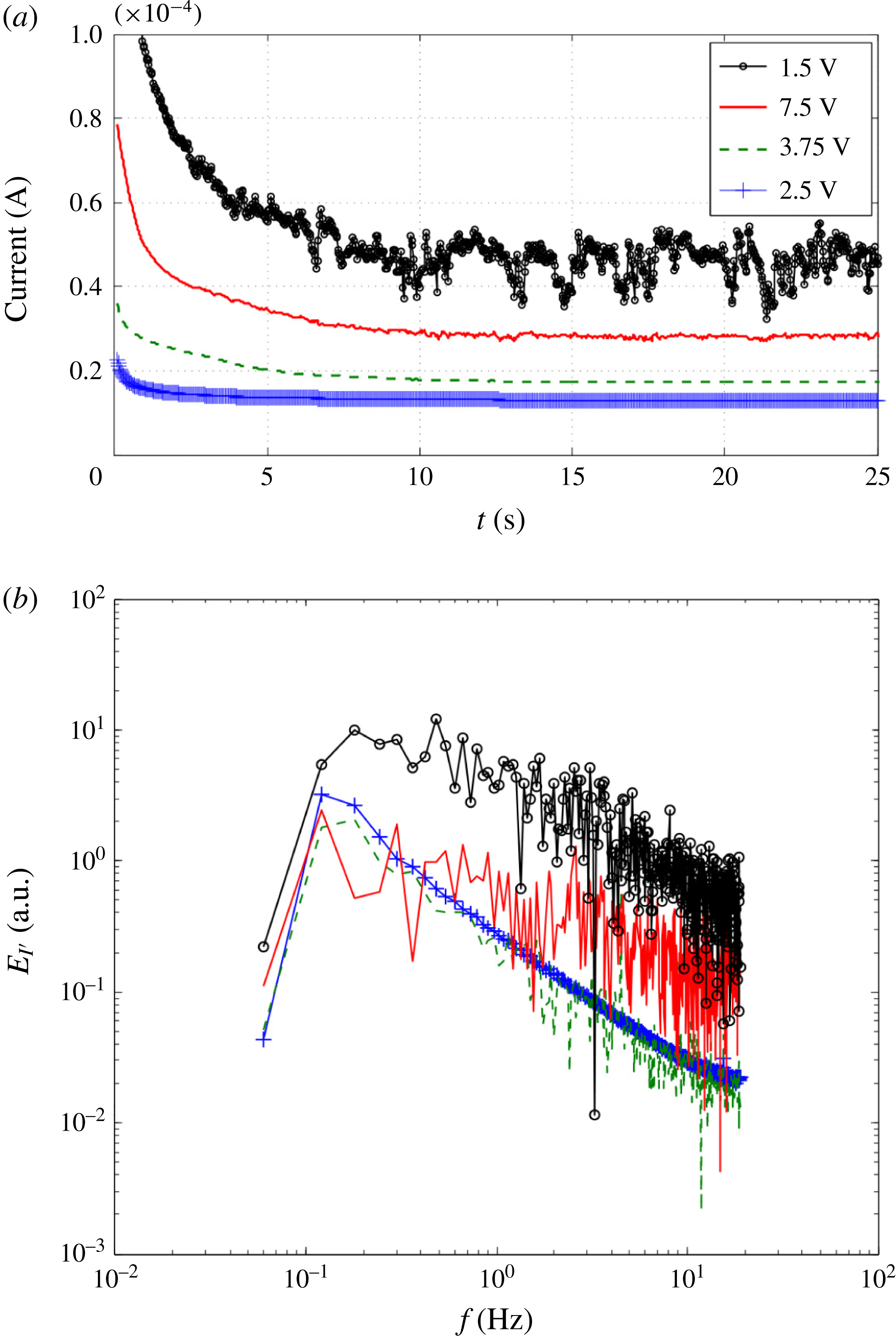
(a) The current–time responses. The currents were recorded for 25 s in 26.5 ms increments. (b) The power spectra of current noise at 2.5–15 V and
 $5~\unicode[STIX]{x03BC}\text{L}~\text{min}^{-1}$
(the fluorescent images are available in figure 4
a). Each case indicates linear ICP (2.5 V), EC in the diffusion layer (3.75 V), stable EC (7.5 V) and chaotic EC (15 V).

4.4 Noise reduction in chaotic EC: vortex sweeping
We discover the mechanism of noise reduction in chaotic EC by analysing the power spectra of the current noise (figures 8 and 9). Similarly to the power spectrum of the fluorescent intensity, the current–time responses were measured and normalized by the mean values after saturation (
 ${>}10$
s, figure 8
a). The noise spectra also represent the four ICP regimes (figure 8
b). The linear ICP has a smooth current–time response and a background noise spectrum without EC vortices (2.5 V). At 3.75 V, a slight disturbance is observed in the current–time curve, and the spectrum represents this as disturbances in a high-frequency range (
 $f>1$
Hz). The shape of the spectrum is not changed here. As stable and chaotic ECs change the shape of the boundary layer (7.5–15 V), current fluctuations are manifested and the noise levels of the spectra also increase.
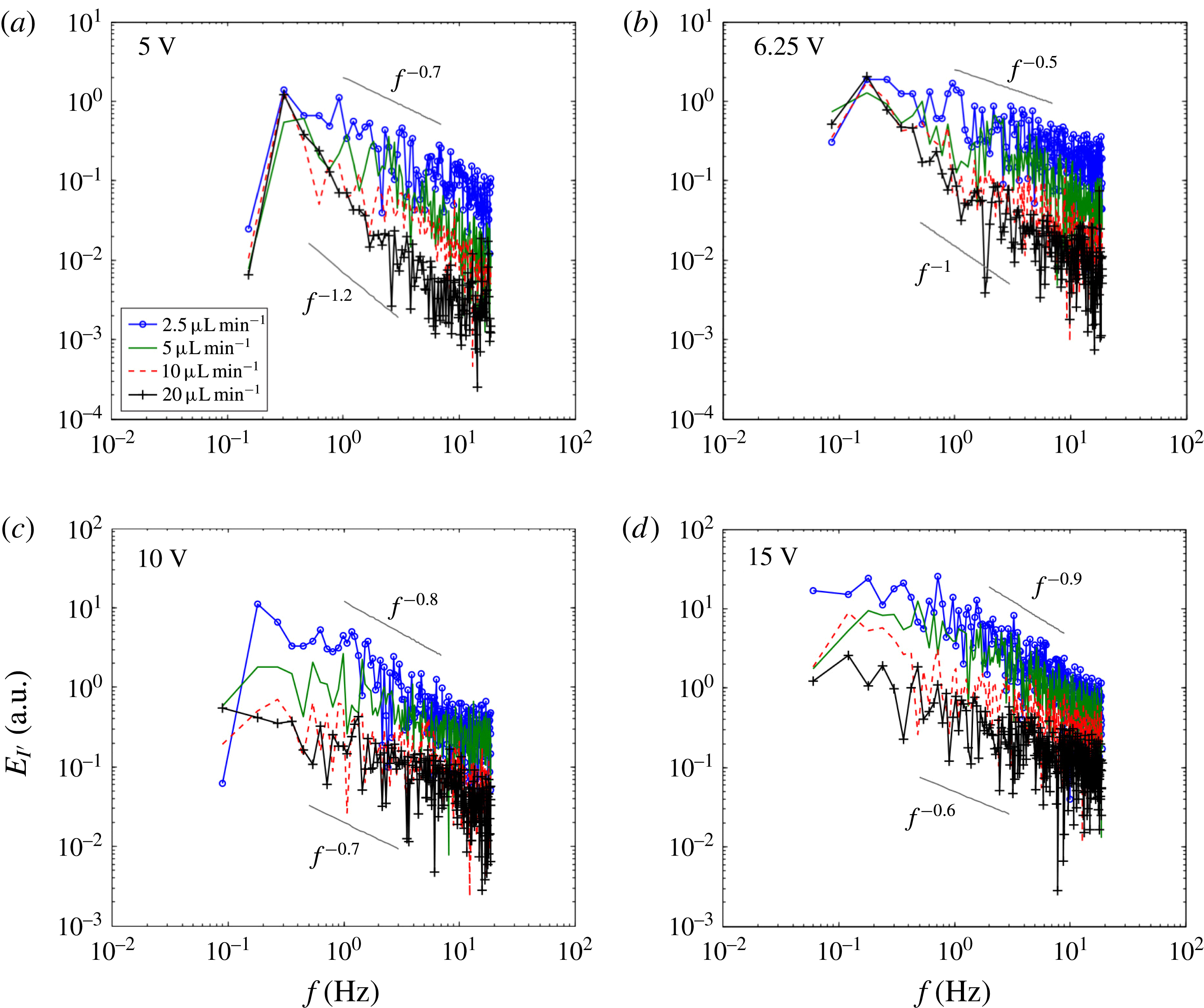
More importantly, this noise spectrum allows us to identify the two effects of pressure-driven flow on EC: shear sheltering (shear-related) and vortex sweeping (shear-independent) (figure 9). As addressed in Terry (Reference Terry2000b
), shear sheltering occurs when the flow-shear rate exceeds a vortex rotation period (i.e. eddy lifetime or turnover time); the flow shear stretches and breaks up vortices. At 5–6.25 V and 2.5–
 $20~\unicode[STIX]{x03BC}\text{L}~\text{min}^{-1}$
, stable EC changes its vortex size without altering to chaotic EC (figure 9
a,b). In this case, the noise spectra only shift in the high-frequency regime (
 $f>$
1 Hz), where frequencies higher than those of stable EC exist (figure 4
c). At a higher flow rate and/or a lower voltage, the size of the stable EC decreases, and the high-frequency noise is reduced. However, the spectra are tied up in the low-frequency regime (
 $f<1$
Hz). This is because a larger size of perturbations could not occur over the thickness of the flow-shear-induced transport barrier. As a result, we can observe slope changes of the spectrum: the slope is almost doubled from 20 to 2.5
 $\unicode[STIX]{x03BC}\text{L}~\text{min}^{-1}$
at fixed voltages (5 and 6.25 V, figure 9
a,b). In contrast, vortex sweeping indicates that the fast mean flow literally sweeps vortices (Shats et al.
Reference Shats, Xia, Punzmann and Falkovich2007). In other words, shear sheltering decorrelates vortices, whereas vortex sweeping reduces the degree of vortical fluid motion by pushing the vortices in the flow-wise direction quickly. The degree of sweeping is then fair to all sizes of eddies at a given flow velocity. Accordingly, the noise spectrum shifts globally without slope changes (10–15 V, figure 9
c,d). Shats et al. (Reference Shats, Xia, Punzmann and Falkovich2007) also observed that the vortex sweeping induced the overall spectrum shift of the turbulent kinetic energy in electromagnetic flows.
It is noteworthy that shear sheltering and vortex sweeping are not in coexistence in this system. The vortex sweeping effect is negligible for the stable EC cases where the vortices are sheltered by the flow shear (5–6.25 V, figure 9
a,b). On the other hand, this sweeping effect dominates for the chaotic EC cases, when the vortices overcome the shear suppression and expand over
 $d_{EC}/w>0.618$
(10–15 V, figure 9
c,d). This is due to the fact that the vortex sweeping dominates in the middle of the channel (with a high flow velocity) and becomes weaker near the wall (with a low flow velocity, figure 3). Stable EC (and the transport barrier) always occurs in a high-shear region near the wall, so it is free from the sweeping effect. When EC vortices come out of this high-shear region (i.e. chaotic EC), the fast mean flow starts to sweep the vortices near the middle of the channel.
The power spectra of current noise at 5–15 V and 2.5–
 $20~\unicode[STIX]{x03BC}\text{L}~\text{min}^{-1}$
. (a–b) At 5–6.25 V, stable EC occurs for all flow rates, except for the
 $20~\unicode[STIX]{x03BC}\text{L}~\text{min}^{-1}$
cases (EC in the diffusion layer). (c–d) At 10–15 V, chaotic EC occurs for all flow rates, except at 10 V and
 $20~\unicode[STIX]{x03BC}\text{L}~\text{min}^{-1}$
(stable EC).

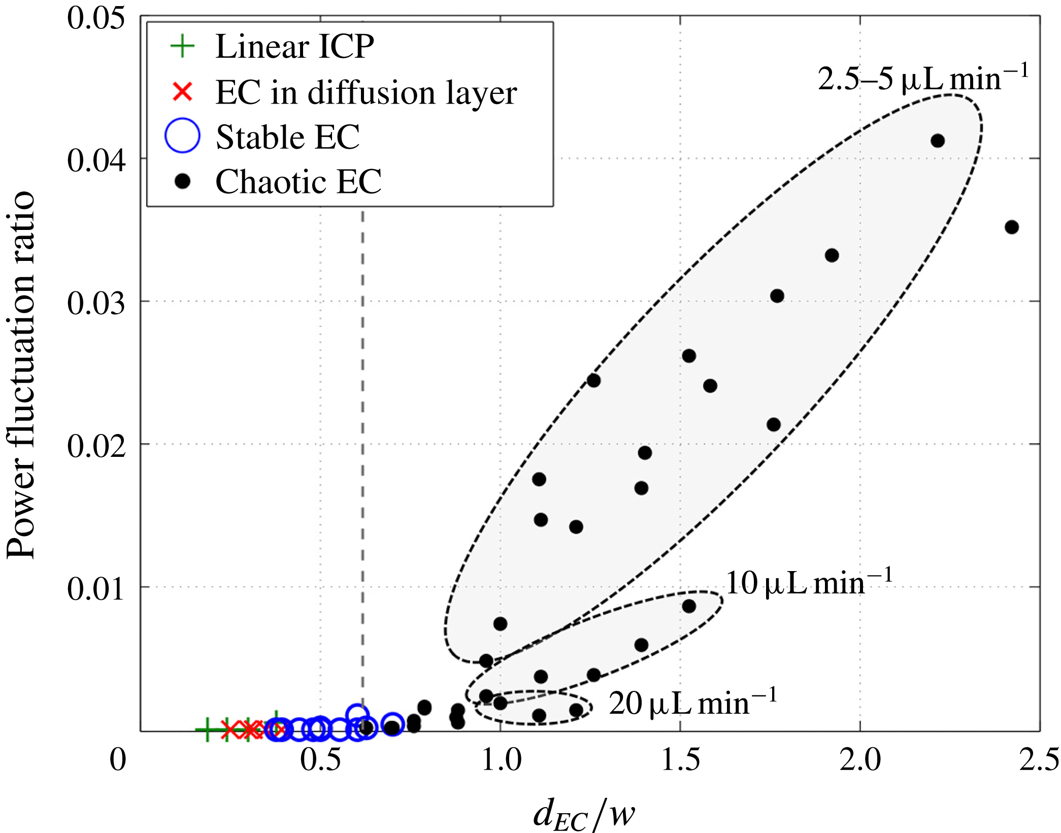
In the integrated view, the trend of electrical power fluctuation shows the bifurcation of stable/chaotic EC (by shear sheltering) and the noise reduction of chaotic EC (by vortex sweeping) (figure 10). The ratio of the electric power fluctuation
 $P^{\prime }$
to the averaged power
 $\bar{P}$
is calculated as
 $I^{\prime 2}/\bar{I}^{2}$
, where
 $I^{\prime }$
is the current fluctuation (
 $=$
the standard deviation of the current in figure 4
b) and
 $\bar{I}$
is the averaged current. Arranged in
 $d_{EC}/w$
, the power fluctuation ratio
 $P^{\prime }/\bar{P}$
emerges as chaotic EC is initiated. The ratio under the threshold (
 $d_{EC}/w<0.618$
) is not over 0.1 % even with stable EC. With chaotic EC, however, the power fluctuation ratio increases rapidly to 4 %. Interestingly, we identify three distinct groups in the chaotic EC regime according to the flow velocity. Even with a similar height of the EC vortex, a high flow velocity can sweep the vortices and reduce the power fluctuation. The fluctuation ratio is capped after
 $d_{EC}/w=2$
, because the EC height
 $d_{EC}$
is physically limited by the finite channel width
 $2w$
. In addition, with the decomposed quantities (measured current
 $\tilde{I} =\bar{I}+I^{\prime }$
), we can consider that
 $P^{\prime }$
and
 $\bar{P}$
correspond to the electric power consumption and the viscous dissipation of the power respectively. The power fluctuation ratio in this experiment (stable
 $\text{EC}<0.1\,\%$
, chaotic
 $\text{EC}<4\,\%$
) is well matched with the previous numerical result for non-sheared stable/chaotic EC in a stationary reservoir; the power losses by the viscous dissipation of the stable/chaotic ECs are 0.1 % and 4 % respectively (Druzgalski et al.
Reference Druzgalski, Andersen and Mani2013).
The power fluctuation ratio. The ratio of the electric power fluctuation
 $P^{\prime }$
to the averaged power
 $\bar{P}$
is enumerated with the height of the EC vortex
 $d_{EC}/w$
. Without chaotic EC, there is no deviation as the flow rate changes. The dotted line indicates
 $d_{EC}/w=0.618$
.

4.5 Scaling in ion convection by sheared EC
For practical applications, it is important to identify how much the ion flux is enhanced by EC vortices, especially under shear flow. To this end, we define the electric Nusselt number
 $Nu_{E}$
as the ratio of the overall (
 $\text{convection}+\text{conduction}$
) and conductive ion fluxes. Stable/chaotic EC drives the ion flux convectively, and electromigration under the electric field drives the ion flux conductively. The ion exchange membrane is hydrodynamically non-permeable. The convection term is therefore converted to the conduction term at the membrane. The convection by EC increases the ion concentration gradient and the local electric field, and enhances the conductive ion fluxes on the membranes (Kwak et al.
Reference Kwak, Pham, Lim and Han2013b
). From the Nernst–Plank equations (3.2), if the diffusion term is negligible, the theoretical
 $Nu_{E}$
can be presented as
 $$\begin{eqnarray}Nu_{E-1}=\frac{FzC\boldsymbol{u}}{\displaystyle \frac{F^{2}}{RT}z^{2}CD_{eff}\unicode[STIX]{x1D735}\unicode[STIX]{x1D719}}=\frac{RT}{Fz}\boldsymbol{\cdot }\frac{\boldsymbol{u}}{D_{eff}\unicode[STIX]{x1D735}\unicode[STIX]{x1D719}}.\end{eqnarray}$$
Substituting
 $\boldsymbol{u}=u_{EC}\sim (\unicode[STIX]{x1D716}/\unicode[STIX]{x1D707})(V^{2}/d_{EC})$
and
 $\unicode[STIX]{x1D735}\unicode[STIX]{x1D719}=E\sim V/d_{EC}$
into (4.7), we obtain
 $$\begin{eqnarray}Nu_{E}-1=\frac{RT}{Fz}\cdot \frac{\unicode[STIX]{x1D716}V}{\unicode[STIX]{x1D707}D_{eff}}.\end{eqnarray}$$
Recalling the scaling law for Rayleigh–Benard convection (Grossmann & Lohse Reference Grossmann and Lohse2000; Stevens et al.
Reference Stevens, van der Poel, Grossmann and Lohse2013), we can represent
 $Nu_{E}$
with the electric Rayleigh number
 $Ra_{E}$
and the Reynolds number
 $Re$
. In accordance with the definitions in the previous sections,
 $$\begin{eqnarray}\displaystyle & \displaystyle Ra_{E}=\frac{\unicode[STIX]{x1D716}E^{2}(2w)^{2}}{\unicode[STIX]{x1D707}D_{eff}}=\frac{4\unicode[STIX]{x1D716}V^{2}}{\unicode[STIX]{x1D707}D_{eff}}\left(\frac{d_{EC}}{w}\right)^{-2}, & \displaystyle\end{eqnarray}$$
 $$\begin{eqnarray}\displaystyle & \displaystyle Re_{DH}=\frac{\unicode[STIX]{x1D70C}U_{HP}D_{H}}{\unicode[STIX]{x1D707}}. & \displaystyle\end{eqnarray}$$
Substituting
 $Ra_{E}$
and
 $Re_{DH}$
with the scaling law for the vortex height
 $d_{EC}/w=[(\unicode[STIX]{x1D716}D_{H}^{2}/64\unicode[STIX]{x1D707}w^{3})(V^{2}/U_{HP})]^{1/3}$
, the relationship between
 $Nu_{E},Ra_{E}$
and
 $Re_{DH}$
is obtained:
 $$\begin{eqnarray}Nu_{E}-1=\left(\frac{RT}{Fz}\cdot \frac{\unicode[STIX]{x1D70C}\unicode[STIX]{x1D716}^{1/2}D_{eff}^{1/2}D_{H}^{3}}{16\unicode[STIX]{x1D707}^{3/2}w^{3}}\right)\frac{Ra_{E}^{3/2}}{Re_{DH}}.\end{eqnarray}$$
If we consider the critical
 $Ra_{E}$
for initiating EC vortices,
 $$\begin{eqnarray}Nu_{E}-1\sim \frac{(Ra_{E}-Ra_{E_{crit}})^{3/2}}{Re_{DH}}.\end{eqnarray}$$
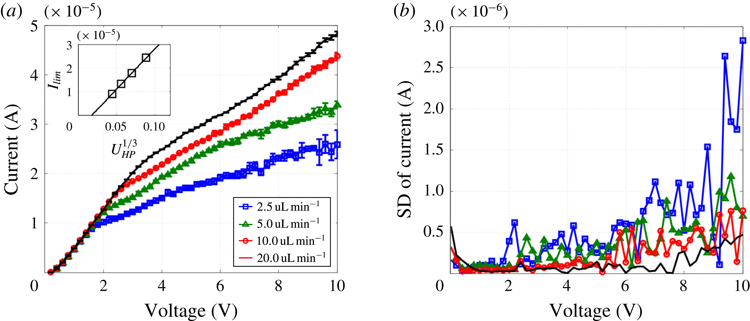
To confirm this scaling analysis, the limiting current
 $I_{lim}$
was measured from the current–voltage curves (figure 11). In the Ohmic regime (
 ${<}2$
V), the slope of the curves is the electric conductance
 $G$
, which is the same for all flow rates (
 $G=5.97~\unicode[STIX]{x03BC}\text{S}$
). However, the limiting current
 $I_{lim}$
depends on the flow velocity
 $U_{HP}$
; according to the conventional convective-diffusion model (Probstein Reference Probstein2003), the limiting current is proportional as
 $I_{lim}\sim U_{HP}^{1/3}$
. This tendency is also presented in this experiment (figure 11
a). Similarly to the current–time responses (figure 8
a), there is no visible current deviation, with no or negligible EC in the Ohmic-limiting regimes (
 ${<}2$
–3 V, figure 11
a,b). However, current deviations appear with stable/chaotic EC in the overlimiting regime (
 ${>}3$
V). This current deviation also becomes stronger at lower flow rates and/or higher voltages; that is, chaotic EC shows a stronger current fluctuation than stable EC, and this fluctuation becomes more intense as chaotic EC becomes more chaotic.
Current–voltage responses. (a) Current–voltage (
 $I{-}V$
) curves and (b) the standard deviations (SDs) of the currents under various flow rates (2.5–20
 $\unicode[STIX]{x03BC}\text{L}~\text{min}^{-1}$
). The current responses were measured four times by ramping the voltage up with 0.2 V steps from 0 to 10 V with 30 s delay. We then averaged the current values and calculated the SDs of the current. The inset graph in (a) indicates the relationship between the limiting current
 $I_{lim}$
and the flow velocity
 $U_{HP}$
. The limiting currents were selected at the knee points of the curves (8.86, 13.15, 17.77 and 2.42
 $\unicode[STIX]{x03BC}\text{A}$
).

The
 $Nu_{E}$
–
 $Ra_{E}$
curves for various flow rates (2.5–20
 $\unicode[STIX]{x03BC}\text{L}~\text{min}^{-1}$
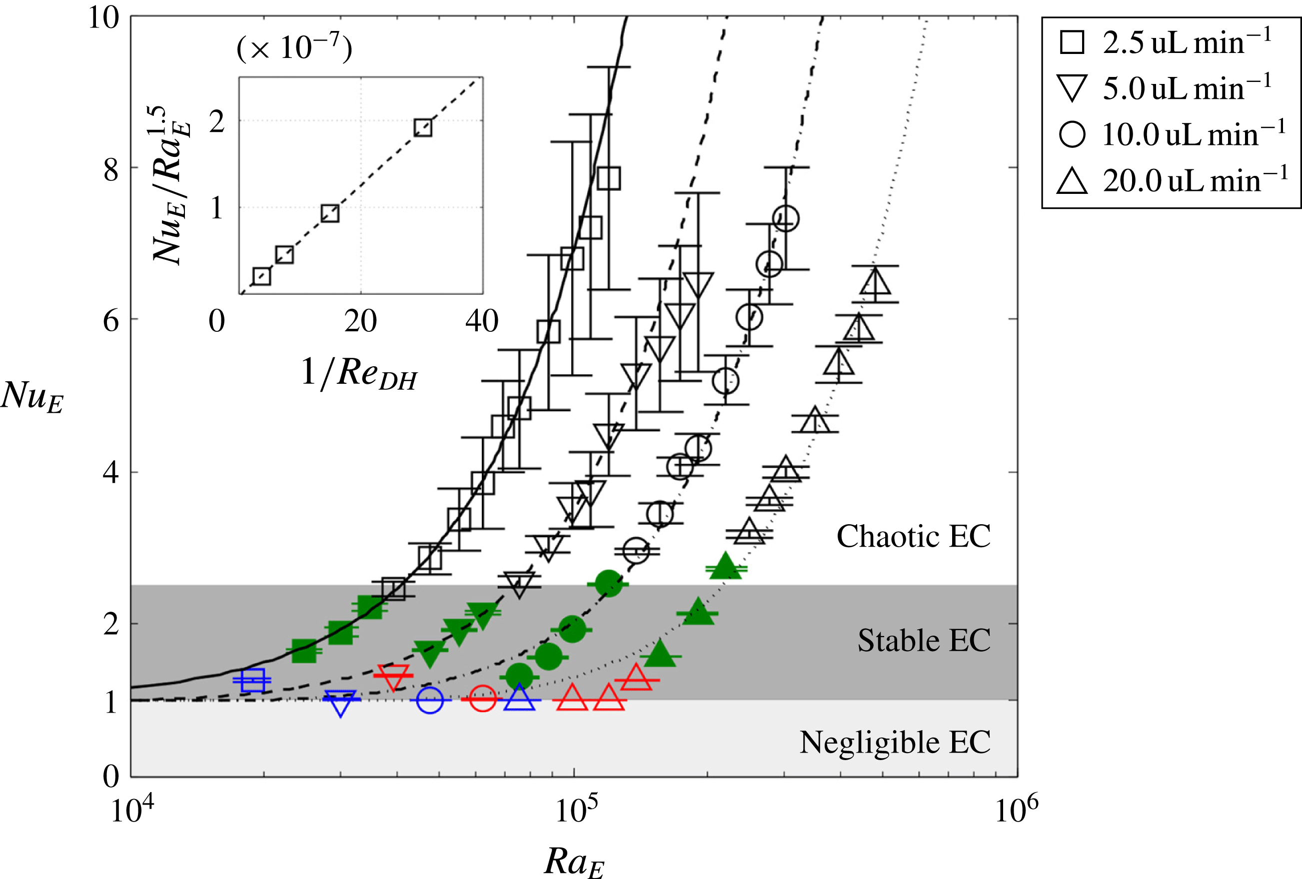
) and applied voltages (2.5–40 V). The blue, red, green and black points indicate the four ICP regimes (linear ICP, EC in diffusive layer, stable EC and chaotic EC) respectively. The equations of the fitting curves are
 $y=1.91\times 10^{-7}(x-1225)^{1.5}+1,y=9.18\times 10^{-8}(x-9242)^{1.5}+1,y=4.43\times 10^{-8}(x-18\,898)^{1.5}+1$
and
 $y=1.98\times 10^{-8}(x-38\,537)^{1.5}+1$
for 2.5–
 $20~\unicode[STIX]{x03BC}\text{L}~\text{min}^{-1}$
respectively;
 $R^{2}=0.99$
for all curves. The inset graph shows the linearity between the slope of the fitting curves and
 $1/Re_{DH}$
.

Now, we can calculate the electric Nusselt number in experiments as
 $Nu_{E}=I/I_{lim}$
in the overlimiting regime. The electric Nusselt number
 $Nu_{E}$
(
 $=I/GV$
) is always 1 in the Ohmic-limiting regimes, because the overall ion flux is induced only by electromigration (figure 12). We plot the experimental results in the
 $Nu_{E}$
–
 $Ra_{E}$
plane, and the scaling law (
 $y=A(x-B)^{1.5}+1$
, equation (4.12)) exactly follows the data points. The slope of the fitting curve (
 $A$
) is proportional to
 $Re_{DH}^{-1}$
(inset image in figure 12). As we have already confirmed, a higher
 $Ra_{E}$
(
 $B$
) is required to initiate stable EC and also to initiate chaotic EC (to overcome the flow shear) under a higher flow velocity. The stable and chaotic EC cases are smoothly connected at a given flow rate. This indicates that the global trends are maintained in both states with the same scaling laws for the vortex height (Kwak et al.
Reference Kwak, Pham, Lim and Han2013b
) and the convective ion flux (4.12). It is also noted that the
 $Nu_{E}$
of stable EC is limited to
 ${\sim}2.5$
. This is presumably because the limited size of vortices (
 $d_{EC}/w<0.618$
) can convect a limited amount of ions.
4.6 Stable and chaotic EC in numerical simulation
Lastly, we reproduce the shear sheltering of EC in the two-dimensional simulation model (figure 13). The average velocity of the HP flow is
 $U_{HP}=800U_{0}-1600U_{0}$
(
 $U_{0}=9.887~\unicode[STIX]{x03BC}\text{m}~\text{s}^{-1}$
) and the applied voltage between the two CEMs is
 $V=26{-}45\unicode[STIX]{x1D719}_{0}$
(
 $\unicode[STIX]{x1D719}_{0}=25.85$
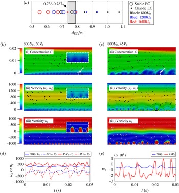
mV). Figure 13(a) shows the phase diagram of stable/chaotic EC enumerated by
 $d_{EC}/w$
. At
 $d_{EC}/w=0.736{-}0.787$
, the numerical calculation also accurately captures the bifurcation of stable and chaotic EC. The relatively large threshold offset (from 0.618) is due to the small geometry with a thicker portion of the electric double layer, which induces an offset between the actual and calculated EC heights (supporting information figure 2b).
In figure 13(b–c), we observe the characteristics of the EC vortices minutely by mapping concentration profiles (i), velocity fields (ii) and vorticity (iii) with flow streamlines (black or white solid lines). The high coherence of stable EC is represented with uniform circular depletion zones, high-velocity zones and positive-vorticity zones on the lower CEM (figure 13
b). At the valley of the vortices, the inflow towards the CEM suppresses the depletion zone; then, the flow turns in a counter-clockwise direction, inducing a fast velocity and a positive vorticity (white dotted boxes in figure 13(b)). In contrast, chaotic EC shows rambling patterns along the membrane (figure 13
c). Consequently, as we hypothesized and visualized experimentally, the advection of stable (chaotic) EC generates weak periodic (strong chaotic) velocity/vorticity fluctuations at the fixed location on the EC boundary (white dotted arrow in figure 13(b,c)) (figure 13
d,e). Here, we also can check the degree of vortex sweeping. The magnitude of the velocity fluctuation is approximately
 $320U_{0}$
by stable EC and
 $465U_{0}$
by chaotic EC. At the stable EC boundary (
 $y\sim 0.06l_{0}$
), the velocity by the HP flow is
 ${\sim}270U_{0}$
, which is smaller than that of stable EC. In contrast, chaotic EC expands to
 $y\sim 0.18l_{0}$
, where the velocity by the HP flow is far over the chaotic EC speed (
 ${\sim}812U_{0}$
). If we define the sweeping rate as the ratio of the EC speed and the HP velocity at the EC boundary, the sweeping rate of chaotic EC (
 $=1.75$
) is two times larger than that of stable EC (
 $=0.84$
). This tendency is well matched with the experimental observation in the current noise spectra.
Two-dimensional numerical simulation of stable and chaotic EC. (a) Phase diagram for 15 simulation tests. Here,
 $d_{EC}/w$
is calculated using
 $d_{EC}/w=0.1807(V^{2}/U_{HP})^{1/3}$
, where
 $D_{H}=4w=120~\unicode[STIX]{x03BC}\text{m}$
(channel height
 $h\sim \infty$
). The bifurcation of stable and chaotic EC occurs at
 $d_{EC}/w=0.736{-}0.787$
(grey box). Local dimensionless properties with (b) stable and (c) chaotic EC: (i) ion concentration (
 $C$
), (ii) velocity field (
 $u_{x}$
in the
 $x$
-direction,
 $u_{y}$
in the
 $y$
-direction) and (iii) vorticity (
 $w_{z}$
in the
 $z$
-direction). The colour bars indicate the range of ion concentration (
 $0{-}0.02C_{0},C_{0}=10~\text{mM}$
), velocity (
 $0{-}1600U_{0},U_{0}=9.887~\unicode[STIX]{x03BC}\text{m}~\text{s}^{-1}$
), and vorticity (
 $-1000f_{0}$
–
 $1000f_{0}$
,
 $f_{0}=l_{0}/U_{0}=60~\unicode[STIX]{x03BC}\text{m}/9.887~\unicode[STIX]{x03BC}\text{m}~\text{s}^{-1}$
). Enlarged images are shown in the white dotted boxes. (d–e) At the specific point
 $x=2l_{0},y=0.06l_{0}$
(white dotted arrow in (b–c), where the origin is at the left bottom corner), the spatial perturbations by the EC vortices can translate to the temporal perturbations as the vortices advect in the flow-wise direction.

5 Conclusion
In this paper, we combined three independent approaches (experiment, numerical simulation and scaling analysis) to verify the existence of shear sheltering observed in many electrochemical devices, i.e. EC under shear flow on ion exchange membranes. We found that stable EC with coherent unidirectional vortices is completely transformed to chaotic EC with spatiotemporal chaotic eddies, and recognized that this transition is delayed under high flow shear. Beyond this phenomenological representation of shear sheltering, we discovered the threshold for stable and chaotic EC by scaling analysis. Applying the classic shear sheltering model, it was found that the magnitude of the velocity perturbation by stable EC is balanced by the flow shear when the EC height is
 $d_{EC}/w=0.618$
. This result suggests that a strong pressure-driven flow can confine the velocity/vorticity fluctuations of EC in the high-shear region (
 $d_{EC}/w<0.618$
), realizing stable unidirectional vortices. On the other hand, if the EC vortices are strongly developed with their height over the threshold (
 $d_{EC}/w>0.618$
), the vortices become chaotic by overwhelming the flow shear. The scaling law to determine the transition threshold was validated by both experiments and numerical simulation, and can be utilized as a design guide to prevent chaotic flows and corresponding power dissipation in electrochemical applications.
In addition, we quantified the periodicity and chaoticity of the sheared EC by visualizing attractors in a time-delay phase space. Four different ICP regimes including stable and chaotic EC were observed with steady, periodic and chaotic attractors respectively. The illustration of attractors near the threshold (
 $d_{EC}/w=0.703$
) also presented the subharmonic and weak chaotic states between the periodic and fully chaotic states. Here, we discovered that vortex sweeping also existed, and this shear-independent effect can reduce the chaotic level of chaotic EC. The two effects of the pressure-driven flow (shear sheltering and vortex sweeping) were clearly decoupled in the power spectra of current noise and the electric power fluctuation. The shear sheltering determines the slope of the current noise spectra and the onset of the electric power fluctuation. While the EC vortices are in the flow-shear-induced transport barrier, the vortex sweeping is negligible with a low flow velocity. On the other hand, this sweeping effect becomes dominant when the vortices come out of the barrier and are exposed to a high flow velocity. Consequently, the noise spectra shift without slope change, and the electric power fluctuation bifurcates according to the flow velocity. These two effects also successfully explain the ion convection by the sheared EC with the new power law for the electric Nusselt number. Based on this detailed study, one can understand the interaction between the shear flow and the EC vortices, which can be utilized as a design guide to prevent chaotic flows and corresponding power dissipation in electrochemical applications.
Acknowledgements
This work was supported by ARPA-E Award DE-AR0000294. It was also supported by the Signature Project on Brine Management, which was funded by Kuwait Foundation for the Advancement of Sciences (KFAS). R.K. was supported by the institutional program in the Korea Institute of Science and Technology (2E26633). V.S.P. was partially supported by SMART Centre, Singapore (BioSyM IRG).
Supplementary data and movies
Supplementary data and movies are available at https://doi.org/10.1017/jfm.2016.870.