2.1 Jet parameters

Four large-eddy simulations of a jet impinging on a flat plate normally are performed. The jet originates from a planar straight nozzle of height $h$ and width $l=3.25h$ in the spanwise direction. The lip thickness is $e=0.5h$ and periodic conditions are imposed in the spanwise direction. Nozzle-to-plate distances $L$ equal to $3.94h$ , $5.5h$ , $8.27h$ and $9.1h$ are considered. The four cases are consequently referred to as JetL3.9, JetL5.5, JetL8.3 and JetL9.1. The ejection conditions of the jet and the nozzle-to-plate distances are similar to those in the experimental study of Thurow et al. (Reference Thurow, Samimy and Lempert2002). Thus, the jet is ideally expanded, and has a Mach number of ${\mathcal{M}}_{j}=u_{j}/a_{j}=1.28$ , where $u_{j}$ is the jet exit velocity and $a_{j}$ is the speed of sound at the nozzle exit. The jet Reynolds number is $Re_{h}=u_{j}h/\unicode[STIX]{x1D708}=5\times 10^{4}$ , where $\unicode[STIX]{x1D708}$ is the kinematic molecular viscosity. At the nozzle exit, a Blasius boundary-layer mean velocity profile of $0.075h$ wide is imposed. Finally, low-amplitude random vortical disturbances not correlated in the spanwise direction are added in the boundary layer in the nozzle $0.25h$ upstream from the exit in order to generate velocity fluctuations at the nozzle exit. The strength $\unicode[STIX]{x1D6FC}$ of the forcing is similar to those used in Bogey, Marsden & Bailly (Reference Bogey, Marsden and Bailly2011). It is set to 0.02, allowing us to reach peak turbulent intensities between 5 % and 10 % at the nozzle exit, as it will be reported in the next section.

2.2 Numerical parameters

The unsteady compressible Navier–Stokes equations are solved on a Cartesian mesh for which $x$ , $y$ and $z$ denote the longitudinal, lateral and spanwise directions, respectively. An explicit six-stage Runge–Kutta algorithm is used for time integration, and low-dispersion eleven-point explicit centred finite differences are employed for spatial derivation (Bogey & Bailly Reference Bogey and Bailly2004; Berland et al. Reference Berland, Bogey, Marsden and Bailly2007b ). At the end of each time step, a sixth-order eleven-point filtering (Bogey, de Cacqueray & Bailly Reference Bogey, de Cacqueray and Bailly2009) is applied to the flow variables in order to remove grid-to-grid oscillations and to relax turbulent energy from scales at wavenumbers close to the grid cutoff wavenumber. Thus, the filtering acts as a subgrid-scale model in the LES (Bogey & Bailly Reference Bogey and Bailly2006, Reference Bogey and Bailly2009; Fauconnier, Bogey & Dick Reference Fauconnier, Bogey and Dick2013; Kremer & Bogey Reference Kremer and Bogey2015). The radiation conditions of Tam & Dong (Reference Tam and Dong1994) are implemented at the upstream and lateral boundaries of the computational domain. A sponge zone combining grid stretching and Laplacian filtering is also used to damp the turbulent fluctuations before they reach the lateral boundaries. This numerical set up has been used in past studies to simulate round subsonic jets at ${\mathcal{M}}_{j}=0.9$ (Bogey et al. Reference Bogey, Marsden and Bailly2011; Bogey, Marsden & Bailly Reference Bogey, Marsden and Bailly2012; Bogey & Marsden Reference Bogey and Marsden2016) and an underexpanded planar jet at a fully expanded Mach number of ${\mathcal{M}}_{j}=1.55$ (Berland, Bogey & Bailly Reference Berland, Bogey and Bailly2007a ) for instance. In the present LES, adiabatic conditions are imposed at the nozzle walls and the flat plate. A shock-capturing filtering is applied in order to avoid Gibbs oscillations near shocks. It consists of applying a conservative second-order filter at a magnitude determined each time step using a shock sensor (Bogey et al. Reference Bogey, de Cacqueray and Bailly2009). This method was successfully used by de Cacqueray, Bogey & Bailly (Reference de Cacqueray, Bogey and Bailly2011) for the LES of an overexpanded jet at ${\mathcal{M}}_{j}=3.3$ .

Figure 1.

Representation of (a) the lateral mesh spacings and (b) the axial mesh spacings: —— JetL3.9, — ⋅ — JetL5.5, – – – JetL8.3 and 

 JetL9.1.

Table 1.

Parameters of the grids.

The simulations are carried out using an OpenMP-based in-house solver, and a total of 200 000 iterations are computed in each case after the transient period. The temporal discretization is equal to $\unicode[STIX]{x0394}t=0.0025h/u_{j}$ , yielding a simulation time of $500h/u_{j}$ . The parameters of the Cartesian grids used in the four LES are reported in table 1. The grids contain between 184 and 263 million points. The variations of the axial and lateral mesh spacings are represented in figure 1. The minimal axial mesh spacing, near the nozzle lip and the flat plate, is set to $\unicode[STIX]{x0394}x=0.00375h$ , and the maximal axial mesh spacing is $\unicode[STIX]{x0394}x=0.015h$ . The lateral mesh spacings are equal to $\unicode[STIX]{x0394}y=0.00375h$ at $y=\pm h/2$ and to $\unicode[STIX]{x0394}y=0.03h$ for $2.5h\leqslant y\leqslant 8h$ . Finally, a number of 219 points are used in the spanwise direction, giving a mesh spacing $\unicode[STIX]{x0394}z=0.015h$ . The maximum mesh spacing of $0.03h$ allows acoustic waves to be well calculated up to the Strouhal number $St=fh/u_{j}=5.6$ , where $f$ is the frequency. Note, moreover, that in the physical domain the grids are stretched at rates lower than 1 % in order to preserve numerical accuracy.

3.1 Flow snapshots

Three-dimensional isosurfaces of density are represented in figure 2 for JetL3.9 and JetL9.1 in order to visualize the shear layers of the jets. Both small- and very large-scale structures are visible. The near acoustic fields obtained in the plane $(x,y)$ are also shown. For the two jets, acoustic waves appear clearly to come from the region of jet impact.

Figure 2.

Representation for (a) JetL3.9 and (b) JetL9.1 of the isosurfaces of density associated with $1.25~\text{kg}~\text{m}^{-3}$ , coloured by the local Mach number, and of the pressure fluctuations in the plane $(x,y)$ using a colour scale ranging from $-7500$ to 7500 Pa, from white to red. The nozzle and the flat plate are in grey.

Snapshots of the vorticity norm obtained in the plane $(x,y)$ and in the plane $(x,z)$ at $y=-h/2$ , are represented in figure 3. For JetL3.9, the two shear layers exhibit in the $(x,y)$ plane large-scale structures, of typical size $0.5h$ , which do not seem to be organized symmetrically with respect to the jet axis. In the spanwise direction, large- and small-scale structures, namely vorticity tubes along the entire spanwise extent and structures of typical size $0.05h$ , can both be seen. Besides, the spanwise correlation of the flow structures appears significant near the nozzle but also near the flat plate. For JetL5.5, JetL8.3 and JetL9.1, large-scale structures are still visible in the shear layers, but their spanwise correlations is relatively weak far from the nozzle. Overall, however, a nearly two-dimensional organization of the vortical structures is visible in the shear layers, as observed experimentally for supersonic rectangular impinging jets by Krothapalli (Reference Krothapalli1985) and Norum (Reference Norum1991) and by Thurow et al. (Reference Thurow, Samimy and Lempert2002) using real-time flow visualization techniques.

Figure 3.

Snapshots in the plane $(x,y)$ and in the plane $(x,z)$ at $y=-h/2$ of the vorticity norm $|\unicode[STIX]{x1D714}|$ for (a) JetL3.9, (b) JetL5.5, (c) JetL8.3 and (d) JetL9.1. The colour scale ranges up to the level of $10u_{j}/h$ , from white to red. The nozzle is in black.

Density and fluctuating pressure fields obtained in the $(x,y)$ plane for the four jets are provided in figure 4 and movie 1 available at https://doi.org/10.1017/jfm.2016.628. In all cases, large-scale structures and sound waves are observed in the shear layers and outside the jet, respectively. For JetL3.9 and JetL5.5, the pressure waves come from the region of jet impact, and are organized antisymmetrically with respect to the jet axis. For JetL8.3 and JetL9.1, two acoustic components appear in the pressure fields. The first components consist of circular waves centred around $x\simeq 2h$ in the jet shear layers. The second components propagate from the region of jet impact, mostly in the upstream direction. They are similar but weaker than those observed for JetL3.9 and JetL5.5.

Figure 4.

Snapshots in the $(x,y)$ plane of the density in the jet and close to the flat plate and of the pressure fluctuations for (a) JetL3.9, (b) JetL5.5, (c) JetL8.3 and (d) JetL9.1. The colour scale ranges from 1 to $2~\text{kg}~\text{m}^{-3}$ for density, from blue to red and from $-7500$ to 7500 Pa for pressure, from black to white. The nozzle is in black.

3.2 Mean flow fields

Mean velocity fields obtained in the $(x,y)$ plane are shown in figure 5. As expected, very small variations, of only approximately 4 % of the jet exit velocity, are noted near the axis, indicating that the jets are almost ideally expanded. In all cases, a stagnation point is visible on the flat plate at $y=0$ , and two plane wall jets are created after the jet impact. Important parameters of wall jets include the maximum velocity $u_{max}$ , the distance $x_{max}$ from the wall at which the velocity reaches $u_{max}$ and the distance $x_{1/2}$ at which the velocity has dropped to $u_{max}/2$ , refer to Irwin (Reference Irwin1973) and George et al. (Reference George, Abrahamsson, Eriksson, Karlsson, Löfdahl and Wosnik2000) for instance. The values calculated at $y=2h$ for the present wall jets are given in table 2. For a greater nozzle-to-plate distance, the wall jet maximum velocity is found to be lower, as expected. In parallel, the wall jet thickness $x_{max}$ is smaller, whereas the wall jet thickness $x_{1/2}$ is larger.

Figure 5.

Mean velocity field obtained in the $(x,y)$ plane for (a) JetL3.9, (b) JetL5.5, (c) JetL8.3 and (d) JetL9.1. The colour scale ranges from 0 to $400~\text{m}~\text{s}^{-1}$ , from blue to red. The nozzle is in black.

Figure 6.

Axial variations of the peak root-mean-square values of velocity fluctuations (a)  $u^{\prime }$ and (b)  $v^{\prime }$ for —— JetL3.9, — ⋅ — JetL5.5, – – – JetL8.3 and 

 JetL9.1.

Table 2.

Maximum velocity $u_{max}$ , thicknesses $x_{max}/h$ and $x_{1/2}/h$ of the wall jets at $y=2h$ .

3.3 Velocity fluctuations

The peak root-mean-square values of axial and transverse velocity fluctuations $u^{\prime }$ and $v^{\prime }$ calculated in the present jets between the nozzle lip and the flat plate are shown in figures 6(a) and 6(b), respectively. For JetL3.9 and JetL5.5, the maximal root-mean-square values for the axial velocity are found around $x=0.5h$ , and are equal to 31.8 % and 32.7 % of the jet exit velocity $u_{j}$ , respectively. For JetL8.3 and JetL9.1, they are located farther downstream, around $x=0.75h$ , and reach 26.6 % and 27.3 % of $u_{j}$ . In all cases, other peak values are observed just upstream of the flat plate. They decrease with the nozzle-to-plate distance, yielding 28.5 %, 27.3 %, 24.4 % and 24 % of $u_{j}$ for JetL3.9, JetL5.5, JetL8.3 and JetL9.1. For the transverse velocity, higher root-mean-square values are obtained for JetL3.9 and JetL5.5 than for JetL8.3 and JetL9.1. In particular, the maximal values, obtained at $x\simeq 1.7h$ in all cases, are approximately 21 % of the jet exit velocity for JetL3.9 and JetL5.5 and 17.5 % for JetL8.3 and JetL9.1.

3.4 Convection velocity

The evolution of the shear-layer turbulent structures and more precisely their convection velocity are important features to understand the aeroacoustic feedback mechanism. For two pressure-matched parallel streams with equal specific heats, Papamoschou & Roshko (Reference Papamoschou and Roshko1988) defined for instance the convection Mach number ${\mathcal{M}}_{c}$ as

where $u_{1}$ and $u_{2}$ are the velocities and $a_{1}$ and $a_{2}$ are the speeds of sound in the high-speed and low-speed streams, and $u_{c}$ is the theoretical isentropic convection velocity. For the present jets, one gets $u_{1}=u_{j}$ and $u_{2}=0$ and $a_{1}=a_{j}=\sqrt{\unicode[STIX]{x1D6FE}RT_{j}}$ and $a_{2}=a_{0}=\sqrt{\unicode[STIX]{x1D6FE}RT_{0}}$ , where $T_{j}$ and $T_{0}$ are the temperatures in the jet and in the ambient medium and $R=287~\text{J}~\text{kg}^{-1}~\text{K}^{-1}$ is the specific gas constant. The convection velocity is thus given by

providing $u_{c}=0.57u_{j}$ for the present jets.

In this study, the local convection velocity at axial position $x$ along the lipline at $y=-h/2$ is computed from cross-correlations of axial velocity fluctuations between two points located at $x\pm 0.1h$ . The results obtained are shown in figure 7. In the four jets, the convection velocity is close to $0.50u_{j}$ at $x=h$ , increases farther downstream, reaches a peak around $x=2h$ and then decreases. The peak values are equal to $0.62u_{j}$ , $0.64u_{j}$ , $0.67u_{j}$ and $0.68u_{j}$ for JetL3.9, JetL5.5, JetL8.3 and JetL9.1, respectively. Overall, the mean convection velocity along the lipline is around $0.60u_{j}$ . This value is in good agreement with the theoretical value of $0.57u_{j}$ , and with the value of $0.60u_{j}$ measured by Panda, Raman & Zaman (Reference Panda, Raman and Zaman1997) for an ideally expanded rectangular jet at a Mach number of ${\mathcal{M}}_{j}=1.3$ .

Figure 7.

Convection velocity of the turbulent structures in the shear layers for —— JetL3.9, — ⋅ — JetL5.5, – – – JetL8.3 and 

 JetL9.1.

4.1 Sound pressure levels

The sound pressure levels obtained at $x=0$ and $y=1.5h$ are displayed in figure 8 as a function of the Strouhal number $St=fh/u_{j}$ . Several tones are found to emerge, especially for JetL3.9 and JetL5.5, as observed experimentally by Norum (Reference Norum1991) for a supersonic rectangular impinging jet. The frequencies of the tones, whose levels are at least 5 dB higher than the broadband noise level, are given in table 3.

Figure 8.

Sound pressure levels (SPL) at $x=0$ and $y=1.5h$ as a function of the Strouhal number $St$ for (a) JetL3.9, (b) JetL5.5, (c) JetL8.3 and (d) JetL9.1.

Table 3.

Strouhal numbers emerging in the spectra of figure 8. The Strouhal numbers of the dominant tones are in bold.

For JetL3.9, in figure 8(a), seven tones appear. As obtained by Tam & Norum (Reference Tam and Norum1992) for cold rectangular supersonic jets, their frequencies are the linear combinations of two tone frequencies, at Strouhal numbers $St_{1}=0.115$ and $St_{2}=0.255$ , yielding $St_{3}=St_{1}+St_{2}$ , $St_{4}=2St_{1}+St_{2}$ , $St_{5}=St_{1}+2St_{2}$ , $St_{6}=2St_{1}+2St_{2}$ and $St_{7}=3St_{1}+2St_{2}$ . These seven tone frequencies were also found in the experiments of Thurow et al. (Reference Thurow, Samimy and Lempert2002) for a jet corresponding to that considered in the LES. Eight other tone frequencies were measured, most likely due to the rectangular geometry of the nozzle, allowing additional oscillation modes along the transverse direction. For JetL5.5, in figure 8(b), a fundamental tone at $St_{2}=0.19$ and its first six harmonics are seen. This result is in good agreement with the experiments of Thurow et al. (Reference Thurow, Samimy and Lempert2002), in which a fundamental tone at $St=0.20$ was acquired. Another tone at $St_{1}=0.12$ is also visible in the present spectrum. For JetL8.3 and JetL9.1, in figure 8(c,d), four tones appear, the fourth tone is at a Strouhal number $St_{4}=St_{1}+St_{2}$ . Only the third ones, at $St_{3}=0.21$ and $St_{3}=0.19$ , respectively, are observed experimentally by Thurow et al. (Reference Thurow, Samimy and Lempert2002). In these cases where the nozzle-to-plate distances are equal to $8.27h$ and $9.1h$ , significant differences can however be expected between the LES and the experiments given the aspect ratio of 3 of the rectangular nozzle in the experiments. Note finally that the strongest resonance is obtained for JetL5.5 for which a maximum sound pressure level of 188 dB/St is reached. This was also the case in the experiments.

In order to determine whether the different tones are produced alternatively or simultaneously in the jets, a Fourier transform is applied to the pressure fluctuations at $x=0$ and $y=1.5h$ using a sliding window of size $35u_{j}/h$ . The spectra thus calculated are represented in figure 9 as functions of time and Strouhal number. For JetL3.9, the three main tones at $St_{1}=0.115$ , $St_{2}=0.255$ and $St_{3}=0.37$ obtained above are clearly visible, and seem to coexist. For JetL5.5, the dominant tone at $St_{2}=0.19$ , the tone at $St_{1}=0.12$ and their harmonic at $St_{3}=0.38$ appear at the same time. Finally, for JetL8.3 and JetL9.1, the dominant tones at $St_{1}=0.092$ and $St_{1}=0.085$ , respectively, and the tones at $St_{2}$ , $St_{3}$ and $St_{4}$ can be seen. The amplitudes of the tones at $St_{2}$ , $St_{3}$ and $St_{4}$ seem to vary in time. Moreover, given the results reported in § 5 about the nature of the jet oscillations at the tone frequencies, the coexistence of the tones in most cases suggests that the jets undergo symmetric and antisymmetric oscillations at the same time. This is in good agreement with the experimental observations made by Tam & Norum (Reference Tam and Norum1992) for a supersonic rectangular impinging jet using a stroboscopic light source.

Figure 9.

Spectra of the pressure fluctuations computed using a sliding window at $x=0$ and $y=1.5h$ as functions of time and Strouhal number for (a) JetL3.9, (b) JetL5.5, (c) JetL8.3 and (d) JetL9.1.

4.2 Tone frequencies

In order to explain the origin of the tones generated by impinging jets, Powell (Reference Powell1953) proposed a mechanism consisting of two steps. First, in the jet shear layers, a coherent structure is convected downstream from the nozzle to the plate. It impinges on the plate, and then generates an acoustic wave propagating upstream. This wave is reflected back by the nozzle lip, which excites the shear layer, and leads to the formation of a new coherent structure. The period $T_{0}$ of this feedback loop is given by the sum of the time necessary for a shear-layer structure to travel from the nozzle down to the plate and of the time of propagation of an acoustic wave from the plate up to the nozzle, yielding

where $u_{c}(x)$ is the local convection velocity in the shear layers, $a_{0}$ is the speed of sound in the ambient medium, $p$ is a phase lag and the mode number $N$ indicates the number of times the feedback mechanism occurs during the period $T_{0}$ . According to Powell (Reference Powell1953), the phase lag $p$ is not necessarily null because the reflection of the acoustic wave on the nozzle lip and the creation of a coherent structure in the shear layers do not happen simultaneously. Nevertheless, by setting $p=0$ , Ho & Nosseir (Reference Ho and Nosseir1981) and Nosseir & Ho (Reference Nosseir and Ho1982) proposed the following model in order to predict the frequencies of the feedback mechanism, writing

where $\langle u_{c}\rangle$ is the mean convection velocity of the turbulent structures in the shear layers between the nozzle and the plate.

The Strouhal numbers of the tones reported in table 3 for the present jets are represented in figure 10 as a function of the nozzle-to-plate distance. Only the fundamental tone frequencies, which are not harmonics of other tone frequencies and which will be called source tone frequencies in the following, are shown. The tone frequencies obtained in the experiments of Thurow et al. (Reference Thurow, Samimy and Lempert2002), and those given by relation (4.2) using a mean convection velocity of $0.60u_{j}$ are also plotted.

Figure 10.

Representation of the Strouhal numbers of the ▫ dominant and ● secondary tones in the present jets as a function of the nozzle-to-plate distance $L/h$ ; $\times$  experimental data of Thurow et al. (Reference Thurow, Samimy and Lempert2002). The grey lines show the Strouhal numbers predicted by (4.2) using $\langle u_{c}\rangle =0.60u_{j}$ .

The tone Strouhal numbers in the LES are found to be in agreement with the experimental results, but also to be well predicted by the model equation. The source tones are associated with the first, third, fourth and fifth modes of the model for JetL3.9, with the second and third modes for JetL5.5 and with the second, fourth, fifth and sixth modes for JetL8.3 and JetL9.1. Moreover, the dominant tones in JetL3.9 and JetL5.5 and those in JetL8.3 and JetL9.1 appear to be connected, respectively, with the third and second modes of the model. A similar staging behaviour of the dominant tone frequency as the nozzle-to-plate distance increases was observed experimentally by Krothapalli (Reference Krothapalli1985) for a rectangular supersonic impinging jet.

4.3 Skewness and kurtosis factors

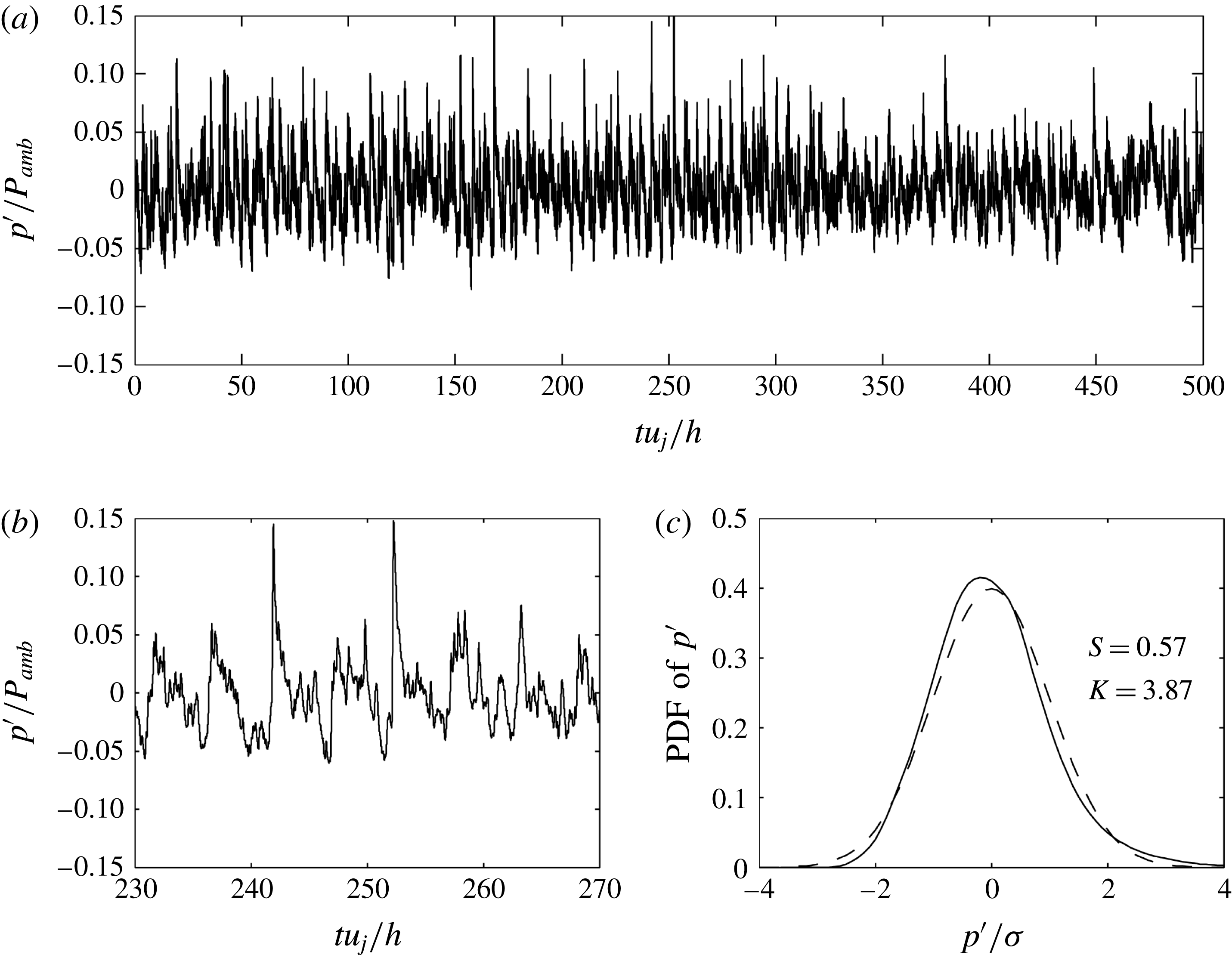
The nonlinear effects on the propagation of the acoustic waves generated by the jets are investigated by looking at the statistical properties of the pressure fluctuations at $x=0$ and $y=8.5h$ , at a distance far from the region of jet impingement in order to eventually obtain steep wave fronts. The skewness and the kurtosis factors calculated for the four jets are reported in table 4. Positive values of skewness between 0.27 and 0.57 are found. They appear to be higher when the peak level in the pressure spectra at $x=0$ and $y=1.5h$ , also provided in the table, increases. In particular, the strongest skewness and kurtosis values are reached for JetL5.5, which is also the most resonant case with a maximum sound level of $188~\text{dB}/St$ at $x=0$ and $y=1.5h$ .

Table 4.

Maximal levels in the sound spectra of figure 8, at $x=0$ and $y=1.5h$ , and skewness and kurtosis factors of the fluctuating pressure at $x=0$ and $y=8.5h$ .

For JetL5.5, in which the strongest resonance is obtained as mentioned above, the time variations of the pressure fluctuations recorded at $x=0$ and $y=8.5h$ are represented in figure 11(a) over the entire simulation time for $0\leqslant t\leqslant 500h/u_{j}$ , and in figure 11(b) for $230h/u_{j}\leqslant t\leqslant 270h/u_{j}$ . The probability density function of the full pressure signal is also shown in figure 11(c). Weak shock waves and $N$ -shaped waves with sharp compressions associated with gradual expansions are visible in figure 11(b). Similar observations were made by Baars & Tinney (Reference Baars and Tinney2013, Reference Baars and Tinney2014) in the acoustic field of a jet at Mach 3 and by de Cacqueray & Bogey (Reference de Cacqueray and Bogey2014) for an overexpanded jet at ${\mathcal{M}}_{j}=3.3$ . In addition, at certain times, the pressure fluctuations exceed 15 % of the ambient pressure. This is notably the case at $t=242h/u_{j}$ and $t=253h/u_{j}$ , where two strong shock waves are found. Finally, the skewness factor is equal to 0.57, and thus exceeds the value of 0.4 which indicates the probable presence of crackle noise according to Ffowcs-Williams, Simson & Virchis (Reference Ffowcs-Williams, Simson and Virchis1975).

Figure 11.

Pressure fluctuations at $x=0$ and $y=8.5h$ for JetL5.5: (a) time variations over the entire simulation, (b) variations over a short period and (c) —— probability density function and – – – probability density function of a Gaussian distribution where $\unicode[STIX]{x1D70E}$ represents the standard deviation of $p^{\prime }$ .

5.1 Fourier decomposition of the pressure field

In order to determine the amplitude and phase fields associated with the different tones of the feedback loop in the four jets, a Fourier transform in time is applied to the near pressure fields recorded every 50th LES time step in the $(x,y)$ plane. The results obtained for the dominant tone frequencies are represented in figure 12.

Figure 12.

Amplitude (a–d) and phase (e–h) fields obtained for the dominant tones in (a,e) JetL3.9 at $St=0.255$ , (b,f) JetL5.5 at $St=0.19$ , (c,g) JetL8.3 at $St=0.092$ and (d,h) JetL9.1 at $St=0.085$ .

The phase fields in the bottom views of figure 12 allow us to identify the nature of the oscillation modes associated with the tones. For JetL3.9 and JetL5.5, these modes are antisymmetric given the $180^{\circ }$ phase shift visible with respect to the jet axis in figure 12(e,f). For JetL8.3 and JetL9.1, on the contrary, they are symmetric since the phase is identical on both sides of the jet axis in figure 12(g,h). Symmetric and antisymmetric oscillation modes were also found experimentally by Norum (Reference Norum1991) at the tone frequencies of rectangular supersonic impinging jets.

The amplitude fields in the top views of figure 12 all exhibit a cell structure between the nozzle and the plate. By considering the two semi-cells near the nozzle and the plate as one cell, the cell structure appears to contain three cells for JetL3.9 and JetL5.5 in figure 12(a,b) and two cells for JetL8.3 and JetL9.1 in figure 12(c,d). Thus, at the dominant tone frequency, the number of cells is equal the mode number predicted by the model of Ho & Nosseir (Reference Ho and Nosseir1981), namely three for the two first jets and two for the others. Besides, it can be noted that the amplitude levels near the jet axis in figure 12(a,b) are very weak, as expected for antisymmetric oscillations.

The amplitude fields of figure 12 also provide information on the sound sources at the dominant tone frequencies. For JetL3.9, three acoustic components labelled (i), (ii) and (iii) are revealed by the spots of intense levels in figure 12(a). The first component can be seen on both sides of the jet for $0<\unicode[STIX]{x1D6FC}<20^{\circ }$ , where $\unicode[STIX]{x1D6FC}$ is the angle between the upstream direction and the propagation direction from the impingement region as illustrated in the figure. It is related to the upstream-propagating neutral acoustic waves of the jet, which will be further discussed later. The second acoustic component is visible for $30<\unicode[STIX]{x1D6FC}<50^{\circ }$ . It seems to propagate from a point around $x=2.5h$ and $y=1.5h$ , where strong pressure levels are found. Finally, the third acoustic component is noted for $\unicode[STIX]{x1D6FC}>60^{\circ }$ . It may be generated near the flat plate around $y=3h$ where, again, high pressure levels are obtained. For JetL5.5, two acoustic components can be observed in figure 12(b), for $0<\unicode[STIX]{x1D6FC}<30^{\circ }$ and for $\unicode[STIX]{x1D6FC}>40^{\circ }$ . As for JetL3.9, the first one may be due to the upstream-propagating neutral acoustic waves of the jet, and the second one may be produced near the plate around $y=3.5h$ . Finally, for JetL8.3 and JetL9.1, two acoustic contributions appear to similarly emerge.

5.2 Model of an hydrodynamic–acoustic standing wave

In self-sustaining oscillating flows, hydrodynamic–acoustic standing waves can be observed, as was the case in the screeching free supersonic jets of Panda et al. (Reference Panda, Raman and Zaman1997) and Panda & Seasholtz (Reference Panda and Seasholtz1999). These waves are due to the superposition of hydrodynamic waves propagating downstream and acoustic waves propagating upstream.

A simple model can be built to determine the wavenumber of the hydrodynamic–acoustic standing waves in the present jets. By denoting $\unicode[STIX]{x1D714}$ the angular frequency of the feedback mechanism, and $k_{p}$ and $k_{a}$ the wavenumbers of the hydrodynamic and acoustic waves, the fluctuating pressure in the jet shear layers can be written as

where $A_{a}$ , $A_{p}$ and $\unicode[STIX]{x1D719}_{a}$ and $\unicode[STIX]{x1D719}_{p}$ are the amplitudes and phase shifts of the acoustic and hydrodynamic waves. The quadratic mean value is then equal to

where $T=2\unicode[STIX]{x03C0}/\unicode[STIX]{x1D714}$ is the time period. Therefore, at the frequency of the feedback mechanism, the pattern of a standing wave with a wavenumber

is expected. By considering that $k_{sw}=2\unicode[STIX]{x03C0}/L_{sw}$ , $k_{p}=\unicode[STIX]{x1D714}/u_{c}$ and $k_{a}=\unicode[STIX]{x1D714}/a_{0}$ , where $L_{sw}$ is the wavelength of the hydrodynamic–acoustic standing wave, $u_{c}$ is the convection velocity in the jet shear layers and $a_{0}$ is the ambient speed of sound, one gets

where $f=2\unicode[STIX]{x03C0}/\unicode[STIX]{x1D714}$ . In the amplitude fields of figure 12, there is a whole number $N$ of cells between the nozzle lip and the flat plate. Assuming that the cell structures result from the presence of hydrodynamic–acoustic standing waves, this indicates that the nozzle-to-plate distance is a multiple of the wavelength $L_{sw}$ , that is $L=NL_{sw}$ , yielding

This equation is identical to (4.2) given by the model of Ho & Nosseir (Reference Ho and Nosseir1981), demonstrating that the number of cells in the standing wave is also the mode number. This result is consistent with the observations made in the previous section. The aeroacoustic feedback loop establishing between the nozzle and the plate thus leads to the formation of hydrodynamic–acoustic standing waves.

5.3 Wave analysis using a vortex sheet model of the jet

In the analytical study of small-amplitude waves in jets of Tam & Hu (Reference Tam and Hu1989), three families of instability waves were identified: the Kelvin–Helmholtz instability waves, which correspond to vorticity waves, and the supersonic and subsonic instability waves, which are acoustic waves (Berman & Williams Reference Berman and Williams1970; Mack Reference Mack1990; Sabatini & Bailly Reference Sabatini and Bailly2014). On the basis of this result, Tam & Norum (Reference Tam and Norum1992) suggested that the acoustic waves of the feedback loop in impinging jets are linked to the acoustic subsonic instability waves of the jets. These waves are found to be unstable for jets with mixing layers of finite thickness. For jets with mixing layers modelled by a vortex sheet (Tam & Hu Reference Tam and Hu1989), on the contrary, they are neutral, and have a real angular frequency, but also a real wavenumber.

In this work, as previously done by Tam & Norum (Reference Tam and Norum1992) for planar jets and Tam & Ahuja (Reference Tam and Ahuja1990) for round jets, a wave analysis is therefore carried out using a vortex sheet model in order to better describe the feedback loop in impinging jets. More precisely, the neutral acoustic waves of an ideally expanded 2-D jet of height $h$ , exit velocity $u_{j}$ and Mach number ${\mathcal{M}}_{j}$ , bounded by two vortex sheets, are investigated. A schematic representation of a symmetric instability of such a jet is provided in figure 13.

Figure 13.

Symmetric instability of a 2-D supersonic jet bounded by vortex sheets.

The pressure fluctuations, associated with small-amplitude disturbances superimposed on the mean flow inside and outside of the jet are denoted by $p_{int}$ and $p_{ext}$ , and the lateral displacement of the upper vortex sheet is given by $\unicode[STIX]{x1D701}(x,t)$ . The linearized continuity, momentum and energy equations for a compressible inviscid fluid

where $a_{0}$ and $a_{j}$ are the sound speeds in the ambient medium and in the jet, are considered. The boundary conditions on the upper vortex sheet located at $y=h/2$ are

where $\unicode[STIX]{x1D70C}_{0}$ are the densities in the ambient medium and in the jet. On the centreline, the boundary conditions for symmetric and antisymmetric modes are different, yielding

The equation system (5.6) being closed, wave solutions of the form

where $k$ and $\unicode[STIX]{x1D714}$ are the wavenumber and the angular frequency of the wave, can be sought. Two dispersion relations were found by Tam & Norum (Reference Tam and Norum1992). They are given by

for symmetric modes, and

for antisymmetric modes.

The solutions of the dispersion relations (5.10) and (5.11) calculated for the present jet are represented in figure 14 as functions of the Strouhal number and the wavenumber. Three symmetric neutral acoustic wave modes, referred to as $S1$ , $S2$ and $S3$ , appear in figure 14(a). In the same way, three antisymmetric modes denoted by $A1$ , $A2$ and $A3$ are found in figure 14(b).

Figure 14.

Dispersion relations for (a) the symmetric and (b) the antisymmetric neutral acoustic wave modes for an ideally expanded planar jet with ${\mathcal{M}}_{j}=1.28$ , ● lower limits of the modes, – – –  $k=-\unicode[STIX]{x1D714}/a_{0}$ .

According to Tam & Hu (Reference Tam and Hu1989), upstream-propagating acoustic waves are present in high-speed jets. They are confined in the jets when the jets are subsonic, but lie outside when the jets are supersonic. Such waves are found in figure 14 on the right-hand side of each mode where $\text{d}\,St/\text{d}k<0$ , leading to a negative group velocity $\text{d}\unicode[STIX]{x1D714}/\text{d}k$ . Allowable frequency ranges can thus be determined for the different modes. Their upper limits, which correspond to the maximum Strouhal numbers reached for the modes when $\text{d}\,St/\text{d}k=0$ , are obtained from the figure. Their lower limits are calculated, since they are necessarily associated with acoustic waves propagating with a group velocity of $-a_{0}$ , and located on the dashed line of figure 14 defined by

For $k=-\unicode[STIX]{x1D714}/a_{0}$ , the first terms in (5.10) and (5.11), and consequently the second terms, tend to infinity. The argument of the tangent function needs to be equal to

for (5.10) and

for (5.11), yielding the following Strouhal numbers for the lower limits of the allowable frequency ranges

for the symmetric modes and

for the antisymmetric modes, where $n$ is the mode number. The values calculated for the present jet are depicted in figure 14.

The allowable frequency ranges determined for the two first symmetric and antisymmetric upstream-propagating wave modes are represented in figure 15 as a function of the exit Mach number ${\mathcal{M}}_{j}$ . The dominant tone frequencies measured by Tam & Norum (Reference Tam and Norum1992) for cold rectangular impinging jets at Mach numbers between 1.15 and 1.70, for a large number of nozzle-to-plate distances in each case, are also shown. Two modes, namely a low-frequency symmetric mode and a high-frequency antisymmetric mode are observed in most cases. The dominant tone frequencies obtained for the four jets at ${\mathcal{M}}_{j}=1.28$ in the LES are also plotted in the figure. The tone frequencies for JetL3.9 and JetL5.5, at $St_{2}=0.255$ and $St_{2}=0.19$ , respectively, fall into the allowable range for the first symmetric mode, whereas the tone frequencies for JetL8.3 and JetL9.1, at $St_{1}=0.092$ and $St_{1}=0.085$ , lie in the allowable range for the first antisymmetric mode. Considering the results in § 5.2, the present wave analysis thus appears to predict the nature of the jet oscillation mode at the dominant tone frequencies, which is symmetric for the two first jets but antisymmetric for the two others. However, it only provides allowable frequency ranges. In order to better understand how, for a given nozzle-to-plate distance, discrete frequencies are selected over these ranges, this analysis is combined below with the aeroacoustic feedback model.

Figure 15.

Allowable frequency ranges for the upstream-propagating neutral acoustic wave modes as a function of the exit Mach number; symmetric modes are in light grey and antisymmetric modes are in dark grey; ● dominant tone frequencies in the experiments of Tam & Norum (Reference Tam and Norum1992) for rectangular supersonic cold jets and $\times$  dominant tone frequencies in the present LES.

5.4 Combination of the aeroacoustic feedback model and the wave analysis

The aeroacoustic feedback model and the wave analysis based on the vortex sheet model are combined in order to determine both the most likely possible tone frequencies of the feedback mechanism and the antisymmetric or symmetric nature of the corresponding modes. This is made possible by assuming that the acoustic wavenumber in the feedback loop is equal to the opposite of the wavenumber $k$ of the upstream propagating acoustic waves found in the wave analysis. Thus, the (5.3) relating the wavenumber $k_{sw}$ of the hydrodynamic–acoustic standing wave due to the feedback mechanism and the acoustic and hydrodynamic wavenumbers $k_{a}$ and $k_{p}$ leads to

given that $k_{sw}=2\unicode[STIX]{x03C0}N/L$ , $k_{p}=2\unicode[STIX]{x03C0}f/u_{c}$ and $k_{a}=-k$ . The feedback model and the wave analysis are then combined by representing this relation and the dispersion relations in the same figure for the different impinging jets. The results will be compared with the simulation results.

For JetL3.9, the phase and the amplitude fields obtained by LES for the three main tones at $St_{1}=0.115$ , $St_{2}=0.255$ and $St_{3}=0.37$ are displayed in figure 16. For $St_{1}=0.115$ , a $180^{\circ }$ phase shift with respect to the jet axis is found in the phase field of figure 16(b), indicating an antisymmetric oscillation mode. No cell structure clearly appears in the amplitude field of figure 16(a), suggesting the absence of an hydrodynamic–acoustic standing wave in this case. For $St_{2}=0.255$ , an antisymmetric oscillation mode is observed in figure 16(d), and a cell structure containing three cells between the nozzle and the plate is visible in figure 16(d). Finally, for $St_{3}=0.37$ , a symmetric oscillation mode and a cell structure with four cells are revealed by figure 16(e,f).

Figure 16.

Amplitude (a,c,e) and phase (b,d,f) fields obtained for the three dominant tones of JetL3.9 at $St_{1}=0.115$ , $St_{2}=0.255$ and $St_{3}=0.37$ , from left to right.

The results obtained for JetL3.9 by combining the feedback model and the wave analysis are represented in figure 17 by showing the dispersion relations of the acoustic wave modes for a planar jet at ${\mathcal{M}}_{j}=1.28$ together with the solutions of (5.17) for the first ten modes of the feedback mechanism, as functions of the Strouhal number and the wavenumber. The three dominant tones are also indicated on the line $k=-\unicode[STIX]{x1D714}/a_{0}$ , depending on the symmetric or antisymmetric nature of the corresponding oscillation modes. In figure 17(a), the tone at $St_{3}=0.37$ is found just below the symmetric mode $S2$ of the jet, on the line associated with the mode $N=4$ of the feedback loop. This is consistent with the results reported above for $St_{3}=0.37$ . In figure 17(b), the tone at $St_{2}=0.255$ is located at the intersection of the antisymmetric mode $A1$ of the jet and of the mode $N=3$ of the feedback loop. Again, this result is in agreement with the phase and amplitude fields provided by the LES. Finally, the tone at $St_{1}=0.115$ does not seem to be predicted by the model combination. It is not surprising given that $St_{1}$ is equal to $St_{3}-St_{2}$ , and that there is no hydrodynamic–acoustic standing wave in figure 16(a).

Figure 17.

Representation of —— the dispersion relations for (a) the symmetric and (b) the antisymmetric neutral acoustic wave modes for an ideally expanded planar jet with ${\mathcal{M}}_{j}=1.28$ , ● lower limits of the modes, – – –  $k=-\unicode[STIX]{x1D714}/a_{0}$ , 

 relation (5.17) for $L=3.94h$ , * dominant tone frequencies of JetL3.9.

The phase and the amplitude fields obtained for JetL5.5 at the two main tone frequencies at $St_{1}=0.12$ and $St_{2}=0.19$ are displayed in figure 18. The phase fields indicate a symmetric oscillation mode for the first tone and an antisymmetric oscillation mode for the second one. Moreover, cell structures containing two and three cells, respectively, between the nozzle and the plate appear in the amplitude fields.

Figure 18.

Amplitude (a,c) and phase (b,d) fields obtained for the two dominant tones of JetL5.5 at $St_{1}=0.12$ and $St_{2}=0.19$ , from left to right.

The results of the model combination for JetL5.5 are shown in figure 19, in which the two dominant tones obtained in the LES for this jet are also represented. In figure 19(a), the tone at $St_{1}=0.12$ lies at the intersection of the symmetric mode $S1$ of the jet and of the second mode of the feedback loop, which is in agreement with the tone properties observed in figure 18(a,b). In figure 19(b), the tone at $St_{2}=0.19$ is located very near the antisymmetric mode $A1$ of the jet and on the third mode of the feedback loop, which is also in line with the amplitude and phase fields of figure 18(c,d).

Figure 19.

Representation of —— the dispersion relations for (a) the symmetric and (b) the antisymmetric neutral acoustic wave modes for an ideally expanded planar jet with ${\mathcal{M}}_{j}=1.28$ , ● lower limits of the modes, – – –  $k=-\unicode[STIX]{x1D714}/a_{0}$ , 

 relation (5.17) for $L=5.5h$ , * dominant tone frequencies of JetL5.5.

The phase and amplitude fields obtained for JetL8.3 at the four main tone frequencies, at $St_{1}=0.092$ , $St_{2}=0.165$ , $St_{3}=0.21$ and $St_{4}=0.255$ are given in figure 20. For the first tone, a symmetric oscillation mode and a cell structure containing two cells are seen in figure 20(a,b). For the three other tones, antisymmetric oscillation modes and cell structures containing four, five and six cells, respectively, are noted in figure 20(c–h).

Figure 20.

Amplitude (a,c,e,g) and phase (b,d,f,h) fields obtained for the four dominant tones of JetL8.3 (a–d) at $St_{1}=0.092$ and $St_{2}=0.165$ , and (e–h) at $St_{3}=0.21$ and $St_{4}=0.255$ , from left to right.

The results of the model combination for JetL8.3 and the four dominant tones in this jet are displayed in figure 19. In figure 21(a), the first tone at $St_{1}=0.092$ is very close to the intersection of the symmetric jet mode  $S1$ and the second mode of the feedback loop. In figure 21(b), the second, third and fourth tones are found near or on the antisymmetric mode  $A1$ of the jet and on the fourth, fifth and sixth modes of the feedback loop, respectively. These findings are consistent with the amplitude and phase fields of figure 20.

Figure 21.

Representation of —— the dispersion relations for (a) the symmetric and (b) the antisymmetric neutral acoustic wave modes for an ideally expanded planar jet with ${\mathcal{M}}_{j}=1.28$ , ● lower limits of the modes, – – –  $k=-\unicode[STIX]{x1D714}/a_{0}$ , 

 relation (5.17) for $L=8.27h$ , * dominant tone frequencies of JetL8.3.

For brevity, the amplitude and phase fields obtained for JetL9.1 at the four main tone frequencies and the results given by the model combination in this case are not presented, because they are very similar to those reported above for JetL8.3.

In summary, the proposed model combination applies successfully to the present impinging jets. The tone frequencies obtained in the LES lie near the lower limits of the allowable ranges predicted by the wave analysis for the upstream-propagating acoustic wave modes. This trend can be due to the fact that, in the vicinity of the lower limits of the modes, the group velocity of the neutral acoustic waves is very close to $-a_{0}$ . Consequently, these waves are the most likely to sustain an acoustic feedback. Having noted this, it seems possible to predict the most probable tones, their frequencies and their symmetric or antisymmetric natures. For the antisymmetric modes, the tone frequencies can be expected to be located near the lower limit of the mode  $A1$ , as is the case for the four jets of this study. For the symmetric modes, they can be found near the lower limit of the mode  $S2$ , as for JetL3.9, but also at the intersections between the modes  $S1$ and the different modes of the feedback loop, as for the other jets. Obtaining a tone frequency at the first intersection point between the mode  $S1$ and the mode $N=1$ of the feedback loop is however unlikely given the very low Strouhal number $St<0.05$ at this point.

Finally, note that a similar wave analysis can be performed for jets with mixing layers of finite thickness, as in Tam & Ahuja (Reference Tam and Ahuja1990). In this case, the frequencies of the lower limits of the allowable bands for the upstream-propagating acoustic wave modes are lower than using the vortex sheet model. This could explain why tone frequencies are found just below the lower limits of allowable bands for JetL3.9, JetL8.3 and JetL9.1 in the present study.