2.1. Governing equation

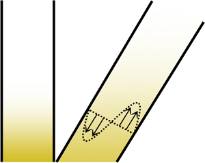
Figure 1 sketches two coordinate systems for a tilted parallel-plate channel domain with an inclination angle $\theta$ relative to the horizontal plane, which satisfies $0\leq \theta \leq {{\rm \pi} }/{2}$. In this set-up, the $x_3$-direction is parallel to the direction of gravity. Here $\varOmega =\{ y_{3}| y_3 \in [0,H] \}$ is the cross-section of the channel, where $H$ is the distance between plates. The longitudinal direction of the channel is denoted as the $y_1$-direction, with $y_{1}\in [-L,L]$, where $L$ may be either infinite or a finite number that is significantly larger than $H$. The relation between the laboratory frame coordinates $(x_{1},x_{2},x_{3})$ and the coordinates $(y_{1},y_{2},y_{3})$ is

(2.1)\begin{equation} \begin{bmatrix} y_{1}\\ y_{3}\\ \end{bmatrix} = \begin{bmatrix} \cos \theta & \sin \theta \\ -\sin \theta & \cos \theta\\ \end{bmatrix} \begin{bmatrix} x_{1}\\ x_{3}\\ \end{bmatrix}, \quad y_{2}=x_{2}. \end{equation}

In the $(y_{1},y_{2},y_{3})$ coordinate system, gravity acts along the direction $(-\sin \theta, 0, -\cos \theta )$. Experimental methods described in Allshouse (Reference Allshouse2010) and Heitz et al. (Reference Heitz, Peacock and Stocker2005) provide feasible set-ups for this study. Another promising experimental configuration involves using temperature-stratified liquid gallium (Braunsfurth et al. Reference Braunsfurth, Skeldon, Juel, Mullin and Riley1997).

Figure 1.

This schematic illustrates the set-up for the diffusion-driven flow problem. Tilted impermeable boundaries induce the diffusion-driven flow, while there is no flow in the vertically oriented channel ($\theta ={{\rm \pi} }/{2}$). Pure molecular diffusion governs the scalar distribution in the latter case. As depicted in (a), at $t=0$, the concentration profiles are approximately the same in both channels. However, as time progresses, the dispersion of the scalar becomes more pronounced in the tilted channel compared with the vertically oriented one. In addition, the flow strength decreases as the density gradient decreases.

We consider a scalar $c$ responsible for fluid density stratification, referred to as the stratified scalar in the subsequent context, such as temperature or solute concentration. The density is assumed to be a specified function of the stratified scalar. For example, Abaid et al. (Reference Abaid, Adalsteinsson, Agyapong and McLaughlin2004) obtained the formula for the density of a sodium chloride solution as $\rho = 0.9971 + 0.00065S + 0.000322(25-T)\ {\rm g}\ {\rm cm}^{-3}$, where salinity $S$ is measured in parts per thousand and temperature $T$ is in degrees Celsius. In cases with a broader range of salinity, the relationship may exhibit nonlinearity. Hall (Reference Hall1924), through empirical data fitting, established $\rho =0.997071+0.00070109 S+ 1.3268\times 10^{-7}S^{2}+3.535\times 10^{-10} S^3 \ {\rm g}\ {\rm cm}^{-3}$ for sodium chloride solutions at $25\,^{\circ}$C. The theoretical method presented in this work can be easily extended to cases with variable fluid viscosity. However, for simplicity, we assume the fluid dynamic viscosity is constant throughout the paper.

The stratified scalar $c$ and the fluid flow $\boldsymbol {u}=(u_{1},u_{2},u_{3})$ in the $\boldsymbol {x}= (x_{1},x_{2},x_{3})$ direction satisfy the incompressible Navier–Stokes equation,

(2.2)\begin{align} \left.\begin{array}{c} \rho (c) ( \partial_{t} u_{i}+ \boldsymbol{u}\boldsymbol{\cdot} \boldsymbol{\nabla} u_{i} ) = \mu \Delta u_{i} - \partial_{x_{i}} p- \rho (c) g \delta_{i3},\quad u_{i} |_{\boldsymbol{x}\in \partial \varOmega}=0,\quad i=1,2,3,\\ \boldsymbol{\nabla} \boldsymbol{\cdot} \boldsymbol{u}=0,\quad \partial_{t}c+ \boldsymbol{u}\boldsymbol{\cdot} \boldsymbol{\nabla} c= \kappa \Delta c,\quad \partial_{\boldsymbol{n}}c |_{\boldsymbol{x}\in\partial \varOmega }=0, \quad c|_{t=0}=c_{I}(\boldsymbol{x}), \end{array}\right\} \end{align}

where $\boldsymbol {n}$ is the outward normal vector of the boundary, $\delta _{ij}$ is the Kronecker delta, $g$ (cm s$^{-2}$) is the acceleration of gravity, $\rho$ (g cm$^{-3})$ is the density, $\mu$ (g cm$^{-1}$ s$^{-1})$ is the dynamic viscosity, $p$ (g cm$^{-1}$ s$^{-2})$ is the pressure and $\kappa$ (cm$^{2}$ s$^{-1})$ is the molecular diffusivity of the stratified scalar.

It is convenient to consider the problem in the $(y_{1},y_{2},y_{3})$ coordinate system. We denote $v_i$ as the velocity component along the $y_{i}$-direction. Since the initial condition and the boundary condition are independent of $y_2$, (2.2) reduces to a two-dimensional problem

(2.3)\begin{equation} \left.\begin{array}{c} \rho ( \partial_{t} v_{1}+ v_{1}\partial_{y_{1}} v_{1} + v_{3}\partial_{y_{3}} v_{1}) =\mu \Delta v_{1} - \partial_{y_{1}} p- \sin \theta g \rho ,\\ \rho ( \partial_{t} v_{3}+ v_{1}\partial_{y_{1}} v_{3} + v_{3}\partial_{y_{3}} v_{3}) =\mu \Delta v_{3} - \partial_{y_{3}} p- \cos \theta g\rho ,\\ \partial_{t}c+ \boldsymbol{v} \boldsymbol{\cdot} \boldsymbol{\nabla} c= \kappa \Delta c, \quad \boldsymbol{\nabla} \boldsymbol{\cdot} \boldsymbol{v}=0,\quad \boldsymbol{v} |_{\boldsymbol{y}\in \partial \varOmega }=\boldsymbol{0}, \quad \partial_{\boldsymbol{n}}c |_{\boldsymbol{y}\in\partial \varOmega}=0. \end{array} \right\} \end{equation}

In this study, we assume the initial density profile is a stable density stratification, where the density decreases monotonically as the height increases, namely, $\partial _{y_{1}}\rho (\bar {c}_{I}) \leq 0$. For convenience, we use the overline to represent the cross-sectional average of a quantity and use the tilde to represent the fluctuation, for example, $\overline {c_{I}}(y_{1})= \int _0^1 c_{I}(y_{1},y_{3}) \,\mathrm {d} y_{3}$.

2.2. Non-dimensionalization

As the flow is driven by molecular diffusion, we select the diffusion time scale as the characteristic time, ${H^{2}}/{\kappa }$. Specifically, it refers to the time it takes for solute molecules to diffuse across the cross-sectional area of the channel domain. Utilizing the following change of variables for non-dimensionalization:

(2.4)\begin{equation} \rho_{0}\rho'=\rho , \quad c_{0}c'=c, \quad\frac{H^2}{\kappa} t' =t, \quad H\boldsymbol{y}'=\boldsymbol{y}, \quad U\boldsymbol{v}'=\boldsymbol{v}, \quad \frac{\mu U}{H} p' =p, \end{equation}

then (2.3) becomes

(2.5) \begin{align} \left.\begin{array}{c} \displaystyle \rho' \left( \dfrac{U \kappa}{H^2} \partial_{t'} v_{1}'+ \dfrac{U^{2}}{H} v_{1}'\partial_{y_{1}'} v_{1}' + \dfrac{U^{2}}{H} v_{3}'\partial_{y_{3}'} v_{1}'\right) =\dfrac{ \mu U}{H^2\rho_{0}} \varDelta_{\boldsymbol{y}'} v_{1}' - \dfrac{\mu U}{H^2\rho_{0}}\partial_{y_{1}'} p'- \sin \theta g \rho' , \\ \displaystyle \rho' \left( \dfrac{U \kappa}{H^2} \partial_{t'} v_{3}'+ \dfrac{U^{2}}{H} v_{1}'\partial_{y_{1}'} v_{3}' +\dfrac{U^{2}}{H} v_{3}'\partial_{y_{3}'} v_{3}'\right) =\dfrac{ \mu U}{H^2\rho_{0}} \varDelta_{\boldsymbol{y}'} v_{3}' - \dfrac{\mu U}{H^2\rho_{0}}\partial_{y_{3}'} p'- \cos \theta g\rho' , \\ \displaystyle \dfrac{c_0\kappa}{H^2} \partial_{t'}c'+ \dfrac{U c_{0}}{H} \boldsymbol{v}' \boldsymbol{\cdot} \boldsymbol{\nabla} _{\boldsymbol{y}'}c'= \dfrac{\kappa c_{0}}{H^2} \varDelta_{\boldsymbol{y}'}c',\quad \dfrac{c_{0}}{H} \partial_{\boldsymbol{n}'}c' |_{\boldsymbol{y}'\in \partial \varOmega'}=0. \end{array} \right\} \end{align}

We can drop the primes without confusion and obtain the non-dimensionalized version

(2.6)\begin{align} \left.\begin{array}{c} \displaystyle \rho \left( \dfrac{1}{Sc} \partial_{t} v_{1}+ {Re} v_{1}\partial_{y_{1}} v_{1} + {Re} v_{3}\partial_{y_{3}} v_{1}\right) =\Delta v_{1} - \partial_{y_{1}} p- {Re}\, {Ri}\rho \sin \theta, \\ \displaystyle \rho \left( \dfrac{1}{Sc} \partial_{t} v_{3}+ {Re} v_{1}\partial_{y_{1}} v_{3} +{Re} v_{3}\partial_{y_{3}} v_{3}\right) = \Delta v_{3} - \partial_{y_{3}} p- {Re}\, {Ri}\rho \cos \theta, \\ \partial_{t}c+ {Pe} \boldsymbol{v} \boldsymbol{\cdot} \boldsymbol{\nabla} c= \Delta c, \end{array} \right\} \end{align}

where the non-dimensional parameters are Péclet number ${Pe}= {UH}/{\kappa }$, Reynolds number ${Re}= {\rho _{0} H U}/{\mu }$, Richardson number ${Ri}= {g H}/{U^{2}}$ and Schmidt number ${Sc}= {\mu }/{\rho _{0} \kappa }={Pe}/{Re}$. If the scalar field is the temperature field, then $\kappa$ is the thermal diffusivity and ${Pr}={\mu }/{\rho _{0} \kappa }={Pe}/{Re}$ is the Prandtl number.

We proceed by examining a combination of experimental physical parameters, which can provide us with the order of magnitude of the non-dimensional parameters and assist in our perturbation analysis. The previous experiments primarily focused on diffusion in linearly stratified fluids. It is feasible to adapt these set-ups for experiments involving nonlinearly stratified fluids, making the parameters therein useful as reference points. For instance, in Camassa et al. (Reference Camassa, Harris, Hunt, Kilic and McLaughlin2019), a linear density stratification of the fluid was achieved using sodium chloride. The relevant physical parameters in this context are as follows: $g=980\ \textrm {cm}\ \textrm {s}^{-2}$, $\mu _{0}=0.008903\ \textrm {g}\ (\textrm {cm}~\textrm {s})^{-1}$, $\kappa = 1.5\times 10^{-5}\ \textrm {cm}^{2}\ \textrm {s}^{-1}$ (Vitagliano & Lyons Reference Vitagliano and Lyons1956), $\rho _{0}= 0.9971\ \textrm {g}\ \textrm {cm}^{-3}$, the vertical density gradient $\partial _{x_{3}}\rho$ is a constant $0.007\ \textrm {g}\ \textrm {cm}^{-4}$. The scaling relation for the characteristic velocity and the physical parameters varies depending on the boundary geometries. For a linear stratified fluid, the characteristic velocity and characteristic boundary layer thickness of steady diffusion-driven flow in a parallel-plate channel can be calculated using the formula from (Phillips Reference Phillips1970; Heitz et al. Reference Heitz, Peacock and Stocker2005) as follows:

(2.7a,b)\begin{equation} U =2 \kappa \cot (\theta ) \left( \frac{ g \sin (\theta) \partial_{x_{3}}\rho}{4 \kappa \mu } \right)^{{1}/{4}},\quad H_{b}=\left( \frac{ g \sin (\theta )\partial_{x_{3}}\rho }{4 \kappa \mu } \right)^{-{1}/{4}}. \end{equation}

Using these formulae, we obtain the values $U =0.00164684\ \textrm {cm}\ \textrm {s}^{-1}$, $H_{b}= 0.0182167$ cm for $\theta ={{\rm \pi} }/{4}$. When the gap thickness between two walls is $H=0.1$ cm, this leads to the following non-dimensional parameters:

(2.8a––d)\begin{equation} {Re}=0.0184512,\quad {Pe}=10.9799, \quad {Sc}=595.076, \quad {Re} \, {Ri}=666613. \end{equation}

It is evident that the Reynolds number is small, indicating that viscous effects dominate the flow, and the gravity term is significant in the governing equation.

Last, with the above parameters and $c_{0}=1\ \textrm {mol}\ \textrm {kg}^{-1}$, the relation between $\rho$ and $c$ can be expressed as

(2.9)\begin{equation} \rho (c)=1+0.0410921 c+ 0.000454464 c^2+ 0.000070761 c^3. \end{equation}

3.1. Expansions for slow varying density profile

To address the scenario where the longitudinal length scale of the channel domain significantly exceeds the transverse length scale, our objective is to develop a simplified model that relies solely on the longitudinal variable of the channel domain. To achieve this, we adopt the following ansatz for the velocity and density:

(3.3) \begin{align} \left.\begin{array}{c}\!\! v_{1} (y_{1},y_{3},t) =v_{1,0}(y_{3},t, \bar{c})+v_{1,1} (y_{3},t, \partial_{y_{1}}\bar{c} )\partial_{y_{1}}\bar{c}+v_{1,2} (y_{3},t, \partial_{y_{1}}\bar{c},\partial_{y_{1}}^{2}\bar{c} ) \partial_{y_{1}}^{2}\bar{c}+\cdots, \\ \!\! v_{3}(y_{1},y_{3},t)=v_{3,0}(y_{3},t,\bar{c})+v_{3,1} (y_{3},t, \partial_{y_{1}}\bar{c} )\partial_{y_{1}}\bar{c}+v_{3,2} (\kern0.08em y_{3},t, \partial_{y_{1}}\bar{c},\partial_{y_{1}}^{2}\bar{c} ) \partial_{y_{1}}^{2}\bar{c}+\cdots, \\ \!\! c(y_{1},y_{3},t)=\bar{c}(y_{1},t)+ c_{1} (y_{3},t, \partial_{y_{1}}\bar{c} )\partial_{y_{1}}\bar{c}+c_{2} (\kern0.08em y_{3},t, \partial_{y_{1}}\bar{c},\partial_{y_{1}}^{2}\bar{c} ) \partial_{y_{1}}^{2}\bar{c}+\cdots,\\ \!\! p(y_{1},y_{3},t)=p_{0}(y_{1},y_{3},t)+ p_{1} (y_{3},t, \partial_{y_{1}}\bar{c} )\partial_{y_{1}}\bar{c}+p_{2} (\kern0.08em y_{3},t, \partial_{y_{1}}\bar{c},\partial_{y_{1}}^{2}\bar{c} ) \partial_{y_{1}}^{2}\bar{c}+\cdots. \end{array}\!\!\! \right\} \end{align}

In this expansion, $v_{i,1},c_{1},p_{1}$ are functions of $\partial _{y_{1}}\bar {c}$. Here $v_{j,2},c_{2},p_{2}$ are functions of $\partial _{y_{1}}\bar {c}$ and $\partial _{y_{1}}^{2}\bar {c}$. The $j$th term in the expansion is contingent on the derivative of $\bar {c}$ up to the $j$th order. By definition, $\partial _{y_{1}}\bar {c}$ is independent of $y_{3}$ and is solely a function of $y_{1}$ and $t$. For the specific problem we investigate here, both $v_{i,j}$ and $c_{i}$ are functions of $y_{3}$ and $t$, while their dependence on $y_{1}$ is captured through $\partial _{y_{1}}\bar {c}$. In more general cases, such as the domain with non-flat boundary, $v_{i,j}$ and $c_{i}$ may depend on $y_{1}$.

In our analysis, we consider the derivative of the averaged stratified scalar, $\partial _{y_{1}}^{n}\bar {c}$, as a small parameter within the framework of standard asymptotic calculations. Additionally, we assume that higher-order derivatives exhibit smaller magnitudes compared with lower-order derivatives. This assumption is reasonable for systems where diffusion dominates.

To provide an intuitive justification, we assume that flow effects are negligible, and diffusion is the dominant process in the system. Under these conditions, the scalar field exhibits a self-similarity solution represented as $\bar {c} = \frac {1}{2} \textrm {erfc}({y_{1}}/{2 \sqrt {t}})$, where $\mathrm {erfc}(z) = ({2}/{\sqrt {{\rm \pi} }})\int _z^\infty \textrm {e}^{-t^2} \, \textrm {d} t$. The derivatives of this solution are as follows:

(3.4)\begin{align} \left.\begin{array}{c} \displaystyle \partial_{y_{1}}\bar{c} ={-}\dfrac{{\rm e}^{-{y_{1}^2}/{4 t}}}{2 \sqrt{\rm \pi} \sqrt{t}},\quad \partial_{y_{1}}^{2}\bar{c} ={-} \dfrac{y_{1}\, {\rm e}^{-{y_{1}^2}/{4 t}}}{4 \sqrt{\rm \pi} t^{3/2}},\\ \displaystyle \partial_{y_{1}}^{n}\bar{c}={-}\dfrac{1}{\sqrt{{\rm \pi} }}\left(-\dfrac{1}{2 \sqrt{t}}\right)^n H_{n-1}\left(\dfrac{y_{1}}{2 \sqrt{t}}\right) {\rm e}^{-(\kern0.08em {y_{1}}/{2 \sqrt{t}})^2}, \end{array} \right\} \end{align}

where $H_{n}$ is the Hermite polynomial of degree $n$. In general, as $t$ approaches infinity, we have $\partial _{y_{1}}^{n}\bar {c} = O(t^{-n+{1}/{2}})$. Consequently, as $t\rightarrow \infty$, we observe the hierarchy $\bar {c} \gg \partial _{y_{1}}\bar {c} \gg \partial _{y_{1}}^{2}\bar {c} \gg \cdots$. Due to the orthogonality of the Hermite polynomial, $\partial _{y_{1}}^{n}\bar {c}$ forms a good basis for approximating the function. In addition, it is important to note that in the presence of a diffusion-driven flow, as we will demonstrate in the following sections, the scaling relationship can differ. For instance, in some parameter limit, the self-similarity variable in the solution can be $y_{1}t^{-{1}/{4}}$ for finite $t$. However, in this case, the derivatives of the averaged density still tend to be zero, and the higher-order derivatives become much smaller than the lower-order derivatives as $t\rightarrow \infty$.

The similar form of expansion (3.3) has found applications in various fields, including the modelling of chromatograph and reactors (Balakotaiah, Chang & Smith Reference Balakotaiah, Chang and Smith1995), thin film fluid flows (Van Dyke Reference Van Dyke1987; Roberts Reference Roberts1996; Roberts & Li Reference Roberts and Li2006) and shear dispersion of passive scalars (Gill Reference Gill1967; Mercer & Roberts Reference Mercer and Roberts1990; Young & Jones Reference Young and Jones1991; Ding & McLaughlin Reference Ding and McLaughlin2022a). A more rigorous foundation for this expansion can be established through centre manifold theory (Carr Reference Carr1979; Roberts Reference Roberts1988, Reference Roberts2014, Reference Roberts2015; Aulbach & Wanner Reference Aulbach and Wanner1996, Reference Aulbach and Wanner1999). For in-depth discussions on constructing centre manifolds, we refer interested readers to the cited literature, and we will not delve into the details here.

Another possible asymptotic expansion approach is a power series expansion involving a small parameter, denoted as $\epsilon$, such as $c = \sum _{i=0}^{\infty }c_{i}\epsilon ^{i}$. This approach is commonly used in multiscale analysis (Kondic Reference Kondic2003; Pavliotis & Stuart Reference Pavliotis and Stuart2008; Wu & Chen Reference Wu and Chen2014; Ding Reference Ding2023). In this context, we highlight two advantages of the ansatz provided by (3.3) over the classical power series expansion for the specific problem addressed in this study.

First, in the classical ansatz, the coefficients remain independent of the small parameter $\epsilon$. The quantity is expanded as a linear combination of $\epsilon$ powers. In contrast, in (3.3), the coefficients depend on small quantities, namely, the derivatives of the averaged scalar field. This nonlinear dependency enables us to achieve a more accurate approximation using fewer terms.

Second, when applying the standard multiscale analysis method to this problem, the results depend on the scaling relation between parameters. In the thin film limit, as we will discuss in § 5, the scalar field can be approximated as $c=c_{0} (y_{1},t) +\epsilon c_{2}(y_{1},y_{3},t)$, where $c_{0}$ is the solution to a diffusion equation with a diffusivity of unity. In this scaling relation, the diffusion process is dominant, and the diffusion-driven flow does not have a first-order contribution. For cases where the diffusion-driven flow significantly enhances the dispersion of the stratified agent, an asymptotic analysis using a different scaling relation for physical parameters become necessary. In some cases, selecting the most appropriate characteristic parameter can be challenging. Additionally, since certain scales in the problem are time-dependent, the choice of scale may lead to time-dependent small parameters, which can complicate the development of a model that is uniformly valid across a wide range of parameter regimes.

In § 5, we will provide detailed explanations of the thin film approximation and discuss the differences between these two approaches.

3.2. Leading-order term in asymptotic expansion

The expansion (3.3) suggests that the deviation of the stratified scalar from its cross-sectional average is small. Consequently, this motivates us to examine the evolution equation for the cross-sectional averaged stratified scalar $\bar {c}$. Taking the cross-sectional average on both sides of the advection–diffusion equation (3.2) and utilizing the incompressibility condition and non-flux boundary condition yields

(3.5)\begin{equation} \partial_{t} \bar{c}+ {Pe}\partial_{y_{1}} \overline{v_{1}c}= \partial_{y_{1}}^{2}\bar{c}. \end{equation}

Therefore, to obtain the leading-order approximation for the cross-sectional averaged stratified scalar, we need to compute $v_{1,0}$, $v_{1,1}$ and $c_{1}$ in the expansion (3.3).

There are some observations that can simplify the calculation of asymptotic expansion. Since the flow is induced via the density gradient, the fluid flow vanishes as $\partial _{y_{1}}\bar {c}$ vanishes. Therefore, $v_{1,0}=v_{3,0}=0$. Substituting the expansion (3.3) into the continuity equation and noticing that $\partial _{y_{1}} ( v_{1,1}\partial _{y_{1}}\bar {c} )= O( \partial _{y_{1}}^{2} \bar {c})$, we obtain

(3.6)\begin{equation} \partial_{y_{1}}v_{1,0}+ \partial_{y_{3}}v_{3,1}=0. \end{equation}

Then to satisfy the no-slip boundary condition, $v_{3,1}$ must be zero.

Collecting the terms that are comparable to $\partial _{y_{1}}\bar {c}$ yields the following equation:

(3.7)\begin{equation} \left.\begin{array}{c} \displaystyle \dfrac{1}{Sc}\rho(\bar{c})\partial_{t}v_{1,1}= \partial_{y_{3}}^2v_{1,1}- {Re}\, {Ri} \partial_{c}\rho (\bar{c}) \left( c_{1} \sin \theta -\cos \theta\left(y_{3}-\dfrac{1}{2}\right)\right),\\ \partial_{t}c_{1}+ {Pe} v_{1,1} \partial_{y_{1}}\bar{c}=\partial_{y_{3}}^{2} c_{1}, \quad \partial_{y_3}c_{1}|_{y_{3}=0,1 }=0,\quad v_{1,1}|_{y_{3}=0,1 }=0. \end{array} \right\} \end{equation}

Previous studies (Kistovich & Chashechkin Reference Kistovich and Chashechkin1993; Ding & McLaughlin Reference Ding and McLaughlin2023) have uncovered fascinating dynamics in the time-dependent solution, particularly during short time scales when the initial velocity field is zero. However, these transient dynamics decay exponentially, and the solution converges to a steady-state either at the diffusion time scale or the viscosity time scale, depending on which of the two is larger. In many cases, the diffusion time scale significantly exceeds or is comparable to the viscosity time scale. For instance, in solute–liquid systems, the diffusivity of the solute molecule typically falls within the range of $10^{-5}\ \textrm {cm}^{2}\ \textrm {s}^{-1}$, while the kinematic viscosity of the liquid is around $10^{-2}\ \textrm {cm}^{2}\ \textrm {s}^{-1}$, resulting in a Schmidt number (${Sc}$) of $10^{3}$. In the case of temperature-stratified systems, the thermal diffusivity typically registers at approximately $10^{-3}\ \textrm {cm}^{2}\ \textrm {s}^{-1}$, with ${Pr}=10$. In both cases, the diffusion time scale is much larger than the viscosity time scale. Therefore, given our specific interest in approximations at the diffusion time scale and to streamline our analysis without compromising accuracy, our primary focus will be on the steady-state solution of the aforementioned equation. By neglecting the time derivatives in (3.7), we arrive at the following non-homogeneous linear system for analysis:

(3.8)\begin{equation} \left.\begin{array}{c} 0= \partial_{y_{3}}^2v_{1,1}- {Re}\, {Ri}\partial_{c}\rho (\bar{c}) (\sin \theta c_{1} -\cos \theta (y_{3}-\tfrac{1}{2})), \quad v_{1,1} |_{y_{3}=0,1 }=0, \\ {Pe} v_{1,1} \partial_{y_{1}}\bar{c}=\partial_{y_{3}}^{2} c_{1}, \quad \partial_{y_3}c_{1} |_{y_{3}=0,1 }=0. \end{array} \right\} \end{equation}

Differencing the above equation twice with respect to $y_{3}$ yields

(3.9)\begin{equation} \left.\begin{array}{c} 0= \partial_{y_{3}}^4v_{1,1}- {Re}\, {Ri} \sin \theta \partial_{c}\rho \partial_{y_{3}}^{2} c_{1}, \quad {Pe} \partial_{y_{1}}\bar{c} \partial_{y_{3}}^{2}v_{1,1}=\partial_{y_{3}}^{4} c_{1}, \\ \partial_{y_{3}}^{3}v_{1,1} |_{y_{3}=0,1 }={-}{Re}\, {Ri} \partial_{c}\rho (\bar{c}) \cos \theta. \end{array}\right\} \end{equation}

Then we can decouple the scalar field and velocity as

(3.10)\begin{equation} \left.\begin{array}{c} 0=\partial_{y_{3}}^4v_{1,1} -{Re}\,{Pe}\,{Ri}\sin \theta \partial_{y_{1}}\rho(\bar{c}) v_{1,1}, \quad v_{1,1} |_{y_{3}=0,1 }=0,\\ \partial_{y_{3}}^{3}v_{1,1} |_{y_{3}=0,1 }={-}{Re}\,{Ri} \partial_{c}\rho (\bar{c}) \cos \theta, \\ \partial_{y_{3}}^{4} c_{1}= {Re}\,{Pe}\,{Ri} \partial_{y_{1}}\rho(\bar{c}) ( \sin \theta c_{1} -\cos \theta(y_{3}-\tfrac{1}{2}) ) , \\ \partial_{y_3}c_{1} |_{y_{3}=0,1 }=0, \quad \partial_{y_2}^{2}c_{1} |_{y_{3}=0,1 }=0, \end{array} \right\} \end{equation}

where we have used $\partial _{y_{1}}\rho (\bar {c})=\partial _{c}\rho (\bar {c}) \partial _{y_{1}} \bar {c}$ to simplify the equation. We can solve the equation and express $v_{1,1}$, $c_{1}$ in terms of $\partial _{y_{1}}\bar {c}$ as follows:

(3.11) \begin{align} \left.\begin{array}{c} \displaystyle v_{1,1}= \dfrac{2 \gamma \cot (\theta )}{{Pe}\partial_{y_{1}} \bar{c}} \dfrac{ \sin (\gamma y_{3}) \sinh (\gamma (1- y_{3}))-\sin (\gamma (1- y_{3})) \sinh (\gamma y_{3}) }{ \sin (\gamma )+\sinh (\gamma )},\\ \displaystyle c_{1}=\cot \theta \left( y_{3}- \dfrac{1}{2}-\dfrac{ \cos (\gamma(1- y_{3})) \cosh (\gamma y_{3})-\cos (\gamma y_{3}) \cosh (\gamma(1- y_{3}))}{\gamma (\sin (\gamma)+\sinh (\gamma))} \right), \end{array} \right\} \end{align}

where $\gamma = ({1}/{\sqrt {2}})( -{Re}\, {Pe} \,{Ri} \sin \theta \partial _{y_{1}}\rho (\bar {c}))^{{1}/{4}}$. Recall our assumption of the stable density stratification, $\partial _{y_{1}}\rho (\bar {c})\leq 0$, which implies that $\gamma$ is a real non-negative number. In the case of linear density stratification, the equation above aligns with the steady solution previously presented in Phillips (Reference Phillips1970) and Heitz et al. (Reference Heitz, Peacock and Stocker2005).

As depicted in figure 2, both the normalized velocity $v_{1} \gamma ^{-1}\approx v_{1,1}\partial _{y_{1}}\bar {c}\gamma ^{-1}$ and $c_{1}$ are tightly confined within a narrow region near the boundary, especially when $\gamma$ is large. The velocity is positive near $y_{3}=0$ indicating a upwelling flow near the upward facing boundary. Notably, the normalized velocity exhibits nearly uniform magnitude across different values of $\gamma$. Thus, $\gamma ^{-1}$ serves as an effective indicator of the boundary layer's thickness, and $\gamma$ can be considered the characteristic velocity of the system. Moreover, the functions illustrated in figure 2 display an inherent odd symmetry about $y_{3}=\frac {1}{2}$. This symmetry suggests that the leading-order approximations for both the velocity and density fields also possess odd symmetry with respect to $y_{3}=\frac {1}{2}$. As a result, their cross-sectional averages inherently amount to zero.

Figure 2.

(a) Normalized leading-order approximation of the longitudinal velocity ${v_{1,1}\partial _{y_{1}}\rho (\bar {c})}/{\gamma }$ for various parameter $\gamma$. (b) Here $c_{1}$ for different $\gamma$.

As $\partial _{y_{1}}\bar {c}\rightarrow 0$, we have

(3.12)\begin{align} v_{1,1}&={-}\frac{{Re}\, {Ri} y_{3}(y_{3}-1) (2 y_{3}-1) \cos (\theta )\partial_{c}\rho}{12 }\nonumber\\ &\quad -\frac{ {Pe} \,{Re}^2 {Ri}^{2}y_{3} (2 (y_{3} (2 y_{3}-7)+7) y_{3}^4-7 y_{3}+3) \sin (2 \theta ) \partial_{y_{1}}\rho\partial_{c}\rho}{40\,320}+O( ( \partial_{y_{1}}\bar{c} )^{2}), \end{align}

and

(3.13)\begin{equation} c_{1}=\frac{{Pe}\, {Re}\, {Ri} (1-2 y_{3}^3 (3 y_{3} (2 y_{3}-5)+10)) \cos (\theta ) \partial_{y_{1}}\rho}{1440}+O( ( \partial_{y_{1}}\bar{c} )^{2}). \end{equation}

Therefore $v_{1,1}\sim O(1)$, but $c_{1}\sim O(\partial _{y_{1}}\bar {c})$. The leading-order approximation of the longitudinal velocity and the density field are given by $v_{1}\sim v_{1,1}\partial _{y_{1}}\bar {c} = O (\partial _{y_{1}}\bar {c})$ and $c \sim c_{1} \partial _{y_{1}}\bar {c}= O( ( \partial _{y_{1}}\bar {c} )^{2} )$, which confirms the ansatz of the asymptotic expansion (3.3).

Substituting the expansion of the velocity field and scalar field to (3.5) and noticing that $\bar {v}_{1,1}=0$, the leading-order approximation reads

(3.14)\begin{equation} \partial_{t}\bar{c}+ {Pe} \partial_{y_{1}} ( \overline{v_{1,1}c_{1}} ( \partial_{y_{1}}\bar{c} )^{2} ) = \partial_{y_{1}}^{2}\bar{c}. \end{equation}

Computing the average yields

(3.15)\begin{equation} \overline{v_{1,1}c_{1}}=\frac{-\cot ^2(\theta ) }{{Pe} \partial_{y_{1}}\bar{c}} \left( \frac{\sin (\gamma ) \sinh (\gamma )}{(\sin (\gamma )+\sinh (\gamma ))^2}+\frac{5 (\cos (\gamma )-\cosh (\gamma ))}{2 \gamma (\sin (\gamma )+\sinh (\gamma ))}+1 \right). \end{equation}

The effective equation (3.14) for the averaged stratified scalar becomes

(3.16)\begin{equation} \left.\begin{array}{c} \partial_{t}\bar{c}= \partial_{y_{1}} ( \kappa_{eff} \partial_{y_{1}}\bar{c}),\\ \displaystyle \kappa_{eff}=1 +\cot ^2(\theta ) \left( \dfrac{\sin (\gamma ) \sinh (\gamma )}{(\sin (\gamma )+\sinh (\gamma ))^2}+\dfrac{5 (\cos (\gamma )-\cosh (\gamma ))}{2 \gamma (\sin (\gamma )+\sinh (\gamma ))}+1 \right). \end{array} \right\} \end{equation}

This equation can be considered as an generalization of the diffusion equation with the constant diffusion coefficient replaced by a positive-definite function that depends on the derivative of the solution. This equation belongs to the family of equations that takes the form $\partial _{t}w=f (\partial _{x}w) \partial _{x}^{2}w$, which occurs in the nonlinear theory of flows in porous media and also governs the motion of a nonlinear viscoplastic medium (see p. 342 in Polyanin & Zaitsev (Reference Polyanin and Zaitsev2012)).

To complete the leading-order approximation for the whole system, we next consider the approximation for the transverse velocity and pressure. Once the leading-order approximation the longitudinal velocity is known, we can calculate the transverse velocity via the continuity equation. Substituting the expansion (3.3) into the continuity equation and collecting the terms that are comparable to $\partial _{y_{1}}^{2}\bar {c}$ yields

(3.17)\begin{equation} \partial_{y_{1}}(v_{1,1} \partial_{y_{1}}\bar{c})+\partial_{y_{3}}v_{3,2} \partial_{y_{1}}^{2}\bar{c}=0. \end{equation}

Using no-slip boundary condition and the fact that $\bar {v}_{1,1}=0$ yields the expression

(3.18)\begin{align} v_{3,2}&={-}\frac{\displaystyle \int_0^{y_{3}} \partial_{y_{1}}( v_{1,1} \partial_{y_{1}}\bar{c} )\, \mathrm{d} y_{3} }{\partial_{y_{1}}^{2} \bar{c}}\nonumber\\ &=\frac{\cot (\theta )\gamma } {2{Pe} (\sin (\gamma )+\sinh (\gamma ))^2 \partial_{y_{1}}\rho } (\sin (\gamma(1 - y)) \sinh (\gamma y) (y \sin (\gamma )\nonumber\\ &\quad +(y-1) \sinh (\gamma ))-\sin (\gamma y) \sinh (\gamma (1- y)) ((y-1) \sin (\gamma )+y \sinh (\gamma ))). \end{align}

In the limit $\partial _{y_{1}}\bar {c}\rightarrow 0$, we have

(3.19)\begin{align} v_{3,2}&=\frac{1}{24} {Re} \,{Ri} (y_{3}-1)^2 y_{3}^2 \cos (\theta )\nonumber\\ &\quad +\frac{{Pe} \,{Re}^2 {Ri}^2 y_{3}^2 ( y_{3}-1 )^{2} (3 y_{3}^4-6 y_{3}^3-y_{3}^2+4 y_{3}+9) \sin (2 \theta ) \partial_{y_{1}}\bar{\rho}}{120\,960}\nonumber\\ &\quad + O (( \partial_{y_{1}}\bar{c} )^{2}). \end{align}

Therefore, $v_{3} \sim v_{3,2}\partial _{y_{1}}^{2}\bar {c} = O (\partial _{y_{1}}^{2} \bar {c})$, consistent with the assumption regarding the order of magnitude in the expansion given by (3.3).

The $p_{1}$ in the expansion of pressure provided in (3.3) satisfies

(3.20)\begin{equation} -\partial_{y_{3}}p_{1} - {Re}\, {Ri} \cos \theta c_{1}\partial_{c}\rho(\bar{c}) =0. \end{equation}

The solution is

(3.21)\begin{align} p_{1}& ={-}\cot (\theta ) \cos (\theta ) {Ri}{Re}\partial_{c}\rho \left(\frac{1}{12}+ \frac{1}{2} (y-1) y \right. \nonumber\\ &\quad +\left. \frac{\sin (\gamma -\gamma y) \cosh (\gamma y)-\cos (\gamma -\gamma y) \sinh (\gamma y)-\cos (\gamma y) \sinh (\gamma -\gamma y)+\sin (\gamma y) \cosh (\gamma -\gamma y)}{2 \gamma ^2 (\sin (\gamma )+\sinh (\gamma ))} \right). \end{align}

In the limit $\partial _{y_{1}}\bar {c}\rightarrow 0$, we have

(3.22)\begin{equation} p_{1}= \frac{ \cos^{2} \theta {Pe} \,{Re}^{2} {Ri}^{2} (28 y_{3}^6-84 y_{3}^5+70 y_{3}^4-14 y_{3}+3) \partial_{y_{1}}\rho \partial_{c}\rho}{20\,160} +O( ( \partial_{y_{1}}\bar{c} )^{2}). \end{equation}

So far, we have derived the leading-order approximation for the entire system. The numerical simulations in the next section demonstrate that the leading-order approximation has decent accuracy in many scenarios. However, in cases of highly nonlinear scalar distribution, or where the density depends highly nonlinearly on the stratified scalar, higher-order terms are required to achieve desirable accuracy. Similar cases can be found in the previous literature. For example, Grayer et al. (Reference Grayer, Yalim, Welfert and Lopez2021) studied a stably stratified square cavity subjected to horizontal oscillations, which despite not being purely diffusion-driven, showed that approximations become less regular as viscosity decreases and how higher-order terms are needed.

3.3. Numerical simulation

In this subsection, we perform simulations of the full governing equation (2.6) to demonstrate both the accuracy and validity of our asymptotic approximation and the effective equation (3.16). The details of the numerical methods are documented in the Appendix. The computational domain is defined as $\{ (y_{1},y_{3}) | y_{1} \in [-5,5], y_{3}\in [0,1]\}$. The no-slip boundary condition is imposed for the velocity field, the no-flux boundary condition is imposed for the stratified scalar. The density and stratified scalar relation (2.9) is used for all test cases in this section.

In the first numerical simulation, the initial condition is

(3.23a,b)\begin{equation} c_{I} = \frac{1}{2}\mathrm{erfc}(y_{1}) -\frac{{\rm e}^{{-}x^2}}{\sqrt{{\rm \pi} }} \cos \theta \left( y_{3}-\frac{1}{2} \right) ,\quad v_{1}=v_{3}=0, \end{equation}

and the dimensionless parameters are

(3.24a––e)\begin{equation} {Re}=1,\quad {Ri}\,{Re}=12\ 500,\quad {Pe}=40, \quad {Sc}=1,\quad \theta=\frac{\rm \pi}{4}. \end{equation}

The stratified scalar and velocity at $t=0.04$ are depicted in figures 3(a i) and 3(b i), respectively. Since density gradient is large around $y_{1}=0$, the flow is also localized in that regime. Figures 3(a iii) and 3(b iii) display the density field and velocity field obtained by the simulation at $t=2$. As time increases, the density field becomes smoother and a large fluid circulation is formed in this whole domain.

Figure 3.

In (a), we display the density field at three time instances: $t=0.04$ (i), $t=0.1$ (ii) and $t=2$ (iii). Panel (b) shows a pseudocolour plot illustrating the magnitude of the velocity field at the same time points. The initial condition and dimensionless parameter are provided in (3.23a,b) and (3.24a–e), respectively.

To proceed, we simulate the effective equation (3.16) with the same parameters (3.24a–e) for the comparison with the simulation of the governing equation (2.6). Figure 4(a) offers a comprehensive comparison. Here, we superimpose the solution of the effective equation with the cross-sectional averaged stratified scalar obtained through simulation of the complete governing equation (2.6) at the time instance $t=2$. The remarkable alignment between these curves serves to underscore the accuracy of the effective equation as an adept approximation for the full system. Additionally, we include the solution corresponding to the pure diffusion equation (representing the case in the absence of fluid flow) within the same visual representation. Notably, the contrast between the pure diffusion solution and the effective equation's solution demonstrates a visible enhancement of fluid mixing through diffusion-driven flow.

Figure 4.

In (a), we present the solution of the effective equation (3.16) (represented by the red solid curve), the cross-sectional averaged stratified scalar derived from simulating the complete governing equation (illustrated by the blue dashed curve) and the solution to the diffusion equation (depicted by the black dotted curve) at the time instant $t=2$ with parameters in (3.24a–e). In (b), we showcase the temporal evolution of the relative difference between the solution of the effective equation and the cross-sectional averaged stratified scalar obtained through the full simulation. This relative difference is defined as the maximum deviation between the functions across the domain divided by the maximum value of the averaged stratified scalar obtained from the full simulation.

Shifting our attention to figure 4(b), we delve into the temporal dynamics of the relative difference between the effective equation's solution and the full system's solution. At the inception ($t=0$), this disparity is nil, attributed to identical initial conditions. During the initial stages, the relative difference magnifies as the system has yet to transition into the regime well-captured by the effective equation. Nevertheless, even during this phase, the maximum relative difference remains at approximately 0.0056. As the system approaches an asymptotic state, which occurs after the diffusion time scale ($t=1$), the relative difference diminishes, stabilizing at around 0.001 until the simulation's culmination. It is worth noting that due to the assumption of the asymptotic analysis, the effective equation is valid for small density gradient $\partial _{y_{1}}\bar {c} \ll 1$. In this numerical test case, we have $\max _{y_{1},t} \partial _{y_{1}}\bar {c}= {1}/{\sqrt {{\rm \pi} }}\approx 0.56419$, indicating that the parameter regime for the effective equation to reach a good approximation is larger than previously thought.

When deriving the effective equation in the previous section, we neglected the time derivative in (3.7). To verify the validity of this assumption, we conducted simulations with the same initial condition as in (3.23a,b) and parameters in (3.24a–e), but with different values of ${Sc}=10,100$. Figure 5 presents the relative differences in the scalar field, averaged scalar field, and velocity field between the solution for ${Sc}=10, 100$ and the solution for ${Sc}=1$. The relative differences for all three quantities are large at the early stage but quickly decreases as time increases. At the diffusion time scale, the relative difference in scalar field is around $10^{-4}$ and the relative difference in velocity field is around $10^{-2}$, which approach the maximum accuracy achievable with the numerical scheme and resolution used in the simulation. This observation suggest that the value of ${Sc}$ does not have a significant impact on the scalar field and velocity field at the diffusion time scale, justifying the neglect of the time derivative in (3.7) for ${Sc}\geq 1$.

Figure 5.

Comparison of the simulations with the initial condition in (3.23a,b), dimensionless parameter in (3.24a–e) and different ${Sc}=1,10,100$: (a) difference in $\bar{c}$; (b) difference in scalar fields; (c) difference in velocity fields. The red curve depicts the relative difference between the solution for ${Sc}=1$ and the solution for ${Sc}=10$. The blue curve depicts the relative difference between the solution for ${Sc}=1$ and the solution for ${Sc}=100$.

To demonstrate the validity of the effective equation across a wide range of parameters, we conducted a simulation with the same initial condition (3.23a,b) and a different set of non-dimensional parameters,

(3.25a––e)\begin{equation} {Re}=0.1,\quad {Ri}\,{Re}=100\ 000,\quad {Pe}=100, \quad {Sc}=1,\quad \theta=\frac{\rm \pi}{4}. \end{equation}

The velocity field results are presented in figure 6(a) and figure 6(b i). Comparing figure 3 with figure 6, we make three observations: first, as ${Ri}$ increases, the velocity field exhibits more intricate structures during the initial stages. A distinctive ‘$S$’ shape curve forms in the pseudocolour plot of the velocity field around $t=0.08$ and persists in subsequent time instants. Second, the flow is more confined near the boundary, which is consistent with the observation we made from figure 2. Third, at $t=1$, figure 3(b) illustrates that the velocity field is antisymmetric with respect to $y_{3}=\frac {1}{2}$. However, in figure 6(b), at $t=1$, the velocity field is not antisymmetric with respect to $y_{3}=\frac {1}{2}$ near the two ends of the domain $y_{1}=\pm 5$.

Figure 6.

In (a), a pseudocolour plot illustrates the magnitude of the velocity field with parameters in (3.25a–e) at three time instances: $t=0.03$ (i), $t=0.04$ (ii) and $t=0.08$ (iii). In (b), the subpanel (i) displays the velocity field at $t=1$; (ii) showcases the velocity field approximation at $t=1$, calculated using (3.11) and (3.19); (iii) depicts the relative approximation error of the speed.

Figure 6(b ii,iii) depict the approximation of the velocity field and the corresponding relative error at $t=1$. While the error remains relatively small within the interior of the domain, it increases notably near the corners and becomes significantly large in the narrow regions adjacent to the left- and right-hand boundaries, with the layer thickness approximately 0.05. This discrepancy stems from two main reasons. First, the leading-order approximation of velocity exhibits antisymmetry across the entire domain, whereas the actual velocity field does not possess this property. Second, the asymptotic approximation outlined in the previous section holds true for an infinite domain. However, in a confined domain, the no-slip boundary condition for the velocity field at the end of the domain ($y_{3}=\pm 5$) is required but was not enforced during the derivation of the asymptotic approximation. While the no-flux boundary condition for the stratified scalar ensures a longitudinal velocity component of zero, the transverse velocity could deviate from zero where it should be, resulting in a significant error near the boundary. Achieving a more uniform approximation over the domain necessitates incorporating boundary layer corrections near the boundary into the velocity approximation.

One might assume that the substantial error in velocity approximation near the left- and right-hand ends of the domain could significantly compromise the accuracy of other approximations. However, as depicted in figure 7(a), the solution of the effective equation perfectly overlaps with the averaged scalar field obtained from the full simulation. This alignment is further confirmed in figure 7(b), illustrating the temporal dynamics of the relative difference, which remains small throughout the entire time interval. We believe this is due to two possible reasons: first, the error in the velocity field approximation is localized near the ends of the domain. Since the domain is long and narrow, the boundary layer constitutes a relatively small portion of the overall domain, consequently having a limited impact on the entire dynamic process. For a domain with comparable length scales in both directions, the error in the velocity field approximation may lead to a substantial error in the scalar field approximation. Second, only the longitudinal component of the velocity contributes to the scalar transport in the leading-order approximation. Therefore, the error in the transverse component of velocity does not undermine the accuracy of the effective equation.

Figure 7.

In (a), we present the solution of the effective equation (3.16) (represented by the red solid curve) with parameters in (3.25a–e), the cross-sectional averaged stratified scalar derived from simulating the complete governing equation (illustrated by the blue dashed curve) and the solution to the diffusion equation (depicted by the black dotted curve) at the time instant $t=1$. Panel (b) showcases the temporal evolution of the relative difference between the solution of the effective equation and the cross-sectional averaged stratified scalar obtained through the full simulation.

Last, we consider a staircase-like profile as the initial condition, a feature commonly encountered in certain oceanographic scenarios

(3.26) \begin{align} \left.\begin{array}{@{}c@{}} \displaystyle c_{I} =f (y_{1})+ \partial_{y_{1}}f(y_{1}) \cos \theta \left( y_{3}-\frac{1}{2} \right), \quad f(y_{1})= \frac{ \mathrm{erfc}(y_{1}+\tfrac{5}{2})+\mathrm{erfc}(y_{1}-\tfrac{5}{2}) }{4},\\ v_{1} = v_{3}=0. \end{array}\right\} \end{align}

The non-dimensional parameters are provided in (2.8a–d), and $\theta ={{\rm \pi} }/{4}$.

The velocity field results are depicted in figure 8. At the early phase ($t=0.01$), multiple convection cells emerge. The adjacent cells have differing orientations. These cells swiftly amalgamate into two larger convection cells with the same anticlockwise orientation, located where the initial profile exhibits significant gradients. As the density distribution becomes smoother, around $t=0.2$, the merging of the two convection cells initiates. By $t=1$, only a single convection cell remains. The velocity distribution closely resembles that of simulations with differing initial conditions. Figure 8(b iii) illustrates the disparity between the solutions of the effective equation and the cross-sectional averaged stratified scalar obtained through the full simulation. The small relative difference again demonstrates the validity of the effective equation.

Figure 8.

A pseudocolour plot illustrates the magnitude of the velocity field with the initial condition (3.26) and parameters in (2.8a–d) at different time instances. Subpanel (b iii) showcases the temporal evolution of the relative difference between the solution of the effective equation and the cross-sectional averaged stratified scalar obtained through the full simulation.

4.1. Long time behaviour of the solution

As demonstrated in our previous examples, diffusion-driven flow enhances the mixing of a stratified scalar at some time scales. One might expect the difference between the density profile with and without the fluid to increase as time progresses or at least persist at long times. However, intriguingly, this difference actually vanishes over extended periods.

To understand this, it is essential to recall an interesting observation that emerges when considering different solutions to the same diffusion equation. Under some conditions, these solutions converge to a self-similarity solution asymptotically at long times, as discussed in Newman (Reference Newman1984). To illustrate this point, consider two solutions: $f_{1}=\frac {1}{2} \textrm {erfc}({x}/{2 \sqrt {t}})$ and $f_{2}=\frac {1}{2} \textrm {erfc}({x}/{2 \sqrt {\sigma ^2+t}})$, both satisfying the diffusion equation $\partial _{t}f=\partial _{x}^{2}f$. Although they begin with different initial conditions, the relative difference between them diminishes as $t\rightarrow \infty$:

(4.8)\begin{equation} \frac{f_{1}-f_{2}}{f_{1}}= \frac{\sigma ^2 x t^{-{3}/{2}}}{2 \sqrt{{\rm \pi} }}+ O ( t^{{-}2} ). \end{equation}

The time scale for this convergence depends on the difference in the initial conditions and can be multiple times the diffusion time scale.

This observation implies that even if diffusion-driven flow initially amplifies the dispersion of the stratified agent, when the density gradient is sufficiently weak, the governing equation for the stratified scalar approximates a diffusion equation with a diffusivity of unity. While some disparity remains between the solution of the effective equation and the solution of the pure diffusion equation, this difference diminishes over longer time scales.

To confirm this conclusion, we solve the effective equation (3.16) with parameters provided in (3.24a–e). In figure 11(a), we plot $\max _{y_{1}}\gamma$ and $\kappa _{eff} (\max _{y_{1}}\gamma )-1$ as functions of time, providing an estimation of the enhancement of dispersion induced by diffusion-driven flow. We observe that the enhanced diffusivity decreases below 0.1 after $t>20$, which implies the effective equation is close to the pure diffusion equation after that time. In figure 11(b), we display the relative difference between the density profiles with and without flow. This difference initially increases, reaching its maximum around $t=10$, but subsequently decreases to 0.003 at $t=50$.

Figure 11.

(a) The blue dashed curve represents $\max _{y_{1}}\gamma$ and is associated with the left-hand $y$ axis. The red solid curve represents $\kappa _{eff} (\max _{y_{1}}\gamma )-1$ and is associated with the right-hand $y$ axis. (b) The relative difference between the density profile with and without the fluid as a function of time. The parameters used in the simulation are provided in (3.24a–e).

This result demonstrates that in a confined domain with no-flux boundary condition, the density profile in a system with the diffusion driven flow asymptotically converges to the one without the flow at extremely large time scale.