1 Introduction
Weblog services are free websites that allow people to write and submit their opinions and thoughts regarding social, political and other events. On some of these sites, users can also indicate their emotional state at the time of writing, by choosing a mood label. One of the most popular weblog services which offers this feature is Livejournal.Footnote 1 Livejournal provides 132 moods identifiers in a drop box list, and bloggers can use these to indicate their mood when they post a text or blog. Thus, they are labelling their posts based on a set of possible moods or emotions.
In this article, we address the task of classifying blog posts by mood. That is, given a blog post, we want to predict the most likely state of mind in which the post was written: whether the author was depressed, cheerful or bored and so on. As in the majority of text classification tasks, we take a machine learning approach, identifying a set of features to be used for the learning process.
Classifying texts by topic is a well-studied area Sebastiani Reference Sebastiani2002, as the words in the texts tend to be very good for characterizing topics. Classifying text by other stylistic properties is more difficult, since the documents can be about different topics in the same class or about the same topic in different classes.
Classifications of texts by expressed sentiments or emotions are examples of non-topical classification. Automatic classification of blogs by mood is a similar but more challenging task, because of the colloquial language and because the texts tend to be short, which can causes progressive feature vectors used for classification. The differences between subjectivity/sentiment/emotion classification, and classification of texts by mood, are the number of classes and the type of distinctions that need to be learned from the texts. The two classes targeted in subjectivity classification are objective and subjective texts. In sentiment analysis, the classes are positive, negative and neutral. Several emotion classes are used in emotion analysis, while mood classification can include a very large number of classes.
A lot of progressive research has been done in opinion and sentiment analysis by Pang and Lee (Reference Pang and Lee2008). However, research on emotion and mood detection from texts is just beginning. Among the first preliminary investigations in emotion detection from texts are the small-scale experiments of Holzman and Pottenger (Reference Holzman and Pottenger2003) and Rubin, Stanton and Liddy (Reference Rubin, Stanton and Liddy2004).
A few researchers have studied mood classification in blogs. Mishne (Reference Mishne2005) collected a corpus of blog data annotated with mood labels and then implemented a Support Vector Machine (SVM) classifier. The classification accuracy of this was only slightly above the baselines for both the training and test sets (the baseline values were 50 per cent because each set contained the same number of positive and negative examples).
Therefore, methods to increase the accuracy of the classification are required. Mishne (Reference Mishne2005) used the top forty moods as classes, whereas we have used all 132 classes and their hierarchical organization provided by Livejournal. Users are not aware of this hierarchical relationship between moods when they choose one. The moods are not shown in an hierarchy drop-down menu, but in a flat drop-down list.
In this article, we introduce a hierarchical approach to mood classification. We address the variety of possible mood labels, and our approach is flexible in the sense that we can change the set of moods (i.e. the classes in which we classify the blogs). We decided to employ a hierarchical approach because we had such a large number of classes which were naturally grouped in a hierarchy. It makes sense for a classifier to learn the coarse-grained distinctions first and learn the more fine grained at subsequent levels in the hierarchy. We show that the results of the hierarchical classification are better than the results of a standard flat classification into 132 moods.
Our results also show that, although the blog corpus contains a large number of words in various domains, we can select features that lead to accurate classification of the expressed emotion and mood. We start with all the words as features (most of the words in the training data), then use feature selection techniques to reduce the feature space. We add sentiment orientation features and emoticons and show that they contribute significantly to improved classification.
The rest of the article is organized as follows. In Section 2, we describe the most recent related works. In Section 3, we examine the blog corpus that we consider for our research. In Section 4, we introduce our hierarchical classification approach. Section 4.2 follows with details regarding the features that we used for the classification process, divided into sets of related features. Our experiments and results are reported in Section 5, and we compare our work to existing work in affect analysis in Section 6. Section 7 concludes the article.
2 Related work
In this section, we focus on research that has been done in mood classification divided into sets of related features to our research. In Section 6, we compare this research with our results.
2.1 Sentiment classification
In general, automatic sentiment classification can focus on words, sentences or documents. There are two approaches of sentiment classification methods for documents: lexicon based and corpus based. Lexicon-based methods compute a sentiment score for texts, according to the scores of the words in the texts that are also in a sentiment lexicon. Turney and Littman (Reference Turney and Littman2002) estimated the sentiment orientation of customer reviews by using the semantic orientation (SO) scores of the adjectives. The orientation of the adjectives was measured by their cooccurrence frequency on the web with several positive or negative seed adjectives. Kim and Hovy (Reference Kim and Hovy2004) assigned polarity scores to a large list of words on the basis of their WordNet distance from positive and negative seed words.
Hiroshi et al. (Reference Hiroshi, Tetsuya and Hideo2004) used deep language analysis techniques for machine translation to extract sentiment scores for words in documents. Kennedy and Inkpen (Reference Kennedy and Inkpen2006) determined the sentiment of customer reviews by counting positive and negative terms and taking into account contextual valence shifters, such as negations and intensifiers. A computable metric of positive or negative polarity in financial news text was proposed by Devitt and Ahmad (Reference Devitt and Ahmad2007).
Corpus-based methods use a corpus of documents labelled with polarity to train a sentiment classifier. Various classification models and linguistic features were introduced, in order to improve the classification performance (Mullen and Collier Reference Mullen and Collier2004; Read Reference Read2005; Wilson, Wiebe and Hoffmann Reference Wilson, Wiebe and Hoffmann2005; Pang and Lee Reference Pang and Lee2008). McDonald et al. (Reference McDonald, Hannan, Neylon, Wells and Reynar2007) explored a structured model for jointly classifying the sentiment at different levels of granularity. Blitzer, Dredze and Pereira (Reference Blitzer, Dredze and Pereira2007) investigated domain adaptation for sentiment classifiers, focusing on online reviews for different types of products. Kennedy and Inkpen (Reference Kennedy and Inkpen2006) showed that combining classifiers with term counting led to improved results on product reviews. Andreevskaia and Bergler (Reference Andreevskaia and Bergler2008) integrated a corpus-based classifier with a lexicon-based classifier, using precision-based weighting, in order to increase classification performance across different domains.
Several researchers focused on leveraging rich English resources for sentiment analysis in other languages. For the Romanian language, standard Naive Bayes and SVM classifiers have been applied for subjectivity classification (Banea et al. Reference Banea, Mihalcea, Wiebe and Hassan2008), and the results show that automatic translation is viable for the construction of resources and tools in a new language. Wan (Reference Wan2008) used both Chinese and English lexicons to improve Chinese sentiment analysis. Work on Chinese sentiment classification uses lexicon-based or corpus-based methods, similar to the methods described above for English (Tsou et al. Reference Tsou, Yuen, Kwong, La and Wong2005; Ye, Shi and Li Reference Ye, Shi and Li2006; Li and Sun Reference Li and Sun2007).
2.2 Manual identification of emotions in text
Quirk et al. (Reference Quirk, Greenbaum, Leech and Svartvik1985) have studied emotion in private states, in a wider framework. Another research on private states was done by Wiebe, Wilson and Cardie (Reference Wiebe, Wilson and Cardie2005). They selected 100,000 sentences of news articles and manually annotated them for emotions, opinions and sentiment (producing the multi- perspective question answering corpus). The Text Affect data set (Strapparava and Mihalcea Reference Strapparava and Mihalcea2007) was used in the SemEval 2007-Task 14. A development data set of 250 newspaper headlines was annotated. A test set of 1,000 newspaper headline annotations was released after the workshop. Strapparava and Mihalcea (Reference Strapparava and Mihalcea2007) used six annotators. The agreement between the annotators (correlation) ranged from 0.36 to 0.68 for the six emotions annotated (including intensity levels). This work used the six classes of basic emotions proposed by Ekman (Reference Ekman1992): happiness, sadness, anger, disgust, surprise and fear.
Aman and Szpakowicz (Reference Aman and Szpakowicz.2007) produced 2,090 sentences annotated with the same six emotions, from 173 weblog posts. The interannotator agreement between the two judges ranged from 0.60 to 0.79 (kappa values) for different emotions.
In another research, the Affect Analysis Model was designed on the basis of the compositionality principle by Neviarouskaya, Prendinger and Ishizuka (Reference Neviarouskaya, Prendinger and Ishizuka2007). In this work, they used the nine basic emotions of Izard (Reference Izard1971): anger, disgust, fear, guilt, interest, joy, sadness, shame and surprise, as basis for affective text classification. Their rule-based algorithm enables analysis of emotions at different grammatical levels. Their system showed promising results in affect recognition in sentences extracted from diary-like blog posts and fairy tales. However, their system has limitations such as the strong dependency on the source lexicon and the affect database.
2.3 Automatic learning of emotion from texts
In the SemEval 2007-Task 14, the three teams that participated used unsupervised methods on the development set, with low accuracy of classification. More sophisticated unsupervised methods were proposed by Strapparava and Mihalcea (Reference Strapparava and Mihalcea2008). Aman and Szpakowicz (Reference Aman and Szpakowicz.2007), in their automatic classification experiments, achieved an accuracy of 73.89 per cent; they only focused on binary classification: whether a sentence contains an emotion or not.
Another research that focused on learning emotions from text is Alm, Roth and Sproat (Reference Alm, Roth and Sproat2005). They have investigated automatic classification of sentences in children's fairy tales. They used the nine basic emotions of Izard (Reference Izard1971). They manually annotated with emotion information, a data set of stories. Read (Reference Read2004) also has used a corpus of short stories, manually annotated with sentiment tags, in automatic emotion classification of sentences.
Liu, Lieberman and Selker (Reference Liu, Lieberman and Selker2003) have utilized real-world knowledge about affection from a common-sense knowledge base. In their research, they aim to learn the semantics of text in order to identify emotions at the sentence level. They started with extracting from the knowledge base those sentences that contain some affective information. This information was used in building affective models of text, which were then used to label each sentence with a six tuple that corresponds to Ekman's six basic emotions.
Mihalcea and Liu (Reference Mihalcea and Liu2006) have focused on two particular emotions: happiness and sadness. They worked on blog posts which are self-annotated by the blog writers with happy and sad mood labels.
There are a few researchers that have studied mood classification in blog corpora, such as Mishne (Reference Mishne2005) and Jung, Park and Myaeng (Reference Jung, Park and Myaeng2006). We explain these works in Section 6, then we compare their methods to ours.
3 Data set
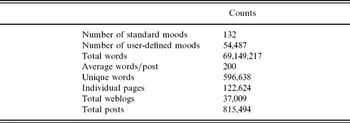
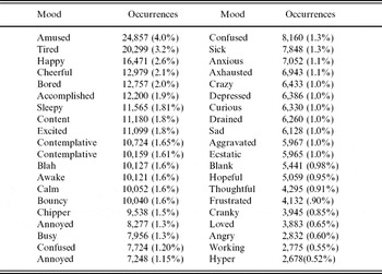
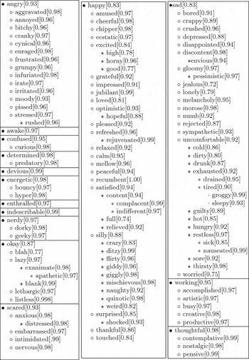
We used the blog data set that Mishne (Reference Mishne2005) collected for his research. The corpus contains 815,494 blog posts from Livejournal, a free weblog service used by millions of people to create weblogs. In Livejournal, users are able to optionally specify their current mood. To select their mood, users can choose from a list of 132 moods, or specify additional moods. We do not use the additional moods because very few posts are annotated with them. Some statistics of this corpus are shown in Table 1. From the total posts, only 77 per cent included an indication of the mood; we disregarded the rest. There are twenty-two posts per blog, on average. Table 2 shows the most frequent moods in the corpus, with their frequency counts. In the Livejournal weblog service, the moods are organized in a hierarchy, shown in Figure 1. Therefore, we will use this hierarchy to select the classes for each classification level, in the method that we propose in the next section.
Statistics about words and posts in the data set

The most frequent moods in corpus

The hierarchy of the 132 moods: ·, Level 1; ^, Level 2; ⋆, Level 3; *, Level 4; and ⋅, Level 5. The numbers in the brackets indicate the best F-measure that we obtained for each node, as discussed later in Section 5.3.

4 Our hierarchical approach to mood classification
Researchers have been developing new techniques to classify large volumes of documents and texts (e.g. directories or biomedical data), particularly when the number of classes is large and the classes have a hierarchical structure (Dekel, Keshet and Singer Reference Dekel, Keshet and Singer2004).
Hierarchical text categorization eliminates the assumption that categories are independent and instead tries to incorporate the interrelationship among the different categories. In a regular or flat text categorization approach, it is generally assumed that categories are independent and non-overlapping. This means that classification of an individual category is performed with the knowledge that all other categories are considered unrelated. In practice, however, categories tend to overlap and are not independent of each other (Wang, Zhou and Liew Reference Wang, Zhou and Liew1999).
Wang et al. (Reference Wang, Zhou and Liew1999) introduced two types of hierarchical text categorization methods: global and local. We explain these techniques below and show how we applied hierarchical categorization techniques in the mood classification task.
• Global Approach: In the global approach only one classifier discriminates all categories in a hierarchy. It differs from a flat categorization by considering the relations between the categories (using a similarity measure).
• Local Approach: In the local approach, a classifier is built for each internal node in the hierarchy. It proceeds in a down–top fashion, starting with selecting the categories of the first level and then recursively choosing among the lower-level categories (the children of the higher-level categories). There are two possibilities. The first is to train one classifier for all the categories in the first level of the hierarchy (multiclass problem). Then one classifier is trained for each of the classes in the first level, to differentiate among all its subclasses. The process continues if there are more levels. The second possibility is to build a single-class classifier for each node in each level of the hierarchy (a binary classifier that differentiates the class of the node from any other sibling classes).
We used the first approach, with SVM classifiers, because it is more efficient. We had to choose between using n-ary classification at each node, or n-binary classifiers at each node (where n is the number of classes at each hierarchical level). We decided that only the n-binary classifiers method is feasible in our case: since we have a large number of classes the other would take too much time. Not only would the training times be too long but the testing time would as well when running the classifiers on new data. Moreover, we used SVM classifiers, which are normally binary; thus we used binary classification. The results were combined by the Weka tool, in order to produce the final n-ary classifier.
We used the local approach, and we tried both ways mentioned above. For the first one, we used n-ary decision trees. For the second one, we used SVM classifiers, which are binary by nature, and then we combined them into n-ary classifiers using the Sequential Minimization Optimization (SMO) algorithm (Keerthi et al. Reference Keerthi, Shevade, Bhattacharyya and Murthy2001) from Weka. We briefly describe this method for combining classifiers in Section 4.1.
The second approach led to much better results. This is why we report only the SMO results in Section 5.2. In general, this approach has the disadvantage that it requires a large number of classifiers, because there are five hierarchy levels and there are many subclasses in each node of the hierarchy; but the SMO method in particular does not have this disadvantage because it has an efficient way to combine the classifiers (without storing them as intermediary classifiers). Using the approach with other classifiers (e.g. decision tress) would make it very difficult to manually manage the many intermediary classifiers, and the results are not likely to be good, since, for this task, decision trees did not lead to good results.
4.1 Combining SVM classifiers
In the past few years, many researchers have become interested in SVM classifiers because they have shown significant generalization performance on a wide range of problems (Vapnik Reference Vapnik1996; Burges Reference Burges1998). The SMO algorithm is a fast implementation of SVM introduced by Platt (Reference Platt, Schoelkopf, Burges and Smola1998): tests have shown that SMO is often much faster and has better scaling properties than other SVM implementations. However, it has a significant deficiency, caused by the manner in which it maintains and updates a single threshold value. Keerthi et al. (Reference Keerthi, Shevade, Bhattacharyya and Murthy2001) proposed a solution to this problem. They suggested using two threshold parameters and devised two modified versions of SMO that are more efficient than the original. Computational comparison on benchmark data sets showed that in most situations the modified versions perform significantly faster than the original SMO.
Another basic concern is that SVM is a binary classifier, and as such it cannot be used for problems with more than two classes. In the following, we examine the multiclass problem and the existing solutions.
The multiclass version of SMO uses the pairwise coupling procedure, which involves estimating class probabilities for each pair of classes, then coupling the estimates together. It starts by forming all the pairs of two classes, and training classifiers for them. Then all the pairwise decisions are combined to produce a multiclass classifier. The class that is finally chosen for a test instance is the class that has the highest number of pairs. The thresholds for the pairs of classes are optimized simultaneously, based on the training data. For more details, see (Hastie and Tibshirani Reference Hastie and Tibshirani1998).
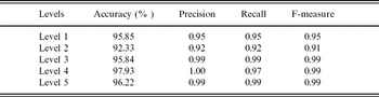
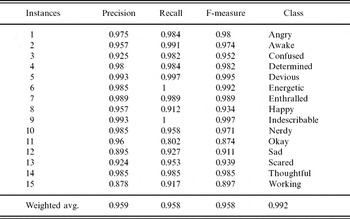
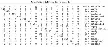
In Weka, the implementation of Platt's SMO algorithm for training a support vector classifier uses the polynomial or the radial basis function kernel. The implementation globally replaces all missing values and transforms nominal attributes into binary ones. It also normalizes all attributes by default. Moreover, Weka's SMO is extended to the multiclass problem using the pairwise classification (Hastie and Tibshirani Reference Hastie and Tibshirani1998) explained above. To obtain the best probability estimates, we used it with the option that fits logistic regression models to the outputs of the support vector machine. To show how Platt's SMO algorithm is used for classification in Weka, we show the Precision, Recall and F-measure for Level 1 of our hierarchal algorithm, later in the article, in Table 10. Also, Figure 3 illustrates the confusion matrix that Weka's SMO algorithm generates using binary classification for multiclass classification. Figure 3 shows the binary classification for the fifteen classes in Level 1. It compares each class with another class and shows the number of ‘correct’ and ‘incorrect’ instances for each class.
4.2 Feature set
A brief explanation of the features we used in our machine learning experiments follows. We used most of the features from Mishne (Reference Mishne2005), plus some additional sentiment orientation features, such as tagged words from the General Inquirer (Stone et al. Reference Stone, Dexter, Smith, Marshall and Ogilvie2007).
4.2.1 Frequency counts
Bag-of-Words (BoW) is the most common feature representation used in automatic text classification. Most text classification systems consider a document as simply a ‘bag of words’ and use the frequency of the words as features (Sebastiani Reference Sebastiani2002); we also represented the words by their frequencies. Part-of-Speech tags are another common feature of text classification systems. We used the frequency of words and Part-of-Speech tag counts as features and TreeTagger (Schmid Reference Schmid1994) to extract the Part-of-Speech tags.
4.2.2 Length-related features
Since blog posts vary in length, we also considered length features, such as the length of the document, the number of sentences and the average number of words. We split the sentences using a simple method and used standard punctuation marks as sentence delimiters.
4.2.3 Sentiment orientation
For emotion and mood classification, the sentiment orientation of some words can be a useful feature for predicting emotion and mood. For example, some emotions or moods, such as ‘annoyed’ and ‘frustrated’, are obviously negative while others, like ‘cheerful’ and ‘loved’, are clearly positive. So, it is expected that blogs posts with a positive aspect will, on average, have more positive orientation than negative blogs posts.
In our features set, we considered both the average word orientation and total orientation of a blog post as features. Determining the SO of a word is dependent on the method used for calculating it. We used several sources that are predictors for sentiment orientation. We calculated the total and the average orientation score for each document based on the words from the following resources:
• A list of 2,291 positive words and 1,915 negative words from the General Inquirer (Stone et al. Reference Stone, Dexter, Smith, Marshall and Ogilvie2007). These words were marked with tags such as active, passive, strong, weak, pleasure, pain, feeling (other than pain/pleasure), arousal, virtue, vice, overstated and understated.
• A list of 21,885 verbs and nouns that were automatically assigned a positive, negative, or neutral orientation score by Kim and Hovy (Reference Kim and Hovy2004).
They identified sentiments like the affective parts of opinions in their research. For this, they proposed a system that, for a given topic, automatically finds the people who hold opinions about that topic and the sentiment of each opinion. Their system contains a module for determining the sentiment of each word and a module for combining sentiments within a sentence. In their experiments, they used various models of classifying and combining sentiment at word and sentence levels, with promising results.
• A list of 1,718 adjectives with their scores of polarity values, constructed by using the method of Turney and Littman (Reference Turney and Littman2003). The method is based on measuring, for each word, its cooccurrence frequency on the web with a small set of positive adjectives and with a small set of negative adjectives.
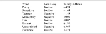
Examples of words and their sentiment orientation scores in Kim and Hovy's list and in the adjectives list are shown in Table 3.
Semtiment orientation values of words based on Kim and Hovy's list and on Turney and Littman's list

If there words had discrete values instead of numeric scores, we assigned a score of +1 to positive words and a score of −1 to negative words, and we calculated the sum and the average score of each text, for each of these three lists of words.
4.2.4 Special symbols
We used symbolic emotional icons (known as emoticons), which are printable characters intended to represent human emotions or attitudes. Emoticons are often horizontal textual representations of facial expressions (e.g. .:) = smile and ;= wink).
Today, emoticons are very popular in many domains, including blogs and chat rooms. The use of emoticons originated in email messages and quickly spread to other forms of online content. We used the nine most popular emoticons found in blog posts as features: tired, (:| ; smile, :); kiss, :-*; laughing, :d; sad, :(; love, :x; worried, :-s; surprise, :-o; angry, x-(.
5 Experiments and results
Our experiments and results are described in this section. We explain the performance of the simple flat classification into 132 moods and the performance of our hierarchy-based mood classification. We also explain the classification setting, then describe the experiments and results and investigate possible causes of errors.
5.1 Classification setting
We used the Weka data mining software (Witten and Frank Reference Witten and Frank2005) for our experiments. We chose SVM as the main classifier because it has been shown to perform very well in text classification tasks, including previous studies on mood classification. Moreover, SVMs are able to deal with a large number of features and instances (Joachims Reference Joachims1998). We experimented with a few other classifiers, such as Nave Bayes and Decision Trees, but the results for our tasks were lower than those of SVM. As explained in Section 4.1, we used the SMO algorithm from Weka to combine binary SVM classifiers into multiclass classifiers.
Our feature space is very large, so for efficiency, we reduced the feature space for the BoW features by using feature selection methods. We used the Chi-Square feature selection method, in order to keep only the first 5,000 features from the 43,109 initial BoW features. In addition, we used the six sentiment orientation scores (for each of the three resources, the average score of the words from the text that are also in the resource and their total score) and the emoticons.
5.2 Experiments
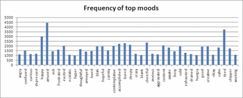
Our training data set for the experiments includes 144,129 instances, which vary among the 132 different moods. From all the posts, we randomly selected the 144,129 as training data, as well as 90,000 as test data. Figure 2 shows the top twenty-nine moods in our experimental data set (the training and test data that we selected). The distribution is slightly different than the distribution in the whole LiveJournal data described in Table 2.
Frequency of the top moods in the experimental data set.

Our first experiment consisted of a flat classification into the 132 moods, using the SMO classifier. The second experiment was performed to evaluate the hierarchical classification method. For this purpose, we first trained a classifier to classify into the fifteen categories from the first level of hierarchy (i.e. happy, sad, angry, okay, working, scared, awake, thoughtful, nerdy, indescribable, enthralled, determined, confuse, devious and energetic). In the next step, for each node from the first level of the hierarchy, we extracted the related instances and their mood labels. For example, for the node angry we selected all the documents that have the label angry, aggravated, annoyed, bitchy, cranky, cynical, enraged, frustrated, grumpy, infuriated, irate, irritated, moody, pissed and stressed. We then ran the classifier for each node in the second level. We repeated this procedure for each of the fifteen categories from the first level of the hierarchy and performed similar steps for the third, fourth and fifth level of the hierarchy.
For both sets of experiments above we ran our classifiers using BoW features and used BoW plus SO features (including emoticons). We found that adding the SO features greatly improves the classification results.
5.3 Results and discussion
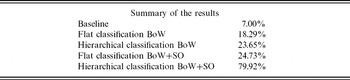
The results of the first experiment, the flat classification into 132 moods, achieved an accuracy of 24.73 per cent for BoW+SO features and 18.29 per cent for BoW features. This is an improvement compared with a baseline accuracy result of 7 per cent when always choosing the most frequent mood (baseline is the lower expectation in each level for a naive classifier that always chooses the most frequent class).
For the second experiment, the hierarchical approach, the accuracy for the classifier that classifies into one of the fifteen moods from the first level was 95.87 per cent for BoW+SO and almost 40 per cent for BoW, compared with a baseline of 15 per cent; the results for Level 1 are illustrated in Table 4.
Accuracy for the hierarchical classification in Level 1 for both BoW and BoW+SO features

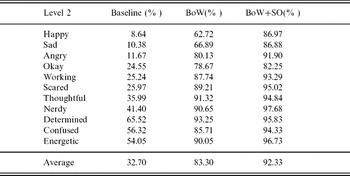
For the next step, we had fifteen potential classifiers in the second level, one for each node in the first level. We ultimately had eleven classifiers because four moods did not have any child branches in the hierarchy, so the classification for them was already completed. The average accuracy was 92.33 per cent for BoW+SO features, 83.30 per cent for BoW features only, and 32.70 per cent for a baseline of the most frequent class. The difference between the hierarchical approach with the features and the baseline is 59.63 per cent. There are several branches that have fewer children and show larger improvement and several others with many children that show lower performance improvement. For example, the moods happy, sad and angry have many child branches and the improvement is smaller, while the gain in performance is bigger for moods such as nerdy, which has two branches. Two branches means three classes: in this case generic nerdy and two more specific types of nerdy: geeky and dorky. The results for level two are shown in Table 5.
Accuracy for classification in Level 2 for both BoW and BoW+SO features

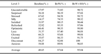
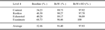
The results of the Level 3 classifier are shown in Table 6 and the results of Level 4 in Table 7. Level 5 has only one classifier, for tired, with an accuracy of 96.22 per cent for BoW+SO features and 87.61 per cent for BoW, with a baseline of 54.44 per cent.
Accuracy for classification in Level 3 for both BoW and BoW+SO features

Accuracy for the hierarchical classification in Level 4 for both BoW and BoW+SO features

Our experiments and results clearly show that the hierarchical classification leads to strong performance and is well suited for the task. The summary of results for each level, shown in Table 9, supports this claim.
In Table 8, we added average precision, recall and F-measure values for each level, for the best hierarchical classification setting (BoW+SO). The best F-measure for each leaf node is also indicated in square brackets in Figure 1, in order to show results for each of the 132 moods.
Overall average results in each level

To directly compare the results of the flat categorization to the results of the hierarchical classifiers, we cumulated the errors from all the levels. This provides a global accuracy of 79.92 per cent for all 132 classes for BoW+SO features and 18.29 per cent for the flat categorization. As illustrated in Table 9, the improvement in performance particularly especially when the sentiment orientation features are added. We believe the hierarchical method obtained better results because the classifiers are able to focus on a smaller number of classes and learn the distinctions between them.
The accuracy of the hierarchical classification when the classifiers from all the levels are applied successively (the errors from all the levels are multiplied), compared with the results of the flat classification, for both BoW and BoW+SO features

5.4 Error analysis
The error rates are higher for classes with many subclasses in the hierarchy, which is likely because the subclasses are very similar to each other, so the algorithm cannot find enough features to distinguish between them. Another possible cause of errors is the nature of the hierarchy. We used it as it was provided, but there are a few areas where it does not seem logical, for example, the class ‘silly’ being a subclass of ‘happy’. ‘Shocked’ and ‘surprised’ are also in the ‘happy’ class, when in reality they could be negative (as in pleasant surprise versus unpleasant surprise). In addition, some of the 132 possible classes are not well defined (e.g. recumbent and dorky), which could mean their labels have been arbitrarily chosen by the users who tagged their blogs.
To further investigate the difficulty of the task, we randomly selected a sample of blogs from those that were wrongly classified by our system. We wanted to see if human judges could classify them correctly (according to the tags chosen by the users who wrote the blogs) and, if not, determine the upper boundary of the accuracy that can be achieved by humans on this sample. An automatic system cannot be expected to produce better results than this upper boundary.
We cannot be certain that the data set was correctly annotated by the users who wrote the blogs. Some annotations might be wrong, which would lead to noise in the data set. We wanted to measure the agreement between human judges on this sample of data, to see how reliable the initial annotation is and how difficult the task is.
In general, the classification of opinions in texts is highly subjective, and this can cause disagreement between the annotations of human judges. Differences in the skills and focus of the judges, and ambiguity in both the annotation guidelines and the annotation task itself, also contribute to disagreement between judges (Passonneau Reference Passonneau2006). We attempted to determine the degree of agreement between judges with respect to annotating blogs by mood; it is important to note that we did this by using a sample of difficult blogs. If we had selected the sample from blogs correctly classified by the system, it is likely that human judges would be able to classify them correctly, and their annotations would be in agreement.
From our classification task for the first level of hierarchy, we randomly selected 58 instances which were wrongly predicted by our system. For these instances, the system was not able to predict the correct mood, as specified by the user of the LiveJournal. In order to provide more detailed results for Level 1 classification, we added precision, recall and F-measure for each subclass of this level (see Table 10) and a confusion matrix that shows the most frequent types of mistakes (see Figure 3). As explained in
Detailed results by class for Level 1

Confusion matrix for correctly classified instances and incorrectly classified instances in Level l.

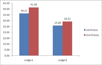
We performed additional analysis on this random sample that our classifier had classified wrongly. We asked two human judges to assess this random sample by annotating each text with one of the moods in the first level of hierarchy (i.e. indescribable, confused, angry, awake, devious, determined, energetic, enthralled, happy, nerdy, okay, sad, scared, thoughtful and working). They were also allowed to specify a second label and to write comments.
We first measured the correctness of each judge. As shown in Figure 4, the highest correctness score for classification by human judges was 36.79 per cent that means the upper boundary for our system's correctness on this sample of data cannot be higher than 36.79 per cent. These results prove that the classification task in our blog corpus is very difficult. If we include the second choices of the judges as correct labelling, the highest correctness score goes up to 41.38 per cent.
The correctness results by two judges A and B.

We then measured the degree to which the judges agreed when classifying a document into a correspondent mood. The agreement between judges A and B was 65.52 per cent, and the kappa value that compensates for agreement by chance (Cohen Reference Cohen1960) was 0.1889. The low agreement and kappa values prove that the task is difficult, even for human annotators. Also, some of the initial tags in the data set cannot be trusted. According to the comments of the human judges, the usual cause of a wrong tag is the existence of multiple moods in the same blog. The writer of the blog could choose only one mood, and it was most likely that he/she would select the mood they were in when they started writing, then their mood changed during the writing, and this was reflected in the text. The judges also mentioned that some blogs described different moods of several persons that the blog author was writing about.
6 Comparison to related work
Standard research on text classification is intended to detect the topic of documents. Less research has been done to detect specific features in the text (Sebastiani Reference Sebastiani2002), such as the gender of the writer (Koppel, Argamon and Shimoni Reference Koppel, Argamon and Shimoni2002) or authorship attribution (Koppel and Schler Reference Koppel and Schler2004).
In this article, we focused on mood classification. The task is difficult because of the distinctive aspects of mood in blogs. For example, a blogger can start writing in a certain mood, but the document can end with other content or mood. Some blogs are so intertwined that even human readers would have difficulty in identifying the mood and finding the relationship between the mood of the writer and the documents.
The work that is closest to our study is that of Mishne (Reference Mishne2005), who used binary SVM classifiers for mood classification of blog data. As mentioned, we used the data set that he collected from LiveJournal. Mishne used the only forty most frequent moods, as shown in Table 2. He trained a classifier for each of the forty moods, on different training sets, then showed the performance of each mood, based on various sizes of the corresponding training set. In order to compare our work with Mishne's results, we also classified into the forty most frequent moods. We obtained 84.89 per cent accuracy, while the baseline given by the most frequent class is very low at 6.62 per cent and a random choice among forty classes results in 2.5 per cent. Mishne reported an average accuracy of 67 per cent. He used a test set randomly chosen for each mood with a balanced distribution of classes, which means a 50 per cent baseline for an approach that considers one class versus all the other classes. Therefore, we are unable to directly compare our results to his because we cannot use precisely the same test set, even though our test set is randomly chosen from the same data.
However, to directly compare our method to Mishne's algorithm, we implemented Mishne algorithm, for forty classes (the most frequent moods) in order to reproduce his results. To do so, we used our data set and we only kept Mishne's features (based on our best knowledge for Mishne's features set), then we trained an SVM classifier on our training data. We obtained an accuracy of 58.13 per cent for this classifier on our test set, on which we obtained the accuracy of 84.89 per cent by our algorithm. This shows that our algorithm performs 27.26 percentage points better than Mishne's algorithm for the top forty moods.
In summary, the essential differences between our work and Mishne's is that we use all the 132 moods, not only the forty most-frequent ones, and we enhanced the feature set with more sentiment orientation features. In order to achieve good results for such a large number of classes, we chose to use a different approach (i.e. hierarchical classification).
Other research that investigated mood classification was done by Jung et al. (Reference Jung, Park and Myaeng2006) who proposed a hybrid approach to identify mood in blog texts. They used ConceptNet (Liu and Singh Reference Liu and Singh2004) and the Affective Norms English Words (Bradley and Lang Reference Bradley and Lang1999) list. To perform classification, they chose unique features from blogs and calculated statistical features such as term frequency, n-grams, and pointwise mutual information (PMI) for the SVM classification method. They also used a paragraph-level segmentation based on mood flow analysis and extracted their own blog data from LiveJournal. They show good classification results only when restricting the task to four mood types: happy, sad, angry and scared. In addition, they considered only documents with lengths of sentences between four and forty.
Liu et al. (Reference Liu, Lieberman and Selker2003) introduced another approach that works on a larger corpus and is based on ‘common-sense’ classification. They used a corpus of 400,000 facts about normal life in everyday life in the real world. They combined four linguistic models in order to recognize the affect. Their system analyzed the affective qualities of text, sentence by sentence. This has a practical value for people who want to evaluate the text they are writing.
Hierarchical categorization has been used for other text classification tasks. For example, Kiritchenko et al. (Reference Kiritchenko, Matwin, Nock and Famili2006) applied this approach to biomedical texts, using a hierarchy from gene ontology, with good results. Wilson et al. (Reference Wilson, Wiebe and Hoffmann2005) applied a hierarchical approach to classification of customer reviews as positive, negative or neutral. They used a very shallow hierarchy, to classify into neutral and polar texts and to further classify the polar texts into positive and negative, with mixed results.
7 Conclusions and future work
This article presented experiments of hierarchy-based mood classification of blog corpus. In addition, a hierarchical approach was considered to classify the data using the SVM algorithm. Our corpus was collected from Livejournal, an online service that allows users to post their personal thoughts. Our results showed that the hierarchical approach provides substantial performance improvement over flat classification. Classifying mood in blog text is a difficult task, due to the variety of users. However, our approach shows that if we classify blogs by using the mood hierarchy, we can achieve very good performance. We also showed that using SO features on top of BoW features greatly improves the classification results.
In future work, we plan to experiment with more features sets, types of features and feature selection methods.
Acknowledgments
The authors wish to thank Soo-Min Kim and Ed Hovy for providing their polarity-tagged lists.