





Let
 $N\geqslant 1$
be an integer and let
 $\mathit {SL}_N(\mathbb{Z} )$
be the modular group of integral matrices with determinant one. Our goal is to compute its cohomology groups with trivial coefficients, i.e.
 $H^q(\mathit {SL}_N(\mathbb{Z} );\mathbb{Z} )$
. These are known in the cases
 $N \leqslant 7$
:
 $N=2$
is classical (e.g. II.7, Ex.3 of [Reference Brück, Miller, Patzt, Sroka and Wilson9]),
 $N=3$
is due to Soulé [Reference Soulé47],
 $N=4$
is due to Lee and Szczarba [Reference Lee and Szczarba38], and
 $N=5,6,7$
are due to Elbaz-Vincent, Gangl and Soulé [Reference Elbaz-Vincent, Gangl and Soulé19].
In Theorem 5.2 below, we give partial information for the cases
 $N=8,9,10$
. For these calculations we follow mainly the methods of [Reference Lee and Szczarba38] and [Reference Elbaz-Vincent, Gangl and Soulé19], by investigating the Voronoi complexes associated to these modular groups.
Recall that a perfect form in N variables is a positive definite real quadratic form h on
 $\mathbb{R} ^N$
with given minimum m which is uniquely determined by its set of integral minimal vectors [Reference Martinet40](§3.2). Voronoi proved in [Reference Voronoi52] that there are finitely many perfect forms of rank N, modulo the action of
 $\mathit {SL}_N(\mathbb{Z} )$
. These are known for
 $N\leqslant 8$
(see §1 below). These finitely many orbits of perfect forms give the top-dimensional generators in the Voronoi complex; the rest of the complex is constructed from these perfect forms. Unfortunately, we cannot work with the full Voronoi complex for
 $N=8$
due to its size, which is beyond our computing capabilities, and we do not have complete information for
 $N>8$
. However, it turns out that it is possible to obtain partial information on the top and bottom parts of the Voronoi complexes for
 $8 \leqslant N \leqslant 10$
and conjecturally
 $N=11$
. In particular, we can enumerate the cells of lowest dimension explicitly using methods based on sublattices and relative index (cf. §2). For other cases, we can use linear programming in order to full enumeration in given cellular dimensions (cf. §3).
Voronoi used perfect forms to define a cell decomposition of the space
 $X_N^*$
of positive real quadratic forms, whose kernel is defined over
 $\mathbb{Q} $
. This cell decomposition (cf. §1.2) is invariant under
 $\mathit {SL}_N(\mathbb{Z} )$
, hence it can be used to give a chain complex which computes the equivariant homology of
 $X_N^*$
modulo its boundary: this is the Voronoi complex. On the other hand, this equivariant homology turns out to be isomorphic to the groups
 $H_q\big (\mathit {SL}_N(\mathbb{Z} ); \mathrm {St}_N\big )$
, where
 $\mathrm {St}_N$
is the Steinberg module (see [Reference Borel and J-P6] and §1.2.3 below). Finally, Borel–Serre duality asserts that the homology
 $H_*\big (\mathit {SL}_N(\mathbb{Z} ); \mathrm {St}_N\big )$
is dual to the cohomology
 $H^*\big (\mathit {SL}_N(\mathbb{Z} );\mathbb{Z} \big )$
(modulo torsion at primes
 $\leqslant N+1$
). Thus the results mentioned above give partial information about the cohomology of modular groups.
We will use this to obtain information about the algebraic K-theory of the integers. In particular, we will prove that the group
 $K_8(\mathbb{Z} )$
is trivial (Theorem 6.4) and discuss its consequences for the Kummer–Vandiver conjecture (cf. §7).
Organisation of paper: In §1, we recall the Voronoi theory of perfect forms and the Voronoi complex which computes the homology groups
 $H_q\big (\Gamma ;\mathrm {St}_\Gamma \big )$
with
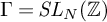 $\Gamma =\mathit {SL}_N(\mathbb{Z} )$
or
 $\mathit {GL}_N(\mathbb{Z} )$
. In §2, we give an explicit enumeration of the low-dimensional cells of the Voronoi complexes associated to
 $\Gamma $
. In §3, we present another method based on linear programming. In §4 we give a partial description of the Voronoi complex associated to modular groups of rank
 $N=8$
up to
 $12$
. In §5 we compute some homology groups of
 $\Gamma $
with coefficients in the Steinberg module and we explain how to compute part of the cohomology of
 $\mathit {SL}_N(\mathbb{Z} )$
and
 $GL_N(\mathbb{Z} )$
(modulo torsion) for
 $N\geqslant 8$
. In §6, we use these results to get some information on
 $K_m(\mathbb{Z} )$
for
 $m\geqslant 8$
and in particular show that
 $K_8(\mathbb{Z} )$
is trivial. In §7 we give some arithmetic applications.
Some of the enumerations of configurations of vectors had already been announced and used in [Reference Grushevsky, Hulek and Tommasi26]. Results concerning the triviality of
 $K_8(\mathbb{Z} )$
had already been announced in [Reference Elbaz-Vincent, Coulangeon, Gross and Nebe18, Reference Kupers33].
1 The Voronoi reduction theory
In this Section we recall some aspects of the Voronoi reduction theory [Reference Voronoi52, Reference Martinet40].
1.1 Perfect forms
Let
 $N \geqslant 2$
be an integer. We let
 $C_N$
be the set of positive definite real quadratic forms in N variables (i.e., real quadratic forms q such that
 $q(v)>0$
for any non-zero
 $v\in \mathbb{R} ^N$
). Given
 $h \in C_N$
, let
 $m(h)$
be the finite set of minimal vectors of h, i.e. vectors
 $v \in \mathbb{Z} ^N$
,
 $v \ne 0$
, such that
 $h(v)$
is minimal. A form h is called perfect when
 $m(h)$
determines h up to scalar: if
 $h' \in C_N$
is such that
 $m(h') = m(h)$
, then
 $h'$
is proportional to h.
Example 1.1. The form
 $h(x,y)=x^2+y^2$
has minimum 1 and precisely 4 minimal vectors
 $\pm (1,0)$
and
 $\pm (0,1)$
. This form is not perfect, because there is an infinite number of positive definite quadratic forms having these minimal vectors, namely the forms
 $h(x,y)=x^2+a x y+y^2$
where a is a non-negative real number less than 1. By contrast, the form
 $h(x,y)=x^2+x y+y^2$
also has minimum 1 and has exactly 6 minimal vectors, viz. the ones above and
 $\pm (1,-1)$
. Hence this form is perfect.
Denote by
 $C_N^*$
the set of non-negative real quadratic forms on
 ${\mathbb R}^N$
(i.e., real quadratic forms q such that
 $q(v)\geqslant 0$
for any
 $v\in \mathbb{R} ^N$
) the kernel of which is spanned by a proper linear subspace of
 ${\mathbb Q}^N$
, by
 $X_N^*$
the quotient of
 $C_N^*$
by positive real homotheties and by
 $\pi : C_N^* \to X_N^*$
the projection. Let
 $X_N = \pi (C_N)$
and
 $\partial X_N^* = X_N^* - X_N$
. Let
 $\Gamma $
be either
 $GL_N (\mathbb{Z} )$
or
 $\mathit {SL}_N (\mathbb{Z} )$
. The group
 $\Gamma $
acts on
 $C_N^*$
and
 $X_N^*$
on the right by the formula
 $$\begin{align*}h \cdot \gamma = \gamma^t \, h \, \gamma \, , \quad \gamma \in \Gamma \, , \ h \in C_N^* \, , \end{align*}$$
where h is viewed as a symmetric matrix and
 $\gamma ^t$
is the transpose of the matrix
 $\gamma $
. Voronoi proved that there are only finitely many perfect forms modulo the action of
 $\Gamma $
and multiplication by positive real numbers ([Reference Voronoi52], Thm. p.110). Table 1 gives the current state of the art on the enumeration of perfect forms.
Known results on the number of perfect forms up to dimension
 $9$
.

The classification of perfect forms of rank 8 was achieved by Dutour Sikirić, Schürmann and Vallentin [Reference Dutour Sikirić, Schürmann and Vallentin15, Reference Schürmann46], and for dimension
 $9$
has been done by Dutour Sikirić and van Woerden [Reference Dutour Sikirić and van Woerden16]. The corresponding classification for rank 7 was completed by Jaquet [Reference Jaquet-Chiffelle29], for rank 6 by Barnes [Reference Barnes3], for rank 5 and 4 by Korkine and Zolotarev [Reference Korkin and Zolotarev32, Reference Korkin and Zolotarev31], for dimension 3 by Gauss [Reference Gauss23] and for dimension 2 by Lagrange [Reference Lagrange36]. We refer to the book of Martinet [Reference Martinet40] for more details on the results up to rank 7. While the classification of perfect forms of higher rank is not well understood, we know from Bacher [Reference Bacher2] that the number of representatives grows at least exponentially with the rank and from van Woerden [Reference van Woerden51] is bounded by
 $e^{O(d^2\log (d))}$
for perfect forms of rank d.
1.2 The Voronoi complex
Notation 1.2. For any positive integer n we let
 ${\mathcal S}_n$
be the class of finite abelian groups the order of which has only prime factors less than or equal to n.
1.2.1 The cell complex
Given
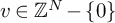 $v \in \mathbb{Z} ^N - \{ 0 \}$
, we let
 $\hat v \in C_N^*$
be the form defined by
 $$\begin{align*}\hat v (x) = (v \mid x)^2 \, , \ x \in {\mathbb R}^N \, , \end{align*}$$
where
 $(v \mid x)$
is the scalar product of v and x. The convex hull in
 $X_N^*$
of a finite subset
 $B \subset \mathbb{Z} ^N - \{ \mathbf 0 \}$
is the subset of
 $X_N^*$
which is the image under
 $\pi $
of the quadratic forms
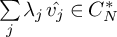 $\underset {j}{\sum } \, \lambda _j \, \hat {v_j}\in C_N^*$
, where
 $v_j \in B$
and
 $\lambda _j \geqslant 0$
. For any perfect form h, we let
 $\sigma (h) \subset X_N^*$
be the convex hull of the set
 $m(h)$
of its minimal vectors. Voronoi proved in [Reference Voronoi52], §§8-15, that the cells
 $\sigma (h)$
and their intersections, as h runs over all perfect forms, define a cell decomposition of
 $X_N^*$
, which is invariant under the action of
 $\Gamma $
. We endow
 $X_N^*$
with the corresponding
 $CW$
-topology. If
 $\tau $
is a closed cell in
 $X_N^*$
and h is a perfect form with
 $\tau \subset \sigma (h)$
, we let
 $m(\tau )$
be the set of vectors v in
 $m(h)$
such that
 $\hat v$
lies in
 $\tau $
. Any closed cell
 $\tau $
is the convex hull of
 $m(\tau )$
, and for any two closed cells
 $\tau $
,
 $\tau '$
in
 $X_N^*$
we have
 $m(\tau ) \cap m(\tau ') = m (\tau \cap \tau ')$
.
We shall now recall an explicit description of the Voronoi complex and its differential from [Reference Elbaz-Vincent, Gangl and Soulé19].
Let
 $d(N) = N(N+1)/2-1$
be the dimension of
 $X_N^*$
and
 $n \leqslant d(N)$
a natural integer. We denote by
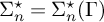 $\Sigma _n^\star = \Sigma _n^\star (\Gamma )$
a set of representatives, modulo the action of
 $\Gamma $
, of those cells of dimension n in
 $X_N^*$
which meet
 $X_N$
, and by
 $\Sigma _n =\Sigma _n(\Gamma ) \subset \Sigma _n^\star (\Gamma )$
the cells
 $\sigma $
for which any element of the stabiliser
 $\Gamma _{\sigma }$
of
 $\sigma $
in
 $\Gamma $
preserves orientation.
Let
 $V_n$
be the free abelian group generated by
 $\Sigma _n$
. We define as follows a map
 $$\begin{align*}d_n \colon V_n \to V_{n-1} \,. \end{align*}$$
For each closed cell
 $\sigma $
in
 $X_N^*$
we fix an orientation of
 $\sigma $
, i.e. an orientation of the real vector space
 ${\mathbb{R} } (\sigma )$
of symmetric matrices spanned by the forms
 $\hat v$
with
 $v \in m(\sigma )$
. Let
 $\sigma \in \Sigma _n$
and let
 $\tau '$
be a face of
 $\sigma $
which is equivalent under
 $\Gamma $
to an element in
 $\Sigma _{n-1}$
(i.e.
 $\tau '$
neither lies on the boundary nor has elements in its stabiliser reversing the orientation). Given a positive basis
 $B'$
of
 ${\mathbb R} (\tau ')$
we get a basis B of
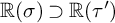 ${\mathbb R} (\sigma )\supset {\mathbb R} (\tau ')$
by appending to
 $B'$
a vector
 $\hat v$
, where
 $v \in m(\sigma ) - m(\tau ')$
. We let
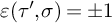 $\varepsilon (\tau ' , \sigma ) = \pm 1$
be the sign of the orientation of B in the oriented vector space
 ${\mathbb R} (\sigma )$
(this sign does not depend on the choice of v).
Next, let
 $\tau \in \Sigma _{n-1}$
be the (unique) cell equivalent to
 $\tau '$
and let
 $\gamma \in \Gamma $
be such that
 ${\tau '= \tau \cdot \gamma }$
. We define
 $\eta (\tau , \tau ') = 1$
(resp.
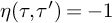 $\eta (\tau , \tau ') = -1$
) when
 $\gamma $
is compatible (resp. incompatible) with the chosen orientations of
 ${\mathbb R} (\tau )$
and
 ${\mathbb R} (\tau ')$
.
Finally, if
 $\sigma \in \Sigma _n$
and
 $\tau \in \Sigma _{n-1}$
, we define the incidence number
 $[\sigma :\tau ]$
for the Voronoi complex as
 $$ \begin{align} [\sigma:\tau]=\sum_{\tau'} \eta (\tau , \tau') \, \varepsilon (\tau' , \sigma)\, , \end{align} $$
where
 $\tau '$
runs through the set of faces of
 $\sigma $
which are equivalent to
 $\tau $
. If
 $\tau $
is not equivalent to a face of
 $\sigma $
, we set
 $[\sigma :\tau ]=0$
. The following map is thus well defined
 $$ \begin{align} d_n (\sigma) = \sum_{\tau \in \Sigma_{n-1}} [\sigma:\tau] \, \tau \,. \end{align} $$
It turns out that the map d generalises the usual differential of regular CW-complex to the case of the Voronoi complex (which is not regular CW-complex).
1.2.2 The associated equivariant spectral sequence
According to Section VII.7 of [Reference Brown8], there is a spectral sequence
 $E_{pq}^r$
converging to the equivariant homology groups
 $H_{p+q}^{\Gamma } (X_N^* , \partial X_N^*; \mathbb{Z} )$
of the pair
 $(X_N^* , \partial X_N^*)$
, with
 $E^1$
-page given by
 $$\begin{align*}E_{pq}^1 = \bigoplus_{\sigma \in \Sigma_p^\star} H_q (\Gamma_{\sigma}; \mathbb{Z}_{\sigma}) \, , \end{align*}$$
where
 $\mathbb{Z} _{\sigma }$
is the orientation module of the cell
 $\sigma $
and, as above,
 $\Sigma _p^\star $
is a set of representatives, modulo
 $\Gamma $
, of the p-cells
 $\sigma $
in
 $X_N^*$
which meet
 $X_N$
. Notice that the action of
 $\Gamma _{\sigma }$
on
 $\mathbb{Z} _{\sigma }$
is given by
 $\eta $
described above. Since
 $\sigma $
meets
 $X_N$
, its stabiliser
 $\Gamma _{\sigma }$
is finite and, by Lemma 4.1 in §3 below, the order of
 $\Gamma _{\sigma }$
is divisible only by primes
 $p \leqslant N+1$
. Therefore, when q is positive, the group
 $H_q (\Gamma _{\sigma }; \mathbb{Z} _{\sigma })$
lies in
 ${\mathcal S}_{N+1}$
.
When
 $\Gamma _{\sigma }$
happens to contain an element which changes the orientation of
 $\sigma $
, the group
 $H_0 (\Gamma _{\sigma }; \mathbb{Z} _{\sigma })$
is killed by
 $2$
, otherwise
 $H_0 (\Gamma _{\sigma }; \mathbb{Z} _{\sigma })\cong \mathbb{Z} $
. Therefore, modulo
 ${\mathcal S}_2$
, we have
 $$\begin{align*}E_{n\,0}^1 = \bigoplus_{\sigma \in \Sigma_n} \mathbb{Z}_{\sigma} \, , \end{align*}$$
and the choice of an orientation for each cell
 $\sigma $
gives an isomorphism between
 $E_{n\,0}^1$
and
 $V_n$
.
Proposition 1.3 [Reference Elbaz-Vincent, Gangl and Soulé19, §3.3, p.591-592]
The differential
 $$\begin{align*}d_n^1 \colon E_{n\,0}^1 \to E_{n-1,0}^1 \end{align*}$$
coincides, up to sign, with the map
 $d_n$
defined in 1.2.1.
As pointed out on p.589 of [Reference Elbaz-Vincent, Gangl and Soulé19], the identity
 $d_{n-1} \circ d_n = 0$
gives us a non-trivial test of our explicit computations.
Notation 1.4. The resulting complex
 $(V_\bullet ,d_\bullet )$
is denoted by
 ${\mathrm {Vor}}_\Gamma $
and is called the Voronoi complex.
1.2.3 The Steinberg module
Let
 $T_N$
be the spherical Tits building of
 $\mathit {SL}_N$
over
 ${\mathbb Q}$
, i.e. the simplicial set obtained as the nerve of the ordered set of non-zero proper linear subspaces of
 ${\mathbb Q}^N$
. The Solomon–Tits theorem says that
 $T_N$
is homotopy equivalent to wedge of
 $(N-2)$
-spheres, see Theorem IV.5.2 of [Reference Brück, Miller, Patzt, Sroka and Wilson9]. Thus the reduced homology
 $\tilde H_q (T_N;\mathbb{Z} )$
of
 $T_N$
with integral coefficients is zero except when
 $q = N-2$
, in which case

is by definition the Steinberg module. According to Proposition 1 of [Reference Soulé50], the relative homology groups
 $H_q (X_N^* , \partial X_N^*; \mathbb{Z} )$
are zero except when
 $q = N-1$
, and
 $$\begin{align*}H_{N-1} (X_N^* , \partial X_N^*; \mathbb{Z}) = {\mathrm{St}}_N \,. \end{align*}$$
From this it follows that, for all
 $m \in {\mathbb{N} }$
,
 $$ \begin{align} H_m^{\Gamma} (X_N^* , \partial X_N^*; \mathbb{Z}) \cong H_{m-N+1} (\Gamma; {\mathrm{St}}_N) \end{align} $$
(see e.g. §3.1 of [Reference Soulé50]). Combining this equality with the previous sections, we obtain:
Proposition 1.5. For arbitrary positive integers
 $N>1$
and m. We have the following isomorphism modulo
 ${\mathcal {S}}_{N+1}$
 $$ \begin{align} H_{m-N+1} (\Gamma; {\mathrm{St}}_N) \cong H_m ({\mathrm{Vor}}_\Gamma) \quad \mod {\mathcal{S}}_{N+1}. \end{align} $$
2 Small cells of quadratic forms
The method described in [Reference Martinet39], Sections 9.2 and 9.3, though not very efficient, can be used to classify cells of dimension
 $\frac {n(n+1)}2-t$
for small values of t with explicit calculations; these are the ‘small cells’ referred to in the title and will allow us to give an explicit enumeration of the lowest dimensional cells of the Voronoi complexes associated to
 $\Gamma $
which will be used in §4.
2.1 Minimal classes and the perfection rank
Our aim is the study of the Voronoi complex in a given (cellular) dimension n. We shall make use of Watson’s index theory, a theory which is better understood in terms of lattices. For this reason we first recall some data of the ‘dictionary’ which links lattices with quadratic forms. We refer to [Reference Martinet40] for further details.
We identify a quadratic form q with the
 $n\times n$
symmetric matrix A such that
 ${q(x)=X^{t} A X}$
, where X is the column-vector of the components of
 $x\in \mathbb{R} ^n$
. Let E be an n-dimensional Euclidean space, on which the norm of x is
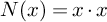 $N(x)=x\cdot x$
. With a lattice
 $\Lambda \subset E$
(discrete subgroup of E of rank n) and a basis
 ${\mathcal B}=(e_1,\dots ,e_n)$
for
 $\Lambda $
over
 $\mathbb{Z} $
, we associate the Gram matrix
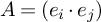 $A=(e_i\cdot e_j)$
of
 ${\mathcal B}$
and the corresponding positive definite quadratic form q. The minimum of
 $\Lambda $
and its set
 $m(\Lambda )$
of minimal vectors correspond to the same notions for quadratic forms. We denote by
 $s(\Lambda )$
the number of pairs of minimal vectors of
 $\Lambda $
(or of q). Besides this ‘kissing number’ an important invariant is the perfection rank r, the definition of which we recall now. Let
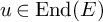 $u\in \operatorname {\mathrm {End}}(E)$
. The transpose of u is the endomorphism
 $^tu$
such that
 $u(x)\cdot y=x \cdot ^tu(y)$
for all
 $x,y\in E$
. We say that u is symmetric if
 $^tu=u$
. Let
 $\operatorname {\mathrm {End}}^s(E)$
be the space of all symmetric endomorphisms. Given a line
 $D\subset E$
, we denote by
 $p_D\in \operatorname {\mathrm {End}}^s(E)$
the orthogonal projection to D, and write
 $p_x$
if
 $D=\mathbb{R} \,x$
for some
 $x\ne 0$
in E. Note the formulae
 $p_x(y)=\frac {x\cdot y}{x\cdot x}\,x\ {\text { and }}\ \operatorname {\mathrm {Mat}}({\mathcal B}^*,{\mathcal B},p_x)=X X^{t}$
where
 ${\mathcal B}^*$
is the dual basis to
 ${\mathcal B}$
, defined by
 $e_i\cdot e_j^*=\delta _{i,j}$
. We denote by
 $\mathrm {Sym}_n(\mathbb{R} )$
the real vector space of
 $n\times n$
symmetric matrices with coefficients in
 $\mathbb{R} $
.
Definition 2.1. The perfection rank of a family
 $D_1,\dots ,D_\ell $
(
 $\ell $
a positive integer) of lines in E is the dimension of the span in
 $\operatorname {\mathrm {End}}^s(E)$
of the projections
 $p_{D_i}$
. A perfection relation on the set
 $\{D_i\}$
is a non-trivial
 $\mathbb{R} $
-linear relation of the form
 $\sum \lambda _i\,p_{D_i}=0$
. The perfection rank r of a lattice
 $\Lambda $
is the perfection rank of the set of lines
 $\mathbb{R} \,x$
,
 $x\in m(\Lambda )$
; that of a quadratic form q is the rank in
 $\mathrm {Sym}_n(\mathbb{R} )$
of the set
 $\{X X^{t}\}$
,
 $X\in m(q)$
.
We partition the space
 ${\mathcal L}$
of lattices into minimal classes by the relation
 $\Lambda \sim \Lambda '$
if and only if there exists
 $u\in \mathit {GL}(E)$
such that
 $u(\Lambda )=\Lambda '$
and
 $u(m(\Lambda ))=m(\Lambda ')$
, and order the minimal classes by the relation
 ${\mathcal C}\prec {\mathcal C}'$
if and only if there exists
 $\Lambda \in {\mathcal C}$
and
 $\Lambda '\in {\mathcal C}'$
such that
 $m(\Lambda )\subset m(\Lambda ')$
.
The dictionary above establishes a one-to-one correspondence between the set of minimal classes on the one hand, and the set of cells up to equivalence of (positive, definite) quadratic forms having a given minimum on the other hand. These are finite sets.
In the sequel, we restrict ourselves to well-rounded lattices (or forms), those for which the minimal vectors span E. The following proposition provides an easy test to decide whether two lattices belong to the same minimal class. Given a lattice
 $\Lambda $
and a basis
 ${\mathcal B}$
for
 $\Lambda $
, and a set
 $S'$
of representatives of pairs of minimal vectors of
 $m(\Lambda )$
, let T be the
 $n\times s(\Lambda )$
matrix of the components of the vectors of
 $S'$
on
 ${\mathcal B}$
, and let
 $B=T\,T^{t}$
. This is the barycenter matrix of
 $(\Lambda ,{\mathcal B})$
. Its equivalence class under
 $\mathit {GL}_n(\mathbb{Z} )$
does not depend on
 ${\mathcal B}$
.
Proposition 2.2. Two lattices belong to the same minimal class if and only if their barycenter matrices define the same class under
 $\mathit {GL}_n(\mathbb{Z} )$
.
Proof. This is Proposition 9.7.2 of [Reference Martinet40].
Lemma 2.3. Any perfection relation in
 $\operatorname {\mathrm {End}}^s(E)$
between projections to vectors of E may be written in the form
 $\sum _{x\in S}\,\lambda _x p_x=\sum _{y\in T}\,\mu _y p_y$
where
 $\lambda _x,\,\mu _y$
are strictly positive and S and T span the same subspace of E.
Proof. Getting rid of the zero coefficients, we obtain a relation of this kind for convenient subsets
 $S,T$
of E, and we may moreover assume that the vectors
 $x,y$
have norm
 $1$
. Applying this relation on a vector
 $z\in T^\perp $
and taking the scalar products with z, we obtain the equality
 $\sum _{x\in S}\,\lambda _x\,(x\cdot z)^2=0$
which shows that z also belongs to
 $S^\perp $
. We have thus proved the inclusion
 $T^\perp \subset S^\perp $
, i.e.,
 ${\langle } S{\rangle } \subset {\langle } T{\rangle }$
, and exchanging S and T shows that
 ${\langle } S{\rangle }={\langle } T{\rangle }$
.
Remark 2.4. By the lemma above, a perfection relation with non-zero coefficients between vectors which span an m-dimensional subset F of E involves at least
 $2m$
vectors. This is optimal for all
 $m\geqslant 2$
, as shown by the union of two orthogonal bases
 ${\mathcal B}$
and
 ${\mathcal B}'$
for F, since the sum of the orthogonal projections to the vectors of
 ${\mathcal B}$
and
 ${\mathcal B}'$
both add to the orthogonal projection to F. This construction of perfection relations accounts for those of the lattice
 $\mathbb {D}_4$
, since the set of minimal vectors
 $S(\mathbb {D}_4)$
is the union of three orthogonal frames.
Theorem 2.5. The perfection rank r of a well-rounded n-dimensional lattice with kissing number
 $s\leqslant n+5$
is equal to s.
Proof. By definition of the perfection rank we have
 $r\leqslant s$
, and if
 $r<s$
, there exists a perfection relation with support
 $2m$
vectors of some m-dimensional subspace F of E. We have
 $s\geqslant n+m$
, hence
 $m\leqslant 5$
. Now for a lattice L of dimension
 $n\leqslant 5$
, one has
 $s=n$
except if
 $L\sim \mathbb {D}_4$
or if
 $n=5$
and L has a
 $\mathbb {D}_4$
-section having the same minimum. Since
 $s(\mathbb {D}_4)=12$
, we then have
 $s\geqslant n+8$
, a contradiction.
Notice that in the above theorem the bound
 $s-n\leqslant 5$
is optimal; see Example 2.7 below.
2.2 Watson’s index theory and very small cells
2.2.1 Codes associated with well-rounded lattices
Let
 $\Lambda $
be a well-rounded lattice, let
 $e_1,\dots ,e_n$
be n independent minimal vectors of
 $\Lambda $
, and let
 $\Lambda '$
be the sublattice of
 $\Lambda $
generated by the
 $e_i$
. Let
 $\gamma _n$
be the Hermite constant in dimension n [Reference Martinet40](§2.2). Then the index
 $[\Lambda :\Lambda ']$
is bounded from above by
 $\gamma _n^{n/2}$
and so is the annihilator d of
 $\Lambda /\Lambda '$
. The maximal index
 $\imath (\Lambda )$
of a well-rounded lattice
 $\Lambda $
is the largest possible value of
 $[\Lambda :\Lambda ']$
for a pair
 $(\Lambda ,\Lambda ')$
as above.
Every element of
 $\Lambda $
can be written in the form
 $x=\dfrac {a_1 e_1+\dots +a_n e_n}d,\ a_i\in \mathbb{Z} $
,
and if
 $d>1$
the systems
 $(a_1,\dots ,a_n)\ \mod d$
can be viewed as the words of a
 $\mathbb{Z} /d\mathbb{Z} $
-code. The codes arising this way have been classified for n up to
 $8$
in [Reference Martinet39] (which relies on previous work by Watson, Ryshkov and Zahareva) and for
 $n=9$
in [Reference Keller, Martinet and Schürmann30]. The paper [Reference Martinet39] relied on calculations which were feasible essentially by hand (together with some checks made using PARI [25]). This is no longer possible beyond dimension
 $8$
, and indeed [Reference Keller, Martinet and Schürmann30] needed the use of a linear programming package, which was implemented on MAGMA [Reference Bosma, Cannon and Playoust7].
By averaging on the automorphism group of the code (see Proposition 8.5 of [Reference Martinet39]), one proves that if some code
 ${\mathcal C}$
of length n can be lifted to a pair
 $(\Lambda ,\Lambda ')$
(we then say that
 ${\mathcal C}$
is admissible), then there exist
 $\Lambda $
and
 $\Lambda '$
which are invariant under
 $\mathrm {Aut}({\mathcal C})$
. Then the minimum
 $s_{\min }$
of s (over well-rounded lattices) is attained on such a lattice
 $\Lambda $
, and the minimal class of
 $\Lambda $
depends uniquely on
 ${\mathcal C}$
.
By inspection of the tables of [Reference Martinet39] (Tableau 11.1) and [Reference Keller, Martinet and Schürmann30] (Tables 2-10), one proves:
Proposition 2.6. Let
 $d\geqslant 2$
and
 $n\leqslant 9$
, and let
 ${\mathcal C}$
be an admissible
 $\mathbb{Z} /d\mathbb{Z} $
-code. Then either
 ${\mathcal C}$
can be lifted to a pair
 $(\Lambda ,\Lambda ')$
with
 $m(\Lambda )=\{\pm e_i\}$
, or we have
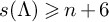 $s(\Lambda )\geqslant n+6$
for every lift of
 ${\mathcal C}$
.
Before going further we give some more precise results on the index theory. The most useful tool is Watson’s identity, relying vectors
 $e_1,\dots ,e_n$
of a basis for E, a vector
 $e=\frac {a_1 e_1+\dots +a_n e_n}d$
, and the vectors
 $e^{\prime }_i:=e-\operatorname {\mathrm {sgn}}(a_i)e_i\,$
:
 $$\begin{align*}\left(\Big(\sum_{i=1}^n|a_i|\Big)-2d\right)N(e)= \sum_{i=1}^n|a_i|\big(N(e^{\prime}_i)-N(e_i)\big)\,.\end{align*}$$
Applied to minimal vectors
 $e_i$
of a lattice
 $\Lambda ={\langle } e_i,e{\rangle }$
, this proves the lower bound
 $\sum \,\lvert a_i\rvert \geqslant 2d$
, and moreover shows that the vectors
 $e^{\prime }_i$
for which
 $a_i\ne 0$
are minimal whenever
 $\sum \,\lvert a_i\rvert =2d$
.
Example 2.7. Let
 $n=6$
,
 $d=3$
and let
 $(e_1,\dots ,e_6)$
be a basis for E with
 $N(e_i)=1$
and constant scalar products
 $e_i\cdot e_j=t$
. Let
 $\Lambda ={\langle } e_1,\dots ,e_6,e{\rangle }$
where
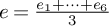 $e=\frac {e_1+\dots +e_6}3$
. Then for
 $\frac 1{10}<t<\frac 14$
(e.g.,
 $t=\frac 15$
), the minimum of
 $\Lambda $
is 1,
 $m(\Lambda )=\{\pm e_i,\pm e^{\prime }_i\}$
, and the perfection relations are proportional to
 $\sum p_{e_i}=\sum p_{e^{\prime }_i}$
, so that
 $s(\Lambda )=12=n+6$
and
 $r=11=s-1$
. This is a consequence of the fact that we can associate canonically a perfection relation with every Watson identity [Reference A-M and Martinet4](Proposition 2.5).
2.2.2 Primitive minimal classes (or cells)
Let
 ${\mathcal C}$
be a minimal class. For every lattice
 $\Lambda \in {\mathcal C}$
,
 $\widetilde \Lambda =\Lambda \perp m\mathbb{Z} $
, where
 $m=$
minimum of
 $\Lambda $
, is a lattice in
 $E\times \mathbb{R} $
, which defines a minimal class
 ${\mathcal C}'={\mathcal C}+\mathbb{Z} $
of dimension
 $n+1$
, containing all direct sums
 $\Lambda \oplus m\mathbb{Z} $
close enough to
 $\widetilde \Lambda $
. We say that
 ${\mathcal C}$
is primitive if it does not extend by this process a class of dimension
 $n-1$
.
Among n-dimensional (well-rounded) minimal classes, that of
 $\mathbb{Z} ^n$
, which has
 $\imath =1$
and
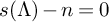 $s(\Lambda )-n=0$
, plays a special role. Indeed, let
 ${\mathcal C}$
be a minimal class and let
 $e_1,\dots ,e_n$
be independent minimal vectors of some lattice
 $\Lambda \in {\mathcal C}$
, and let
 $\Lambda '\subset \Lambda $
be the lattice with basis
 $(e_1,\dots ,e_n)$
. Let
 $I_1\subset \{1,\dots ,n\}$
be the support of the code defined by
 $(\Lambda ,\Lambda ')$
(
 $I_1=\emptyset $
if
 $\Lambda =\Lambda '$
) and let
 $I_2$
be the set of subscripts which occur as components of minimal vectors distinct from the
 $\pm e_i$
(
 $I_2=\emptyset $
if
 $s(\Lambda )=n$
). Set
 $I=I_1\cup I_2$
and
 $m=\lvert I\rvert $
. If
 ${\mathcal C}$
is not the minimal class of
 $\mathbb{Z} ^n$
, then I is not empty and
 ${\mathcal C}$
extends a minimal class of dimension
 $m\geqslant 2$
.
Therefore, to list minimal classes up to equivalence it suffices to list those which are primitive and then complete the list with those of the form
 ${\mathcal C}'\oplus \mathbb{Z} $
for some class
 ${\mathcal C}'$
of dimension
 $n-1$
.
2.2.3 Classes with
 $s(\Lambda )=n$

Theorem 2.8. The numbers of minimal classes of well-rounded lattices
 $\Lambda $
with
 $s(\Lambda )=n$
and
 $n\leqslant 9$
having a given index
 $\imath $
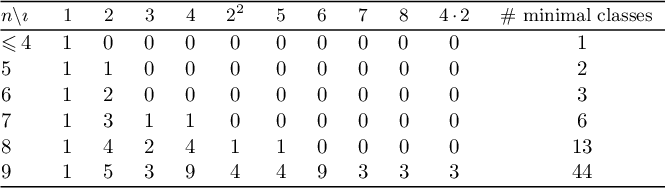
are displayed in Table 2.
Number of minimal classes of well-rounded lattices
 $\Lambda $
with
 $s(\Lambda )=n$
and
 $n\leqslant 9$
according to the quotient.

Proof. The lattices
 $\Lambda $
with
 $s(\Lambda )=n$
contain a unique sublattice
 $\Lambda '$
generated by minimal vectors of
 $\Lambda $
, and
 $\Lambda '$
has a unique basis up to permutation and changes of signs. Hence the classification of minimal classes coincide with the index classification. We mainly need to consider the results from [Reference Martinet39] and [Reference Keller, Martinet and Schürmann30]. According to the previous section, for index 2 (resp. 3) there is one primitive class if
 $n \geqslant 5$
(resp.
 $n \geqslant 7$
), hence
 $n-4$
(resp.
 $n-6$
) cells. Similarly for cyclic quotients of order 4 and
 $n \geqslant 9$
there are
 $n-4$
primitive cells, but only three if
 $n = 8$
, one if
 $n = 7$
and none if
 $n \leqslant 6$
, which for
 $n = 7, 8, 9$
yields 1, 4 and 9 cells of cyclic type with
 $\imath = 4$
. In the case
 $\imath =4$
but with
 $\Lambda /\Lambda '$
of type
 $2^2$
(i.e.
 $\imath =2^2$
), the condition is that the corresponding binary code must be of weight
 $w \geqslant 5$
. This implies
 $\ell \geqslant 8$
, and if
 $\ell = 8$
(resp.
 $\ell = 9$
), we are left with one code, with weight distribution
 $(5^2 , 6)$
(resp. three codes, with weight distributions
 $(5^2 , 8)$
,
 $(5, 6, 7)$
and
 $(6^3 )$
). As a result we got four primitive cells. Finally we just have to read in the tables of [Reference Martinet39](Tableau 11.1) and [Reference Keller, Martinet and Schürmann30](Tables 2-10) for index
 $\imath \geqslant 5$
and
 $n\leqslant 9$
for all admissible codes for which
 $s(\Lambda )=n$
is possible.
To deal with slightly larger values of
 $s(\Lambda )$
, we first establish an as short as possible list of a priori possible index systems, then test for minimal equivalence the putative classes obtained from this list, and finally construct explicitly lattices in the putative class or prove that such a class does not exist. This third step is the most difficult and it is hopeless to deal with relatively large values of
 $s(\Lambda )$
or of n without using efficient linear programming methods, as seen in §3.
2.3 Lattices
$\Lambda $
with
$s(\Lambda )=1$
or
$s(\Lambda )=2$


Consider a lattice
 $\Lambda _0$
having a basis of minimal vectors
 ${\mathcal B}=(e_1,\dots ,e_n)$
and
 $t=s(\Lambda _0)-n$
other minimal vectors
 $x_i=\sum _{i=1}^n\,a_{i,j} e_j$
,
 $1\leqslant j\leqslant t$
. The
 $m\times m$
determinants (
 $m\leqslant \min (t,n)$
) extracted from the matrix
 $(a_{i,j})$
are the characteristic determinants of Korkine and Zolotarev (cf. Chapter 6 from [Reference Martinet40]). With every characteristic determinant
 $d\ne 0$
they associate a lattice
 $\Lambda ^{\prime }_0$
of index
 $\lvert d\rvert $
in
 $\Lambda _0$
. This shows that if
 $\imath (\Lambda _0)=1$
, then
 $d=0$
or
 $\pm 1$
; in particular all
 $a_{i,j}$
are
 $0$
or
 $\pm 1$
.
3 Enumeration of configurations of vectors
In this section we explain the algorithms used for enumerating the configurations of vectors in dimension
 $n\in \{8, \dots , 12\}$
and rank
 $r=n$
,
 $n+1$
or above.
Our approach computes first the configurations of vectors in rank
 $r=n$
and then from this enumeration gets the configurations in rank
 $r=n+1$
, then
 $n+2$
and so on. The number of cases explodes with the dimension n and rank r as one expects and the computation is thus quite slow. However, for the case
 $r=n$
an additional problem occurs: the known bounds on the determinant of vector configurations are suboptimal. All computations rely on the ability to test if a configuration of shortest vectors of a positive definite matrix can be derived from a given configuration of vectors.
3.1 Testing realisability of vector family
In [Reference Keller, Martinet and Schürmann30] an algorithm for testing realisability of vector families by solving linear programs was introduced. We describe below the needed improvements of our strategy in order to reach higher dimensions. We refer to [Reference Schrijver45] for an account of the classical theory of linear programming.
Given m affine functions
 $(\phi _i)_{1\leqslant i\leqslant m}$
on
 $\mathbb {R}^n$
and another (linear) function
 $\phi $
the linear program is to minimise
 $\phi (x)$
for x subject to the constraints
 $\phi _i(x)\geqslant 0$
. Define
 ${{\mathcal P} = \{x\in \mathbb {R}^n, \text {~s.t.}\;\phi _i(x)\geqslant 0\}}$
. The linear program is called feasible if
 ${\mathcal P}\not = \emptyset $
and the elements of
 ${\mathcal P}$
are called feasible solutions. If
 $\phi $
is bounded from below on
 ${\mathcal P}$
then the inferior limit is denoted
 $opt({\mathcal P}, \phi )$
and is attained by one feasible solution. Any feasible solution will satisfy
 $\phi (x) \geqslant opt({\mathcal P}, \phi )$
The dual problem is to maximise the value of m such that there exist
 $\beta _i$
with
 $$ \begin{align*} \phi = m + \sum_{i=1}^m \beta_i \phi_i \text{~with~} \beta_i\geqslant 0 \end{align*} $$
Any feasible solution of the dual problem will give us
 $\phi (x) \geqslant m$
and the maximum value of such m will be exactly
 $opt({\mathcal P}, \phi )$
by a theorem of von Neumann [Reference Schrijver45](§7.4). In other words, any feasible solution
 $(m, \beta _i)$
of the dual problem will give us
 $opt({\mathcal P}, \phi )$
.
Let A be an
 $n \times n$
matrix with real coefficients and set
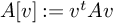 $A[v]:=v^t A v$
for any
 $v \in \mathbb{R} ^n$
. Given a configuration of vectors
 ${\mathcal V}$
the basic linear program to be considered is
 $$ \begin{align*} \begin{array}{rl} \text{minimize} & \lambda\\ \text{with} & \lambda=A[v] \text{~for~} v\in {\mathcal V}\\ & A[v] \geqslant 1 \text{~for~} v\in \mathbb{Z}^n - \{0\} - {\mathcal V} \end{array} \end{align*} $$
If the optimal value satisfies
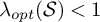
 $\lambda _{opt} < 1$
, then
 ${\mathcal V}$
is realisable, otherwise not.
The main issue is that the above linear program has an infinity of defining inequalities and so instead we consider the program restricted to a finite subset, i.e. the linear inequalities:
 $$ \begin{align*} A[v] \geqslant 1 \text{~for~} v\in {\mathcal S} \text{~with~} {\mathcal S} \text{ finite~and~ } {\mathcal S}\subset \mathbb{Z}^n - \{0\} - {\mathcal V}. \end{align*} $$
It can happen that the equalities
 $\lambda =A[v]$
for
 $v\in {\mathcal V}$
have no solution with
 $\lambda \neq 0$
. In that case
 ${\mathcal V}$
is not realisable.
It can also happen that the linear program is unbounded, that is, solutions with arbitrarily negative value of
 $\lambda $
are feasible. In that case we append
 $2 {\mathcal V}$
to
 ${\mathcal S}$
.
Thus if those restrictions are implemented then the linear program has an optimal rational solution
 $A_{opt}({\mathcal S})$
of optimal value
 $\lambda _{opt}({\mathcal S})$
.
According to the solution of the linear program we can derive following conclusions:
-
1. If
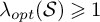
$\lambda _{opt}({\mathcal S}) \geqslant 1$
then we can conclude that the vector configuration is not realisable. -
2. If
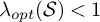
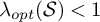
$\lambda _{opt}({\mathcal S}) < 1$
and
$A_{opt}({\mathcal S})$
is positive definite then we compute
$\operatorname {\mathrm {Min}}(A_{opt}({\mathcal S}))$
.-
(a) If
$\operatorname {\mathrm {Min}}(A_{opt}({\mathcal S})) = {\mathcal V}$
then the configuration is realisable -
(b) Otherwise we cannot conclude. But we can insert the vectors in the difference
$\operatorname {\mathrm {Min}}(A_{opt}({\mathcal S})) - {\mathcal V}$
into
${\mathcal S}$
and iterate.
-
-
3. If
$\lambda _{opt}({\mathcal S}) < 1$
and
$A_{opt}({\mathcal S})$
is not of full rank then we can compute some integer vector in the kernel of
$A_{opt}({\mathcal S})$
and insert them into
${\mathcal S}$
and iterate. -
4. If
$\lambda _{opt}({\mathcal S}) < 1$
and
$A_{opt}({\mathcal S})$
is of full rank but not positive semidefinite then we can compute an integer vector v such that
$A_{opt}({\mathcal S}) [v] < \lambda _{opt}({\mathcal S})$
and insert it into
${\mathcal S}$
and iterate.










Thus we can iterate until we obtain either feasibility of the vector configuration or unfeasibility. In practice a naive implementation of this algorithm can be very slow and we need to apply a number of improvements in order to get reasonable running time:
-
1. The dimension of the program is
$n(n+1)/2 - r$
and this is quite large. We can use symmetries in order to get smaller program. Namely we compute the group of integral linear transformations preserving
${\mathcal V}$
and impose that the matrix A also satisfies this invariance. -
2. Even after symmetry reduction the linear programs have many inequalities and are hard to solve. In our implementation we use cdd [Reference Fukuda22] based on exact arithmetic and provides solutions of the linear program and its dual in exact rational arithmetic. However, cdd uses the simplex algorithm and is very slow in some cases. Thus the idea is to use floating point arithmetic and the glpk program [24] which has better algorithms and can solve linear programs in double precision. From the approximate solution we can guess in most cases a feasible rational solution of the linear program and its dual. If both give the same value, then we have resolved our linear program. If this approach fails, then we fall back to the more expensive in time cdd. In all cases, we only accept a solution if it has a corresponding dual solution.
-
3. If the matrix
$A_{opt}({\mathcal S})$
is of full rank but not positive definite then there exists an eigenvector
$w\in \mathbb{R} ^n$
of eigenvalue
$\alpha < 0$
. We then use the sequence of vectors with
$$ \begin{align*} w^i = \left( Near(i w_1), Near(i w_2), \dots, Near(i w_n) \right). \end{align*} $$
$Near(x)$
being the nearest integer to a real number x. As i increases
$w^i$
approaches the direction of the vector w. Thus there is an index
$i_0$
such that
$w^{i_0}\not = 0$
and
$A_{opt}({\mathcal S}) [w^{i_0}] < \lambda _{opt}({\mathcal S})$
and this vector
$w^{i_0}$
can be inserted into
${\mathcal S}$
. The problem is that in many cases the matrix
$A_{opt}({\mathcal S})$
is very near to being positive definite and the negative eigenvalue will be very small. Thus we first try double precision with the Eigen template matrix library [Reference Guennebaud and Jacob27] for the computation of the eigenvector and vector
$w^{i_0}$
. If this fails then we use the arbitrary precision floating point library mpfr [Reference Fousse, Hanrot, Lefèvre, Pélissier and Zimmermann21], still with Eigen and progressively increase the number of digits until a solution is found.
-
4. An issue is for the initial vector set. In our implementation we set
but there could be better choice for initial vector set.
$$ \begin{align*} {\mathcal S} = {\mathcal V} \cup \left\lbrace x \pm e_i \pm e_j\text{~for~}x\in {\mathcal V} \text{~and~}1\leqslant i,j\leqslant n\right\rbrace - \{0\} \end{align*} $$
-
5. We apply LLL reduction [Reference Cohen13] to the vector configuration. Namely, we define a positive definite matrix
and apply the LLL reduction to it in order to get a reduction matrix
$$ \begin{align*} A_{{\mathcal V}} = \sum_{v\in {\mathcal V}} v^t v \end{align*} $$
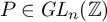
$P\in \mathit {GL}_{n}(\mathbb {Z})$
. The matrix
$P\in \mathit {GL}_n(\mathbb{Z} )$
is then used to reduce
${\mathcal V}$
as well. The use of LLL reduction reduces the maximal size of the coefficients and dramatically reduces the number of iterations needed to get a result. Hence we use it systematically.








When all those methods are implemented we manage to do the realisability tests in reasonable time.
A variant of the realisability algorithm mentioned above is to consider a family of vector
 ${\mathcal V}$
of rank r and return a realisable configuration of vectors
 ${\mathcal W}$
of rank r if it exists that contains
 ${\mathcal V}$
. It suffices in the case
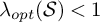 $\lambda _{opt}({\mathcal S}) < 1$
and
 $A_{opt}({\mathcal S})$
to distinguish between vectors of
 $\operatorname {\mathrm {Min}}(A_{opt})$
that increases the rank and vectors that do not increase the rank.
3.2 Enumeration of configurations of vectors with
$r=n$

In [Reference Keller, Martinet and Schürmann30] it is proved that for a configuration
 $\{\pm v_1, \dots , \pm v_n\}$
of shortest vectors of a lattice, we have
 $$ \begin{align*} \vert \det(v_1, \dots, v_n)\vert \leqslant \sqrt{\gamma_n^n} \,. \end{align*} $$
As it turns out this upper bound on the determinant is tight for dimension
 $n\leqslant 8$
but not in dimensions
 $9$
and
 $10$
. An additional problem is that
 $\gamma _n$
is known exactly only for
 $n\leqslant 8$
and
 $n=24$
. Our strategy is thus to simply enumerate the vector configurations up to the best upper bound that we have on the determinant.
For dimension
 $10$
, combined with the known upper bound on
 $\gamma _{10}$
this gives an upper bound of
 $59$
on the indexes of the relevant lattices [Reference Keller, Martinet and Schürmann30]. If one uses the conjectured value of
 $\gamma _{10}$
then one gets
 $36$
as upper bound in dimension
 $10$
. It will turn out that the maximal possible determinant is
 $16$
.
A key aspect of the enumeration is to enumerate first the cases where the quotient
 $\mathbb {Z}^n / L$
has the structure of a prime cyclic group. This is important since if a prime p is unfeasible then any vector configuration with determinant divisible by p is unfeasible as well. It is also important since our enumeration goes prime by prime for composite determinants. For
 $d=p_1\times \dots \times p_r$
we first do the enumeration of vector configurations of determinant
 $p_1$
, then
 $p_1p_2$
and so on.
In the case of lattices of index p with p prime we consider a lattice L spanned by
 $e_1=(1, 0,\dots , 0)$
, …,
 $e_n = (0, \dots , 0, 1)$
and
 $$ \begin{align*} e_{n+1} = \frac{1}{p} (a_1, \dots, a_n), a_i\in \mathbb{Z} \end{align*} $$
such that
 $(e_1, \dots , e_n)$
is the configuration of shortest vectors of a lattice. By standard reductions, we can assume that
-
•
$a_1\leqslant a_2 \leqslant \dots \leqslant a_n$
-
• and
$1\leqslant a_i\leqslant \left \lfloor p/2\right \rfloor $
.


Since p is prime
 $e_{n+1}$
can be replaced by
 $k e_{n+1}$
for any
 $1\leqslant k\leqslant p-1$
. Thus we can assume the vector
 $e_{n+1}$
to be lexicographically minimal among all possible vectors.
It turns out that lexicographically minimal vector configurations can be enumerated by exhaustive enumeration without having to store in memory the list of candidates. The idea is as follows: if
 $(a_1, \dots , a_n)$
is lexicographically minimal, then
 $(a_1, \dots , a_{n-1})$
is also lexicographically minimal. Lexicographic minimality only requires
 $(p-1)n$
multiplications and reductions to be tested. Thus we enumerate all configuration up to length
 $n-1$
and then extend this enumeration to length n by adding all possible feasible candidates. For
 $n=10$
and
 $p=59$
we have
 $16301164$
possible vector configurations and for each of them we test realisability.
When the enumeration for index p is done we can continue the enumeration up to index
 $p p'$
by taking all feasible lattices of index p and considering all their sublattices of index
 $p'$
up to action of the symmetry group. Thus we get a set of a priori feasible lattices for which we can apply our realisability algorithm and get a list of lattices of index
 $p p'$
. For
 $n=10$
the most complex case of this kind is
 $49 = 7^2$
.
By doing prime by prime up to
 $59$
in this way we are able to get all configurations of shortest vectors in dimension
 $10$
, we find
 $283$
different lattices. For dimension
 $n=11$
, we were only able to go up to index
 $45$
and we got in total
 $6674$
possible sublattices. The list is not proved to be complete but it is reasonable to conjecture that this list is complete since the maximum determinant of a realisable vector configuration is
 $32$
. For dimension
 $n=12$
, we managed only to go up to index
 $30$
and found
 $454576$
different vector configurations and it seems that this list is far from complete.
3.3 Enumeration of configurations of vectors with
$r>n$

For the case
 $r=n+1$
and
 $r=n+2$
we have proved in [Reference Dutour Sikirić, Hulek and Schürmann14] that the relevant cones are simplicial. In [Reference Dutour Sikirić, Hulek and Schürmann14] an algorithm is given for getting the full list of configuration vectors in those ranks. The only improvement to this algorithm is that the integer points are obtained by an exhaustive enumeration procedure since zsolve proved too slow.
For rank
 $r=n+3$
and above simpliciality is not a priori true, though it is expected to hold in rank
 $n+3$
and
 $n+4$
. Thus we need a different approach to the enumeration. If we have a configuration of vectors
 ${\mathcal V}'$
in dimension n and rank
 $r>n+2$
then it necessarily contains a n-dimensional configurations
 ${\mathcal V}$
of rank
 $r-2$
and two n-dimensional configurations
 ${\mathcal W}_1$
and
 ${\mathcal W}_2$
of rank
 $r-1$
such that
 $$ \begin{align*} {\mathcal V} \subset {\mathcal W}_i \subset {\mathcal V}'. \end{align*} $$
Our approach is as follows:
-
1. We first enumerate the configurations of vectors in dimension n and rank
$r-2$
and
$r-1$
. -
2. We determine all the orbits of pairs
$({\mathcal V}, {\mathcal W})$
with
${\mathcal V}$
of dimension n rank
$r-2$
,
${\mathcal W}$
of dimension n rank
$r-1$
. -
3. For any configuration
${\mathcal V}$
of dimension n rank
$r-2$
there is a finite number of configurations of vectors of dimension n rank
$r-1$
containing it. We can thus enumerate all the pairs
$({\mathcal W}_1, {\mathcal W}_2)$
containing
${\mathcal V}$
and check if
${\mathcal W}_1\cup {\mathcal W}_2$
is contained in a realisable family of vectors.


3.4 Obtained enumeration results
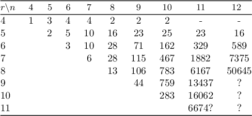
By combining all above enumeration methods, we can obtain the number of orbits of perfect domains for small r and n.
Proposition 3.1. The number of orbits of cones in the perfect cone decomposition for rank
 $r\leqslant 12$
and dimension n at most
 $11$
(the result for
 $r=n=11$
is conjectural) are given in Table 3.
Known number of orbits of cones in the perfect cone decomposition for rank
 $r\leqslant 12$
and dimension n at most
 $11$
(the result for
 $r=n=11$
is conjectural).

Remark 3.2. For dimension
 $n=11$
,
 $12$
we do not have a full enumeration, however the partial configurations obtained are already instructive. In all dimensions
 $n\leqslant 10$
the orientations of the well-rounded families of vectors with
 $s=n$
(i.e., the orientation of the associated cells of dimension n in
 $X^*_n$
) were found not to be preserved by their stabiliser. However, this changes with five well-rounded configurations known in dimension
 $11$
and
 $12$
in dimension
 $12$
. One such configuration in dimension
 $11$
is
 $e_{5}+e_{6}+e_{7}+e_{10}-e_{3}$
,
 $e_{11}-e_{2}-e_{10}$
,
 $e_{3}+e_{9}$
,
 $e_{4}+e_{6}+e_{8}-e_{2}-e_{9}$
,
 $e_{1}+e_{2}+e_{3}$
,
 $e_{4}+e_{7}+e_{11}-e_{6}$
,
 $e_{8}+e_{9}-e_{7}$
,
 $e_{1}+e_{5}-e_{11}$
,
 $e_{4}+e_{5}$
,
 $e_{1}-e_{8}$
,
 $e_{10}$
and it has a stabiliser of order
 $4$
which is the minimum known so far. It seems reasonable to expect that there are well-rounded vector configurations with stabiliser of order
 $2$
, i.e. only antipodal operation. We know just one well-rounded configuration in dimension
 $12$
whose orbit under
 $\mathit {GL}_{12}(\mathbb {Z})$
splits into two orbits under
 $\mathit {SL}_{12}(\mathbb {Z})$
. One representative is
 $e_{6}-e_{1}-e_{2}-e_{3}-e_{4}$
,
 $e_{6}-e_{7}-e_{8}$
,
 $e_{9}-e_{3}-e_{6}-e_{10}-e_{11}-e_{12}$
,
 $e_{7}+e_{12}-e_{1}-e_{2}-e_{5}-e_{8}$
,
 $e_{11}-e_{1}-e_{4}-e_{5}-e_{6}-e_{10}$
,
 $e_{2}$
,
 $e_{4}+e_{8}-e_{7}$
,
 $e_{9}$
,
 $e_{10}$
,
 $e_{3}+e_{5}+e_{7}+e_{9}-e_{1}$
,
 $e_{11}$
,
 $e_{12}$
.
Remark 3.3. The above data for
 $r\leqslant 7$
recover the computations of [Reference Elbaz-Vincent, Gangl and Soulé19] (cf. Figures 1 and 2) and [Reference Lee and Szczarba38].
4 Homology of the Voronoi complexes
4.1 Preliminaries
Recall the following simple fact, cf. p.602 of [Reference Elbaz-Vincent, Gangl and Soulé19], which is relevant for understanding the action of
 $\mathit {GL}_N(\mathbb{Z} )$
on
 $X_N$
:
Lemma 4.1.
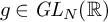
-
• Assume that p is a prime and
$g \in {\mathit {GL}}_N ({\mathbb R})$
has order p. Then
$p \leqslant N+1$
. -
• The action of
${\mathit {GL}}_N ({\mathbb R})$
on the symmetric space
$X_N$
preserves its orientation if and only if N is odd.


Remark 4.2. We can give a more precise statement regarding the torsion in
 $\mathit {GL}_N(\mathbb{Z} )$
. Let p be an odd prime and k a positive integer. Set
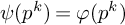 $\psi (p^k) = \varphi (p^k)$
,
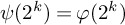 $\psi (2^k) = \varphi (2^k)$
if
 $k>1$
and set
 $\psi (2)=\psi (1)=0$
. For an arbitrary
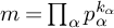 $m = \prod _{\alpha } p_{\alpha }^{k_{\alpha }}$
define
 $\psi (m) = \sum _{\alpha } \psi (p_{\alpha }^{k_{\alpha }})$
. According to the crystallographic restriction theorem, an elementary proof of which is given as Theorem 2.7 of [Reference Kuzmanovich and Pavlichenkov35], an element of order m occurs in
 $\mathit {GL}_{N}(\mathbb {Z})$
if and only if
 $\psi (m)\leqslant N$
.
4.2 The Voronoi complexes in low dimensions
From the computations of §2 and §3, we deduce the following cardinalities.
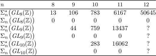
Proposition 4.3. The number of low-dimensional cells in the quotient
 $(X^*_N,\partial X^*_N)/\mathit {GL}_N(\mathbb{Z} )$
is given by Table 4.
Cardinality of
 $\Sigma _n$
and
 $\Sigma _n^\star $
for
 $N=8,9,10$
(empty slots denote zero).

The explicit data can be retrieved at the url https://github.com/elbazvip/Voronoi-complexes-database. For convenience to the reader, we give below a set of representatives in the case
 $s(\Lambda )=n=8$
.
Proposition 4.4. A set of representatives for the 13 well-rounded cells of
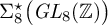 $\Sigma _8^\star \big (\mathit {GL}_8(\mathbb{Z} )\big )$
is given by the following matrices:
 $$ \begin{align*} \begin{pmatrix} 0 &0 &0 &0 &0 &-1 &0 &0 \\ 0 &-1 &0 &0 &0 &1 &0 &0 \\ 0 &-1 &0 &1 &0 &1 &1 &0 \\ 0 &0 &0 &1 &0 &1 &0 &0 \\ 0 &-1 &-1 &1 &0 &0 &0 &0 \\ 1 &1 &1 &0 &0 &0 &0 &0 \\ 0 &2 &0 &-2 &0 &-1 &-1 &-1 \\ 0 &-1 &-1 &1 &1 &1 &1 &1 \end{pmatrix},\begin{pmatrix} 0 &0 &1 &1 &1 &0 &0 &0 \\ 0 &0 &-1 &-2 &-1 &0 &0 &0 \\ 0 &0 &-2 &-2 &-2 &0 &-1 &0 \\ 0 &0 &-1 &-1 &-1 &0 &0 &-1 \\ 0 &-1 &-1 &-1 &-2 &0 &0 &0 \\ 1 &1 &1 &1 &1 &0 &0 &0 \\ -1 &1 &3 &3 &3 &0 &1 &1 \\ 0 &-1 &-2 &-2 &-2 &1 &0 &0 \end{pmatrix},\\\begin{pmatrix} 0 &1 &1 &0 &0 &0 &-1 &0 \\ 0 &-1 &-2 &0 &0 &0 &1 &0 \\ 0 &-1 &-2 &0 &0 &0 &1 &1 \\ 0 &-1 &-1 &0 &0 &-1 &0 &0 \\ 0 &-1 &-1 &0 &0 &1 &0 &0 \\ 1 &1 &1 &0 &0 &0 &0 &0 \\ 0 &1 &3 &0 &-1 &0 &0 &0 \\ -1 &-1 &-2 &1 &1 &0 &0 &0 \end{pmatrix},\begin{pmatrix} 0 &0 &1 &-1 &0 &0 &0 &-1 \\ 0 &0 &-2 &1 &0 &0 &0 &1 \\ 0 &-1 &-2 &1 &0 &1 &0 &1 \\ 0 &-1 &-1 &0 &0 &0 &0 &1 \\ 0 &-1 &-1 &1 &0 &0 &0 &0 \\ 1 &1 &1 &0 &0 &0 &0 &0 \\ 0 &2 &3 &-2 &0 &-1 &-1 &-2 \\ 0 &-1 &-2 &1 &1 &1 &1 &1 \end{pmatrix},\\\begin{pmatrix} -1 &-2 &0 &0 &1 &1 &1 &-1 \\ 0 &1 &0 &0 &0 &-1 &-1 &0 \\ 0 &1 &0 &0 &-1 &-1 &-1 &2 \\ 0 &0 &1 &0 &0 &0 &0 &-1 \\ 0 &-1 &0 &0 &0 &0 &1 &-1 \\ 0 &1 &0 &0 &-1 &-1 &-2 &1 \\ 0 &-1 &-1 &-1 &1 &1 &1 &0 \\ 1 &1 &1 &1 &0 &0 &0 &0 \end{pmatrix},\begin{pmatrix} 0 &0 &0 &-1 &0 &0 &0 &1 \\ 0 &-1 &0 &1 &0 &0 &1 &0 \\ 0 &1 &0 &0 &-1 &0 &-1 &0 \\ 1 &-1 &0 &1 &1 &0 &0 &0 \\ 0 &1 &-1 &0 &0 &0 &0 &0 \\ -1 &1 &1 &0 &0 &0 &0 &0 \\ 0 &2 &0 &-1 &-1 &-1 &-1 &0 \\ 1 &-2 &0 &1 &1 &1 &1 &0 \end{pmatrix},\\\begin{pmatrix} 0 &0 &0 &0 &-1 &1 &0 &0 \\ 0 &0 &1 &-1 &-1 &0 &0 &1 \\ 0 &0 &0 &1 &1 &-1 &0 &-1 \\ 0 &0 &0 &0 &0 &0 &1 &1 \\ 0 &0 &-1 &0 &0 &-1 &0 &0 \\ 1 &0 &1 &0 &0 &0 &0 &0 \\ 0 &0 &1 &-1 &-1 &1 &0 &0 \\ 0 &1 &-1 &1 &1 &0 &0 &0 \end{pmatrix},\begin{pmatrix} -1 &1 &-1 &-2 &-1 &-1 &-2 &0 \\ 0 &0 &1 &1 &0 &0 &1 &0 \\ -1 &0 &-1 &-1 &-1 &0 &-1 &1 \\ 0 &-1 &0 &1 &1 &1 &2 &0 \\ 1 &0 &2 &1 &1 &0 &1 &0 \\ 0 &1 &0 &0 &0 &-1 &-1 &0 \\ 0 &1 &-1 &-1 &-1 &-1 &-1 &0 \\ 1 &0 &1 &1 &1 &1 &1 &0 \end{pmatrix},\\\begin{pmatrix} 1 &1 &-1 &-1 &-1 &0 &0 &1 \\ -1 &0 &1 &1 &1 &-1 &-1 &0 \\ 0 &0 &-1 &0 &0 &1 &1 &0 \\ -1 &0 &1 &0 &0 &-1 &0 &0 \\ 0 &-1 &1 &1 &0 &0 &0 &0 \\ 0 &0 &0 &0 &1 &1 &0 &0 \\ 1 &0 &-1 &-1 &0 &0 &0 &0 \\ 1 &1 &0 &0 &0 &0 &0 &0 \end{pmatrix},\begin{pmatrix} 1 &1 &0 &0 &-1 &0 &0 &0 \\ -1 &0 &0 &-1 &1 &0 &-1 &0 \\ 1 &-1 &0 &1 &0 &0 &0 &0 \\ -1 &0 &0 &-1 &0 &0 &-1 &1 \\ -1 &-1 &0 &0 &0 &1 &1 &0 \\ 0 &-1 &-1 &0 &1 &0 &0 &0 \\ 1 &1 &0 &1 &0 &0 &0 &0 \\ 1 &1 &1 &0 &0 &0 &0 &0 \end{pmatrix},\\[6pt]\begin{pmatrix} 0 &0 &0 &0 &0 &1 &0 &-1 \\ 0 &0 &0 &1 &0 &1 &0 &1 \\ 0 &0 &0 &-1 &0 &-1 &1 &0 \\ -1 &0 &1 &-1 &0 &-2 &0 &0 \\ 0 &1 &-1 &0 &1 &1 &0 &0 \\ 0 &-1 &1 &1 &0 &0 &0 &0 \\ 0 &0 &1 &-1 &0 &-1 &0 &0 \\ 1 &1 &-1 &1 &0 &1 &0 &0 \end{pmatrix},\begin{pmatrix} 0 &-1 &0 &0 &1 &0 &-1 &0 \\ 0 &1 &-1 &0 &0 &0 &0 &1 \\ 0 &-1 &1 &0 &0 &0 &1 &0 \\ 1 &1 &-1 &0 &-1 &1 &0 &0 \\ -1 &-1 &1 &1 &0 &0 &0 &0 \\ -1 &0 &0 &0 &1 &0 &0 &0 \\ 1 &2 &-2 &0 &0 &0 &0 &0 \\ 0 &-1 &2 &0 &0 &0 &0 &0 \end{pmatrix},\\[6pt]\begin{pmatrix} 0 &0 &0 &1 &0 &0 &0 &-1 \\ -1 &0 &0 &-1 &0 &0 &1 &0 \\ 0 &0 &-1 &-1 &0 &0 &1 &0 \\ 0 &0 &-1 &0 &0 &0 &1 &1 \\ 0 &-1 &0 &-1 &0 &0 &0 &0 \\ 1 &1 &1 &1 &0 &0 &0 &0 \\ 0 &0 &1 &1 &0 &-1 &-2 &0 \\ 0 &0 &-1 &-1 &1 &1 &1 &0 \end{pmatrix}.\qquad\qquad\qquad\qquad\end{align*} $$
We can check the inequivalence of the above matrices using the command qfisom from PARI [25]. As all cells have their orientations changed, we deduce the following central result for the homology of the Voronoi complex.
Theorem 4.5. The groups
 $H_k({\mathrm {Vor}}_{\mathit {GL}_N(\mathbb{Z} )})$
are zero modulo
 $\mathcal {S}_2$
for
 $N=8$
and
 $k \leqslant 12$
,
 $N=9,10$
and
 $k<12$
.
Remark 4.6. In the case
 $N=12$
we cannot prove so far that the list of 12-dimensional cells of
 ${\mathrm {Vor}}_{\mathit {GL}_N(\mathbb{Z} )}$
is complete (even if heuristically it seems the case).
5 Cohomology of modular groups
5.1 Borel–Serre duality
According to Borel and Serre, Theorems 11.4.4 and 11.5.1 of [Reference Borel and J-P6], the group
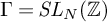 $\Gamma =\mathit {SL}_N(\mathbb{Z} )$
or
 $\mathit {GL}_N(\mathbb{Z} )$
is a virtual duality group with dualising module
 $$\begin{align*}H^{v(N)} (\Gamma; \mathbb{Z} [\Gamma]) = {\mathrm{St}}_N \otimes \tilde{\mathbb{Z}} \, , \end{align*}$$
where
 $v(N) = N(N-1)/2$
is the virtual cohomological dimension of
 $\Gamma $
and
 $\tilde {\mathbb{Z}} $
is the orientation module of
 $X_N$
. It follows that there is a long exact sequence

where
 $\hat H^*$
is the Farrell cohomology of
 $\Gamma $
[Reference Farrell20].
From Lemma 4.1 and the Brown spectral sequence, X (4.1) of [Reference Brück, Miller, Patzt, Sroka and Wilson9], we deduce that
 $\hat H^* (\Gamma , \tilde{\mathbb{Z}} )$
lies in
 ${\mathcal S}_{N+1}$
. Therefore
 $$ \begin{align} H_n (\Gamma; \mathrm{\mathrm{St}}_N) \equiv H^{v(N)-n} (\Gamma; \tilde{\mathbb{Z}}) \, , \ \text{modulo } {\mathcal S}_{N+1}. \end{align} $$
When N is odd, then
 $\mathrm {GL}_N (\mathbb{Z} )$
is the product of
 $\mathrm {SL}_N (\mathbb{Z} )$
by
 $\mathbb{Z} / 2$
, therefore
 $$\begin{align*}H^m (\mathrm{GL}_N (\mathbb{Z}); \mathbb{Z}) \equiv H^m (\mathrm{SL}_N (\mathbb{Z}); \mathbb{Z}) \, , \ \text{modulo } {\mathcal S}_2. \end{align*}$$
When N is even, then the action of
 $\mathrm {GL}_N (\mathbb{Z} )$
on
 $\tilde{\mathbb{Z}} $
is given by the sign of the determinant (see Lemma 4.1) and Shapiro’s lemma gives
 $$ \begin{align} H^m (\mathrm{SL}_N (\mathbb{Z}) , \mathbb{Z}) = H^m (\mathrm{GL}_N (\mathbb{Z}) , M) \, , \end{align} $$
with
 $$\begin{align*}M = \mathrm{Ind}_{\mathrm{SL}_N (\mathbb{Z})}^{\mathrm{GL}_N (\mathbb{Z})} \, \mathbb{Z} \equiv \mathbb{Z} \oplus \tilde{\mathbb{Z}} \, , \ \text{modulo } {\mathcal S}_2. \end{align*}$$
5.2 Homology of modular groups with coefficients in the Steinberg module
Corollary 5.1. The groups
 $H_{k-N+1} (\mathit {GL}_N(\mathbb{Z} ); {\mathrm {St}}_N)$
are trivial modulo
 $\mathcal {S}_{N+1}$
for
 ${N=8,9,10}$
and
 $k=8,\ldots ,11$
(assuming
 $k\geqslant N$
).
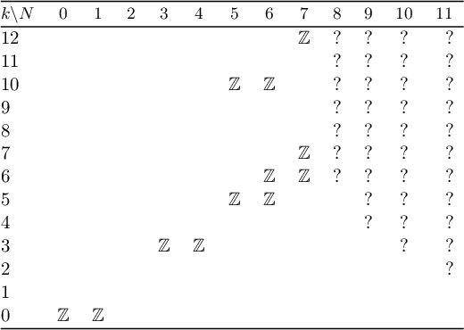
Adding this to the results of [Reference Elbaz-Vincent, Gangl and Soulé19], one obtains Table 5.
The groups
 $H_{k+N-1}({\mathrm {Vor}}_{\mathit {GL}_N(\mathbb{Z} )}) = H_k(\mathit {GL}_N(\mathbb{Z} );\mathrm {St}_N)$
modulo
 $\mathcal {S}_{N+1}$
. Empty slots denote
 $0$
.

5.3 Cohomology of modular groups
When
 $\Gamma =\mathit {SL}_N(\mathbb{Z} )$
or
 $\mathit {GL}_N(\mathbb{Z} )$
, we know
 $H^m(\Gamma ;\tilde{\mathbb{Z}} )$
by combining (4) (end of §1.2.3), Section 4.2 and (6). As shown above, this allows us to compute the cohomology of
 $\Gamma $
with trivial coefficients. The results are given in Corollary 5.2 below.
Corollary 5.2. From Borel–Serre duality, we have
 $$\begin{align*}H^{\frac{N(N-1)}{2}-k} (\mathit{GL}_N(\mathbb{Z}); \mathbb{Z})=0\quad \mod \mathcal{S}_{N+1}\, , \end{align*}$$
for
 $N=8,9,10,11$
and
 $0<k\leqslant 12-N$
.
Remark 5.3. This provides further evidence for a conjecture of Church, Farb and Putman [Reference Church, Farb and Putman11], see Conjecture 2.
6 Application to algebraic K-theory of integers
The homology of the general linear group with coefficients in the Steinberg module can also be used to compute the K-theory of
 $\mathbb{Z} $
. Let
 $P(\mathbb{Z} )$
be the exact category of free
 $\mathbb{Z} $
-modules of finite rank, let Q be the category obtained from
 $P(\mathbb{Z} )$
by applying Quillen’s Q-construction [Reference Quillen44], and let
 $BQ$
be its classifying space. Let
 $Q_N$
be the full subcategory of Q containing all free
 $\mathbb{Z} $
-modules of rank at most N and
 $BQ_N$
its classifying space. One of the definitions of the algebraic K-theory groups [Reference Quillen44] is
 $$\begin{align*}K_m (\mathbb{Z}) = \pi_{m+1} (BQ) \, , \quad m \geqslant 0 \,. \end{align*}$$
Therefore we can compute
 $K_m (\mathbb{Z} )$
if we understand the homology of
 $BQ$
as well as the Hurewicz map
 $$\begin{align*}h_m \colon K_m (\mathbb{Z}) \to H_{m+1} (BQ;\mathbb{Z}). \end{align*}$$
To do so, we use that Quillen proved in Theorem 3 of [Reference Quillen43] that there are long exact sequences

Since
 $BQ_0 \simeq \ast $
, these allow us to inductively obtain information about the homology of
 $BQ_N$
from
 $H_*(\mathit {GL}_N(\mathbb{Z} );\mathrm {St}_N)$
.
6.1 On the homology of
$BQ$

Using Proposition 1.5, we can rewrite the above Quillen sequences as

We obtain the following result concerning the homology of
 $BQ$
. It is proven using a spectral sequence, but a reader unfamiliar with spectral sequences may reproduce the results by inductively using the long exact sequences (8).
Proposition 6.1. Modulo
 $\mathcal {S}_7$
we have
 $$\begin{align*}H_m(BQ;\mathbb{Z}) = \begin{cases} 0 & \text{if } m=2,3,4,5,8,9 \\ \mathbb{Z} & \text{if } m=0,1,6,7,10,11.\end{cases}\end{align*}$$
Furthermore, modulo
 $\mathcal {S}_{11}$
we have
 $H_{12}(BQ;\mathbb{Z} ) = \mathbb{Z} $
.
Proof. The long exact sequences (8) give rise to a spectral sequence
 $$\begin{align*}E^1_{pq} = H_q(\mathit{GL}_p(\mathbb{Z});\mathrm{St}_p) \Longrightarrow H_{p+q}(BQ;\mathbb{Z}).\end{align*}$$
We shall use this modulo
 $\mathcal {S}_{7}$
and
 $\mathcal {S}_{11}$
respectively. Table 5 gives most of the
 $E^1$
-page for
 $p \leqslant 11$
and
 $q \leqslant 12$
, substituting
 $N=p$
and
 $k=q$
.
For
 $m \leqslant 12$
, the diagonal line
 $p+q=m$
contains either no non-zero entry, or a single entry
 $\mathbb{Z} $
. Thus to prove the first part, it suffices to show that the
 $d^1$
-differentials
 $d^1 \colon E^1_{p+1,q} \to E^1_{p,q}$
vanish modulo
 $\mathcal {S}_7$
for
 $p+q \leqslant 12$
. For the second part, we need to further verify that all
 $d^r$
-differentials
 $d^r \colon E^r_{6+r,6-r+1} \to E^r_{6,6}$
vanish modulo
 $\mathcal {S}_{11}$
. Since these are homomorphisms into abelian groups that are either zero or free, we can prove this by verifying it after tensoring with
 $\mathbb{Q} $
.
To do so, we use that the rational homotopy groups of
 $BQ$
are known by work of Borel, §12 of [Reference Borel5]:
 $$\begin{align*}\pi_m(BQ) \otimes \mathbb{Q} = \begin{cases} \mathbb{Q} & \text{if } m=1 \text{ or}, m = 4i+2 \text{ with } i \text{ a positive integer,} \\ 0 & \text{otherwise.}\end{cases}\end{align*}$$
Since
 $BQ$
is an infinite loop space, the rational homotopy groups determine its rational homology groups: for
 $m \leqslant 12$
,
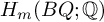 $H_m(BQ;\mathbb{Q} )$
is
 $0$
if
 $m=2,3,4,5,8,9$
and
 $\mathbb{Q} $
if
 $m = 0,1,6,7,10,11,12$
. This proves the desired statement.
Remark 6.2. That the coinvariants
 $H_0(\mathit {GL}_N(\mathbb{Z} );\mathrm {St}_N)$
vanish for
 $N \geqslant 3$
is due to Lee and Szczarba, Theorem 1.3 of [Reference Lee and Szczarba37]. They deduce this by exhibiting a generating set of
 $\mathrm {St}_N$
. In [Reference Church and Putman12], Church and Putman give a presentation of
 $\mathrm {St}_N$
, from which one may deduce that
 $H_1(\mathit {GL}_N(\mathbb{Z} );\mathrm {St}_N)=0$
modulo
 $\mathcal {S}_N$
for
 $N \geqslant 3$
. In fact, Theorem A of [Reference Church and Putman12] gives only a rational statement, but it is straightforward to verify their argument goes through modulo
 $\mathcal {S}_N$
. In [Reference Miller, Nagpal and Patzt42], Miller, Patzt and Nagpal have shown that
 $H_{1} (\mathit {SL}_N(\mathbb{Z} ); \mathrm {St}_N)= 0$
for
 $N \geqslant 6$
, that is, without needing to work modulo
 $\mathcal {S}_N$
. More recently, Brück, Miller, Patzt, Sroka and Wilson [Reference Brown8] proved a similar vanishing result (rationally) for
 $H_{2} (\mathit {SL}_N(\mathbb{Z} ); \mathrm {St}_N)$
and
 $N\geqslant 3$
.
6.2 On the Hurewicz homomorphism
By definition, for every integer
 $m \geqslant 1$
,
 $$\begin{align*}K_{m} (\mathbb{Z}) = \pi_{m+1} (BQ) \,. \end{align*}$$
The space
 $BQ$
is in fact
 $\Omega ^{\infty -1} \mathbf {K}(\mathbb{Z} )$
with
 $\mathbf {K}(\mathbb{Z} )$
the algebraic K-theory spectrum of
 $\mathbb{Z} $
, so in particular an infinite loop space. This has consequences for the kernel
 $C_m$
of the Hurewicz homomorphism
 $$\begin{align*}h_m \colon \pi_m (BQ) \to H_m (BQ;\mathbb{Z}) \,. \end{align*}$$
Proposition 6.3. Modulo
 $\mathcal {S}_5$
, we have
 $C_m = 0$
for
 $m=9,10,11$
. Modulo
 $\mathcal {S}_{7}$
, we have
 $C_{12}=0$
.
Proof. This follows from Theorem 1.5 of [Reference Arlettaz1], which implies that if X is a path-connected infinite loop space then the kernel of the Hurewicz homomorphism
 $\pi _n(X) \to H_n(X;\mathbb{Z} )$
is annihilated by
 $R_n$
, an integer divisible only by primes
 $\leqslant \frac {n}{2}+1$
. We apply this result to
 $X = BQ$
.
Theorem 6.4. The group
 $K_8 (\mathbb{Z} )$
is trivial.
Proof. From Propositions 6.1 and 6.3 we deduce that
 $K_8(\mathbb{Z} )=0$
modulo
 $\mathcal {S}_7$
. According to the Quillen–Lichtenbaum conjectures (see e.g. Chapter VI.10 of [Reference Weibel53]) if
 $\ell $
is a regular odd prime, there are no
 $\ell $
-torsion in
 $K_{2j}(\mathbb{Z} )$
for
 $j>0$
. Hence
 $K_8(\mathbb{Z} )=0$
.
Using an elaboration of the method presented, we can recover information about several related algebraic K-theory groups (see also Table VI.10.1.1 of [Reference Weibel53]).
Proposition 6.5. Modulo
 $\mathcal {S}_7$
,
 $K_9(\mathbb{Z} )\cong \mathbb{Z} $
and
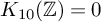 $K_{10}(\mathbb{Z} )=0$
. Modulo
 $\mathcal {S}_{11}$
,
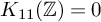 $K_{11}(\mathbb{Z} ) = 0$
.
Proof. Having proven Theorem 6.4, we know the groups
 $K_i(\mathbb{Z} )$
modulo
 $\mathcal {S}_7$
for
 $i \leqslant 8$
: they vanish unless
 $i=0,5$
in which case they are
 $\mathbb{Z} $
. The groups
 $K_i(\mathbb{Z} )$
are also the homotopy groups of the algebraic K-theory spectrum
 $\mathbf {K}(\mathbb{Z} )$
, and we conclude that there is a map of spectra
 $$\begin{align*}\mathbf{S}^0 \vee \mathbf{S}^5 \to \mathbf{K}(\mathbb{Z})\end{align*}$$
which is
 $8$
-connected modulo
 $\mathcal {S}_7$
. By the Hurewicz theorem modulo
 $\mathcal {S}_7$
, we see that
 $$\begin{align*}\pi_{10}(BQ) \cong H_{10}(BQ,\Omega^{\infty-1}(\mathbf{S}^0 \vee \mathbf{S}^5);\mathbb{Z})\end{align*}$$
modulo
 $\mathcal {S}_7$
. It is a standard computation that
 $H_{10}(\Omega ^{\infty -1}(\mathbf {S}^0 \vee \mathbf {S}^5);\mathbb{Z} ) = 0$
modulo
 $\mathcal {S}_7$
, so from Propositions 6.1 and the long exact sequence of a pair it follows that
 ${K_9(\mathbb{Z} ) = \pi _{10}(BQ) \cong \mathbb{Z} }$
modulo
 $\mathcal {S}_7$
.
This allows for the construction of a further map
 $$\begin{align*}\mathbf{S}^0 \vee \mathbf{S}^5 \vee \mathbf{S}^9 \to \mathbf{K}(\mathbb{Z})\end{align*}$$
which is
 $9$
-connected modulo
 $\mathcal {S}_7$
. Applying
 $\Omega ^{\infty -1}$
and repeating the above analysis in degrees
 $11$
and
 $12$
gives
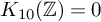 $K_{10}(\mathbb{Z} )=0$
modulo
 $\mathcal {S}_7$
and
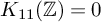 $K_{11}(\mathbb{Z} ) = 0$
modulo
 $\mathcal {S}_{11}$
.
Remark 6.6. As pointed out in Remark 6.2, [Reference Church and Putman12] proves that
 $H_1(\mathit {GL}_N(Z);\mathrm {St}_N)$
vanishes modulo
 $\mathcal {S}_{N}$
. In order to prove
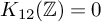 $K_{12}(\mathbb{Z} )=0$
, we thus ‘only’ need to recover the groups
 $H_{12}({\mathrm {Vor}}_{\mathit {GL}_N(\mathbb{Z} )})$
for
 $N=9,10,11$
which are still missing.
7 Arithmetic applications
For the convenience of the reader, we recall some facts about the relationship between algebraic K-theory and étale cohomology, with a view towards the Kummer–Vandiver conjecture. We follow the presentation of Kurihara [Reference Kurihara34] and Soulé [Reference Soulé49] (see also Section VI.10 of [Reference Weibel53]).
Let p be an odd prime,
 $i\in \mathbb{N} $
and
 $j\in \mathbb{Z} $
. Denote by

the étale cohomology groups of the scheme
 $\text {Spec}(\mathbb{Z} [1/p])$
with coefficients in the j-th Tate twist of the p-adic integers. It is known that when
 $j \neq 0$
these groups vanish unless
 $i=1,2$
. It was shown by Dwyer and Friedlander [Reference Dwyer and Friedlander17] and (independently) by Soulé [Reference Soulé48], that when
 $m=2j-i>1$
and
 $i=1,2$
, there is a surjective Chern map
 $$\begin{align*}K_m(\mathbb{Z}) \to H^i_{\text{\'et}}(\mathbb{Z}[1/p];\mathbb{Z}_p(j))\,. \end{align*}$$
Recall the following facts about these groups:
-
1. When
$p>j+1$
the groups
$H^1_{\text {\'et}}(\mathbb{Z} [1/p];\mathbb{Z} _p(j))$
vanish. -
2. When
$j>0$
is even, the order of
$H^2_{\text {\'et}}(\mathbb{Z} [1/p];\mathbb{Z} _p(j))$
is equal to the p-part of the numerator of
$B_j/j$
(this is a consequence of the ‘main Iwasawa’s conjecture’ [Reference Mazur and Wiles41], see [Reference Kurihara34] or [Reference Soulé49] for more details).





Hence, those groups are not known when
 $i=2$
and j is odd (assuming
 $p>j+1$
). At the level of m it means that m is divisible by 4. Let
 $\mathbb{Q} (\zeta _p)$
be the cyclotomic extension of
 $\mathbb{Q} $
obtained by adding p-th roots of unity. Let C be the p-Sylow subgroup of the class group of
 $\mathbb{Q} (\zeta _p)$
. The group
 $\Delta =\text {Gal}(\mathbb{Q} (\zeta _p)/\mathbb{Q} )\cong (\mathbb{Z} /p) ^{\times }$
acts upon C via the Teichmüller character
 $$\begin{align*}\omega \colon \Delta \to (\mathbb{Z}/p) ^{\times}\, ,\end{align*}$$
with
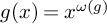 $g(x)=x^{\omega (g)}$
and
 $x^p=1$
. For all
 $i\in \mathbb{Z} $
let
 $$\begin{align*}C^{(i)} = \{ x \in C \quad\text{such that}\quad g(x)=\omega(g)^i x \quad \text{for all}\quad g\in \Delta\}\,. \end{align*}$$
Let
 $C^+$
be the subgroup of C fixed by the complex conjugation of
 $\mathbb{Q} (\zeta _p)$
. The Kummer-Vandiver conjecture states that
 $C^+=0$
for arbitrary p. By the above construction, it turns out that
 $C^+$
is the direct sum of the groups
 $C^{(i)}$
for i even and
 $0\leqslant i \leqslant p-3$
. We then deduce the reformulation of the Kummer–Vandiver conjecture [Reference Kurihara34, Reference Soulé49]:
Conjecture 7.1 (Kummer–Vandiver conjecture)
The groups
 $C^{(i)}$
vanish for i even and
 $0\leqslant i \leqslant p-3$
.
From op. cit., using the above setting, we get a surjective map
 $$\begin{align*}K_{2m-2}(\mathbb{Z}) \twoheadrightarrow C^{(p-m)}\,. \end{align*}$$
As consequence of (6.4), we get
Corollary 7.1. The groups
 $C^{(p-5)}$
are zero for all prime
 $p>3$
.
Remark 7.2. By [Reference Soulé49], we know that
 $C^{(p-n)}$
is zero for p ‘large enough’ with respect to n. From computations done by Buhler and Harvey [Reference Buhler and Harvey10], we know that the conjecture is true for all (irregular) primes
 $p<163 577 856$
. This was recently improved to
 $p<2 147 483 648$
by Hart, Harvey and Ong [Reference Hart, Harvey and Ong28].
Acknowledgments
Philippe Elbaz-Vincent is partially supported by the French National Research Agency in the framework of the Investissements d’Avenir programme (ANR-15-IDEX-02). Furthermore part of this work was done during his stay at the Hausdorff Research Institute for Mathematics during the trimester ‘Periods in Number Theory, Algebraic Geometry and Physics’. Alexander Kupers was supported by the Danish National Research Foundation through the Centre for Symmetry and Deformation (DNRF92) and by the European Research Council (ERC) under the European Union’s Horizon 2020 research and innovation programme (grant agreement No. 682922) and is currently supported by NSF grant DMS-1803766.
Competing interests
The author(s) declare none.
Data availability statement
The data that support the findings of this study are openly available at https://github.com/elbazvip/Voronoi-complexes-database.