





1. Introduction
In open-channel flow, the aspect ratio (defined as the ratio of channel width to flow depth  ) is a key parameter governing the velocity distribution and turbulence characteristics in the cross-section. At low
 , the flow exhibits significant time-averaged secondary currents (SCs) that enhance lateral and vertical momentum exchange, leading to the downward shift of maximum velocity from the water surface, a phenomenon known as the ‘velocity dip’. In contrast, at high
 , the velocity dip is absent, and in the vicinity of the channel’s centreline, the flow is considered to be two-dimensional, or one-dimensional in the case of uniform flow when velocity statistics of the flow depend on the distance from the bed only. Based on extensive experiments, Nezu et al. (Reference Nezu, Nakagawa and Tominaga1985) concluded that when
 the velocity dip is absent, a finding later confirmed by a large number of experimental and numerical investigations (Yang et al. Reference Yang, Tan and Lim2004; Knight et al. Reference Knight, Hazlewood, Lamb, Samuels and Shiono2018; Sakai Reference Sakai2019; Yu et al. Reference Yu, Modesti and Pirozzoli2023). Most studies focus on either low-
 (i.e.
 ) or high-
 (i.e.
 ) open-channel flows (OCFs), with the transitional range of
 covered in less detail.
The first definition and classification of SCs have been provided by Prandtl (Reference Prandtl1952), who identified three kinds of SCs depending on their origin and driving factors. One of them, known as SCs of the second kind, can be observed in straight open channels where SCs are generated due to turbulence anisotropy and heterogeneity (Einstein & Li Reference Einstein and Li1958). Subsequently, Hinze (Reference Hinze1967) interpreted SCs of the second kind from an energetic perspective, attributing their origin to the imbalance between turbulence production and dissipation in different flow regions, as follows from the turbulent kinetic energy equation. Further theoretical advances (e.g. Einstein & Li Reference Einstein and Li1958; Bradshaw Reference Bradshaw1987; Nezu Reference Nezu2005; Nikitin Reference Nikitin2021), through the analysis of the streamwise vorticity equation, clarified how turbulence anisotropy and inhomogeneity lead to the formation of SCs. These theoretical advances have stimulated extensive investigations on SCs in open channels and natural rivers (Nezu et al. Reference Nezu, Nakagawa and Tominaga1985; Grega et al. Reference Grega, Hsu and Wei2002; Broglia et al. Reference Broglia, Pascarelli and Piomelli2003; Joung & Choi Reference Joung and Choi2010; Nikora & Roy Reference Nikora and Roy2012; Yang et al. Reference Yang, Tan and Wang2012; Stoesser et al. Reference Stoesser, McSherry and Fraga2015; Sakai Reference Sakai2019; Nikitin et al. Reference Nikitin, Popelenskaya and Stroh2021), focusing on their structural features, generation mechanisms and impact on the flow dynamics.
Secondary currents in low- OCFs typically consist of a pair of counter-rotating vortices (Broglia et al. Reference Broglia, Pascarelli and Piomelli2003): a lower vortex (also referred to as the secondary cell) that transports fluid towards the wall–bed corner and an upper vortex that drives flow towards the water surface. This phenomenon was later confirmed by Nikitin et al. (Reference Nikitin, Popelenskaya and Stroh2021), who suggested that the (upper) cell near the water surface is more intense and attains velocities of up to 5 % of the bulk velocity (
 $U_b$
). The lower cell near the bed is weaker (
 $\approx 2.5\,\% U_b$
) as it is confined at the wall–bed corner. The geometry of the cross-section (Brosda & Manhart Reference Brosda and Manhart2022; Kadia et al. Reference Kadia, Lia, Albayrak and Pummer2024), the channel Reynolds number (Sakai Reference Sakai2019; Yu et al. Reference Yu, Modesti and Pirozzoli2023) and the aspect ratio (Sakai Reference Sakai2019; Yu et al. Reference Yu, Modesti and Pirozzoli2023) all influence the shape, size and intensity of these two time-averaged streamwise vortices. Recent direct numerical simulations (DNS) performed by Yu et al. (Reference Yu, Modesti and Pirozzoli2023) have further advanced the understanding of the characteristics of SCs across the ranges of aspect ratios (
 ) and Reynolds numbers (6000
 ${\sim}$
106 000). Their results demonstrated that a third time-averaged vortex structure emerges between the upper and lower cells at
 , and the strength of the SCs increases with Reynolds number. In addition, spatially heterogeneous bed roughness, such as streamwise ridges or alternating smooth–rough strips (Stoesser et al. Reference Stoesser, McSherry and Fraga2015; Vanderwel & Ganapathisubramani Reference Vanderwel and Ganapathisubramani2015; Zampiron et al. Reference Zampiron, Cameron and Nikora2020), can itself drive SCs of the second kind through spanwise gradients in turbulence anisotropy, thereby modifying, or even dominating, the cellular pattern otherwise set by the sidewalls.
The presence of SCs in low- OCFs leads to several subsequent alterations in the mean velocity distribution, including the aforementioned velocity dip phenomenon (Nezu et al. Reference Nezu, Nakagawa and Tominaga1985; Yang et al. Reference Yang, Tan and Lim2004; Knight et al. Reference Knight, Hazlewood, Lamb, Samuels and Shiono2018; Sakai Reference Sakai2019; Yu et al. Reference Yu, Modesti and Pirozzoli2023), a contribution from SCs to the channel’s friction (Pirozzoli Reference Pirozzoli2018; Liu et al. Reference Liu, Stoesser and Fang2022a
; Yu et al. Reference Yu, Modesti and Pirozzoli2023) and a non-uniform shear stress distribution along the bed and sidewalls (Brosda & Manhart Reference Brosda and Manhart2022; Liu et al. Reference Liu, Stoesser and Fang2022b
).
While in OCFs with  , SCs span the entire cross-section, they also occupy the near sidewall region in wide-channel flows (
 ) and are assumed to have a negligible effect on the time-averaged flow field in the centre of the channel (Nezu et al. Reference Nezu, Nakagawa and Tominaga1985; Nezu & Nakagawa Reference Nezu and Nakagawa1993; Nikora & Roy Reference Nikora and Roy2012). It is perceived wisdom that for
 , the mean flow in the channel centre is primarily governed by wall-induced turbulence, for instance, in the form of persistent instantaneous counter-rotating vortical structures that generate alternating high- and low-speed streaks, known as very-large-scale motions (VLSMs). This turbulence feature has received increasing attention recently (e.g. Hutchins & Marusic Reference Hutchins and Marusic2007; Adrian & Marusic Reference Adrian and Marusic2012; Cameron et al. Reference Cameron, Nikora and Stewart2017).
The initial identification of VLSMs in wall-bounded flows has emerged from pipe flow study by Kim & Adrian (Reference Kim and Adrian1999), who identified coherent structures with streamwise wavelengths of
 $12{-}14$
pipe radii, in addition to large-scale structures with wavelengths around 2 pipe radii. Since then, they have often been termed VLSMs and large-scale motions (LSMs). Compared with pipes, ducts or boundary-layer flows (Guala et al. Reference Guala, Hommema and Adrian2006; Balakumar & Adrian Reference Balakumar and Adrian2007), the manifestation of VLSMs in OCFs exhibits distinctly varying scales. In smooth-bed OCFs, Duan et al. (Reference Duan, Chen, Li and Zhong2020, Reference Duan, Zhong, Wang, Zhang and Li2021) and Peruzzi et al. (Reference Peruzzi, Poggi, Ridolfi and Manes2020) reported wavelengths of VLSMs of approximately
 $20h{-}40h$
, which are comparable to those in flows in pipes and ducts. The VLSMs have been shown to contribute substantially to turbulent statistics in OCFs, accounting for approximately
 $40\,\%{-}50\,\%$
of the streamwise velocity variance and approximately
 $20\,\%{-}30\,\%$
of the Reynolds shear stress (Duan et al. 2020, 2021). Flume experiments by Peruzzi et al. (Reference Peruzzi, Poggi, Ridolfi and Manes2020) provided initial insights into VLSMs in OCFs with different aspect ratios, ranging from
 = 3.05 to 12.2. Their results suggested, rather unexpectedly, that VLSMs occur in the central part of the channel even at the lowest aspect ratio investigated (
 ). However, the wavelength of VLSMs in a channel with
 is significantly smaller than those observed in the wider-channel flow cases (
 ).
For rough-bed OCFs, the VLSM’s streamwise dimension ranges within
 $20{-}50$
flow depths, depending on bed roughness type, aspect ratio and the water depth-to-roughness-height ratio (Cameron et al. Reference Cameron, Nikora and Stewart2017; Cerino et al. Reference Cerino, Zampiron, Proust, Berni and Nikora2024; Zampiron et al. Reference Zampiron, Cerino, Berni, Proust and Nikora2024b
). Cameron et al. (Reference Cameron, Nikora and Stewart2017) demonstrated that, whereas the wavelength of LSMs scale with the flow depth, the wavelength of VLSMs in rough-bed OCFs do not scale purely with the flow depth but additionally depend on the channel width, roughness height and viscous scales. In particular, their data exhibited an apparent negative correlation between the friction Reynolds number (
 $\textit{Re}_{\tau }$
) and the VLSMs’ wavelength. However, by incorporating additional rough-bed experimental datasets (Zampiron et al. Reference Zampiron, Cameron and Nikora2020; Shen et al. Reference Shen, Yang and Liu2023; Cerino et al. Reference Cerino, Zampiron, Proust, Berni and Nikora2024), Cerino et al. (Reference Cerino, Zampiron, Proust, Berni and Nikora2024) identified a further trend in VLSM wavelength that was independent of
 $\textit{Re}_{\tau }$
, suggesting that
 $\textit{Re}_{\tau }$
is unlikely to be the primary parameter governing VLSM wavelength. More recently, Jing et al. (Reference Jing, Duan, Li, Cao and Zhu2025) showed that the contributions of both LSMs and VLSMs to the mean wall-shear stress are lower in rough-bed OCFs than in their smooth-bed counterparts at comparable Reynolds numbers, attributing this reduction to the suppression of LSMs by SCs induced by the rough wall.
The VLSMs are perceived as elongated instantaneous turbulence structures (sometimes referred to as streaks) with prominent counter-rotating streamwise vortices, which are similar to instantaneous SCs (e.g. Cameron et al. Reference Cameron, Nikora and Stewart2017; Zampiron et al. Reference Zampiron, Cerino, Berni, Proust and Nikora2024b
). This topological similarity has motivated extensive research into their interaction. Earlier observations suggested a mutually supportive relationship: e.g. Nugroho et al. (Reference Nugroho, Hutchins and Monty2013) and Kevin et al. (Reference Kevin, Monty, Bai, Pathikonda, Nugroho, Barros, Christensen and Hutchins2017) argued that roughness-induced SCs arise from a preferential alignment of VLSMs enforced by bed heterogeneity. More recent numerical and laboratory studies, however, argue that these two motion modes compete for kinetic energy and therefore cannot coexist. Yao et al. (Reference Yao, Chen and Hussain2018) reported that the energy-containing motions in channel flow are markedly weakened when strong SCs are imposed, similar to later observations in OCF of Peruzzi et al. (Reference Peruzzi, Poggi, Ridolfi and Manes2020). Liu et al. (Reference Liu, Stoesser and Fang2022a
) likewise showed that prominent SCs in partially filled pipe flows suppress VLSMs, which are present in fully filled pipe flows at the same Reynolds number where SCs are essentially absent. For OCFs over streamwise-aligned ridges, Zampiron et al. (Reference Zampiron, Cameron and Nikora2020) showed that VLSMs are completely suppressed whenever the ridge spacing is
 ${\leq} 2h$
. In addition, Zampiron et al. (Reference Zampiron, Cameron and Nikora2020) introduced the term secondary current instability (SCI) to describe a peak in the pre-multiplied velocity spectra with a wavelength of
 $3h{-}6h$
, i.e. at a scale intermediate between LSMs (
 $2h{-}3h$
) and VLSMs (
 $20h{-}50h$
). They demonstrated that the SCI absorbs energy from VLSMs, thus limiting their formation. Luo et al. (Reference Luo, Stoesser, Cameron, Nikora, Zampiron and Patella2023) subsequently revealed that ridge-induced SCI grows and decays quasi-periodically.
So far, evidence that SCs inhibit the formation of VLSMs has been gathered under geometric conditions that result in strong SCs, whether through pronounced topographic heterogeneity (Zampiron et al. Reference Zampiron, Cameron and Nikora2020; Liu et al. Reference Liu, Stoesser and Fang2022a; Luo et al. Reference Luo, Stoesser, Cameron, Nikora, Zampiron and Patella2023) or artificial body forcing (Yao et al. Reference Yao, Chen and Hussain2018). In conventional OCF over a homogeneous bed surface, by contrast, near sidewall SCs generated at bed-sidewall and water-surface–sidewall corners are weaker than under the aforementioned conditions. The research reported here employs the method of large-eddy simulation to study flows in smooth-bed OCFs with aspect ratios varying between  and
 . Bed and sidewall roughness are not considered in this study, while the friction Reynolds numbers are maintained within a narrow range to minimise their potential influence on SCs/SCIs, LSMs and VLSMs. The main goal of the reported study is thus to clarify modifications in the flow structure induced by the transition from conditions of narrow-channel flow (
 ) to wide-channel flow (
 ). To achieve this goal, we attempt to clarify (i) whether temporal manifestation of sidewall-induced SCs develops quasi-periodic instabilities (i.e. SCIs); (ii) how far SCs/SCIs extend away from the sidewalls in wider-channel flows; (iii) the potential coexistence of SCs/SCIs, LSMs and VLSMs in narrow and wide OCFs, as well as the threshold of
 for such coexistence; and (iv) the dynamic interrelations between SCs/SCIs, LSMs and VLSMs in wide OCFs.
The remainder of this manuscript is organised as follows: the numerical framework is outlined in § 2, and then the numerical set-up and boundary conditions are explained in § 3. Statistical parameters of velocity fields are examined in §§ 4.1 and 4.2 to identify and quantify sidewall-induced SCs. In §§ 4.3 and 4.4, the existence of SCIs and the critical  threshold for VLSM existence are investigated through instantaneous flow patterns and pre-multiplied spectra. Then, the relationship between SCs/SCIs and VLSMs is explored with the help of phase-averaged velocities (§ 4.5). Finally, the conclusions are given in § 5.
2. Numerical framework
In this study, the method of large-eddy simulation (LES), using the code Hydro3-D, is employed to simulate turbulent flows in open channels with different aspect ratios. Hydro3-D has been validated and applied to several flows of similar complexity to the one reported here (Liu et al. Reference Liu, Stoesser, Fang, Papanicolaou and Tsakiris2017; McSherry et al. Reference McSherry, Chua, Stoesser and Mulahasan2018; Liu et al. Reference Liu, Fang, Huang and He2019; Ouro & Stoesser Reference Ouro and Stoesser2019; Liu et al. Reference Liu, Stoesser and Fang2022a ). The code employs a local mesh refinement (LMR) that further enhances its capability in resolving multi-scale turbulence efficiently (Cevheri & Stoesser Reference Cevheri and Stoesser2018). The code solves the filtered Navier–Stokes equations for incompressible, unsteady, and viscous flow on a staggered Cartesian grid
 \begin{equation} \displaystyle \frac {\partial u_i}{\partial x_i}=0, \end{equation}
 \begin{equation} \displaystyle \frac {\partial u_i}{\partial t}+\displaystyle \frac {\partial u_iu_j}{\partial x_j}=-\displaystyle \frac {1}{\rho }\frac {\partial p}{\partial x_i}+\displaystyle \frac {\partial (2\nu S_{ij})}{\partial x_j}-\displaystyle \frac {\partial \tau _{ij}}{\partial x_j}, \end{equation}
where
 $u_i$
and
 $u_j$
are spatially resolved velocity vectors (
 $i$
or
 $j$
= 1, 2 and 3 represent
 $x\text{-}$
,
 $y\text{-}$
,
 $z\text{-}$
axis directions, respectively), and similarly,
 $x_i$
,
 $x_j$
represent the spatial location vectors in the three directions;
 $\rho$
is the density of water,
 $p$
is the spatially resolved pressure,
 $\nu$
is kinematic viscosity and
 $S_{ij}=1/2(\partial u_i/\partial x_j+\partial u_j/\partial x_i)$
denotes the filtered strain-rate tensor. The subgrid-scale (SGS) stress
 $\tau _{ij}$
is defined as
 $\tau _{ij}=-2\nu _tS_{ij}$
and in this study, the wall-adapting local eddy viscosity model proposed by Nicoud & Ducros (Reference Nicoud and Ducros1999) is used to approximate the SGS stresses. This model recovers the correct near-wall behaviour of the eddy viscosity without a wall-damping function and vanishes at the solid–water interface, which makes it suitable for the LES used here. The eddy viscosity is calculated as
 \begin{equation} \nu _t={(C_\omega \Delta )^2\frac {(s_{ij}^ds_{ij}^d)^{3/2}}{(S_{ij}S_{ij})^{5/2}+(s_{ij}^ds_{ij}^d)^{5/4}}}, \end{equation}
where
 $C_\omega$
is a constant with a value of 0.46 and
 $\Delta =(\Delta x\Delta y\Delta z)^{1/3}$
. The filtered traceless symmetric part of the square of the velocity gradient tensor is computed in the following form:
 \begin{equation} s_{ij}^d=\frac {1}{2}(g_{ik}g_{kj}+g_{jk}g_{ki})-\frac {1}{3}\delta _{ij}g_{kk}^2 \quad \text{ with } \quad g_{ij}=\frac {\partial u_i}{\partial x_j}. \end{equation}
The convection and diffusion terms of the Navier–Stokes equations are approximated by fourth-order accurate central differences. An explicit three-step Runge–Kutta scheme is used to integrate the equations in time, providing second-order accuracy. A fractional step method is employed, i.e. within the time step, convection and diffusion terms are solved explicitly first in a predictor step, which is then followed by a corrector step, during which the pressure and divergence-free velocity fields are obtained via a Poisson equation. The latter is solved iteratively using a multi-grid procedure (Cevheri & Stoesser Reference Cevheri and Stoesser2018; Ouro et al. Reference Ouro, Stoesser and Ramírez2018; Ouro & Stoesser Reference Ouro and Stoesser2019). The LMR algorithm allows for block-wise refinement of the computational grid, with a refinement ratio of 2 : 1 across neighbouring blocks. This facilitates finer grid resolution in regions of interest (e.g. near walls) while maintaining coarser resolution in less active regions. The LMR ensures accurate communication of variables across coarse–fine block interfaces through prolongation (interpolation) and restriction (averaging) procedures. Velocities in ghost cells on fine grids are obtained via quadratic interpolation constrained by mass conservation, and coarse ghost velocities are computed by averaging the fine-grid values. Pressure communication across block interfaces is handled using an approximate projection method based on interpolated pressure gradients. These procedures collectively preserve second-order spatial accuracy even in the presence of non-uniform grid transitions, as demonstrated by verification using the Taylor–Green vortex benchmark (Cevheri & Stoesser Reference Cevheri and Stoesser2018).
Flow parameters of the simulations:
 $u_*$
, friction velocity based on the mean pressure gradient;
 $U_b$
, bulk flow velocity;
 $\textit{Re}_h=U_b h/\nu$
, Reynolds number based on water depth;
 $\textit{Re}_R=U_b R_h/\nu$
, Reynolds number based on hydraulic Radius;
 $\textit{Re}_*=u_*h/\nu$
, friction Reynolds number;
 $N_x,N_y,N_z$
, number of grids in each direction;
 $\Delta x_f^+, \Delta y_f^+, \Delta z_f^+$
, normalised near-wall grid resolutions in each direction; cases EXP and DNS denote the experimental data by Duan et al. (Reference Duan, Chen, Li and Zhong2020) and the DNS of idealised, spanwise periodic two-dimensional OCF by Yao et al. (Reference Yao, Chen and Hussain2022);
 $^a$
, the friction velocity in the EXP is determined based on the log law.

Table 1 Long description
The table presents flow parameters of various simulations, including friction velocity, bulk flow velocity, Reynolds numbers, grid resolutions, and normalized near-wall grid resolutions. It has 7 rows and 12 columns. Column headers are: Case, B (cm), Re_h, Re_R, u_* (cm s^-1), u_*/U_b, Re_*, N_x x N_y x N_z, Δx_f^+, Δy_f^+, Δz_f^+, and Symbol. Row labels are: AR23, AR46, AR86, AR129, EXP, DNS. Each row provides specific values for each parameter. Notable trends include variations in grid resolutions and Reynolds numbers across different cases.
3. Set-up and boundary conditions
In this study,
 $x$
,
 $y$
and
 $z$
denote the streamwise, spanwise and vertical directions, respectively; the corresponding velocity components are
 $u$
,
 $v$
and
 $w$
. The coordinate system follows the standard left-handed convention, with the origin located at the intersection of the inlet plane, the channel bed and the left sidewall. Consequently, the
 $x$
-axis points downstream, the
 $z$
-axis points vertically upward and the
 $y$
-axis points towards the right sidewall. Table 1 provides the main hydraulic parameters of the simulation scenarios. In total, four simulations with a range of aspect ratios (
 ) are performed, notated as ‘AR’ followed by
 values (e.g. AR86). Case AR86 is designed to reproduce the dimensional conditions of the experiment of Duan et al. (Reference Duan, Chen, Li and Zhong2020), with
 $h=3.52$
cm,
 $U_b=59.4$
cm s
 $^{-1}$
and
 $B=30$
cm. Consequently, the Reynolds number based on water depth, i.e.
 $\textit{Re}_h=U_bh/\nu =20\,905$
, is identical to that in the smooth-bed experiment of Duan et al. (Reference Duan, Chen, Li and Zhong2020), allowing for validation of the LES approach. The LESs of the AR86 case are conducted using streamwise domain lengths of
 $L_x \approx 80h$
and
 $42h$
. The resulting premultiplied spectra of the streamwise velocity fluctuations are highly consistent (Appendix A; figure 20), indicating that
 $L_x \approx 42h$
is sufficient to capture the most dynamically relevant flow structures at
 . It should be noted that this domain length may be insufficient for cases with larger aspect ratios. Nevertheless, to ensure computational feasibility and consistency across all cases,
 $L_x=42h$
is adopted throughout, which falls within the range commonly used in previous LES and DNS studies of VLSMs in OCFs (e.g. Pinelli et al. Reference Pinelli, Herlina, Wissink and Uhlmann2022; Yao et al. Reference Yao, Chen and Hussain2022; Bauer et al. Reference Bauer, Sakai and Uhlmann2025). For the other cases,
 $h$
and
 $U_b$
are kept unchanged, while only the channel width varies (
 $B=8$
,
 $16$
and
 $45$
cm for AR23, AR46 and AR129, respectively). Owing to the difference between hydraulic radius (
 $R_h$
) and flow depth at low aspect ratios, the Reynolds numbers based on hydraulic radius,
 $\textit{Re}_R=U_b R_h/\nu$
, are also reported in table 1, spanning
 $\textit{Re}_R \approx 11\,100{-}18\,100$
. The friction Reynolds number (
 $\textit{Re}_*$
) in table 1 is defined as
 $\textit{Re}_*=u_*h/\nu$
, where
 $u_*$
is the bulk friction velocity obtained from the mean pressure gradient (
 $\text{d}p/\text{d}x$
) as
 $u_*=\sqrt {-(R_h/\rho )(\text{d}p/\text{d}x)}$
in the LES. The streamwise pressure gradient, which is equivalent to the channel slope in a laboratory flume, is determined dynamically during the simulation. Specifically, the pressure gradient is adjusted to maintain the time-averaged inlet velocity at the prescribed target value
 $U_b$
. Therefore,
 $u_*$
is not prescribed but obtained from the computed pressure gradient, explaining the small differences in
 $u_*/U_b$
among the cases. In the experiment of Duan et al. (Reference Duan, Chen, Li and Zhong2020),
 $u_*$
is determined based on the log law, yielding a
 ${\sim} 5\,\%$
lower
 $u_*/U_b$
than that in case AR86. Re-evaluating the friction velocity as
 $u_*=\sqrt {ghS}$
from the reported bed slope (
 $S$
), water depth and gravitational acceleration (
 $g$
) in Duan et al. (Reference Duan, Chen, Li and Zhong2020) gives
 $u_*/U_b=0.053$
, very close to the value in AR86. A periodic boundary condition is employed in the streamwise direction, and no-slip boundary conditions are applied at the side and bottom walls. At the top boundary, a rigid lid is assumed by applying a free-slip boundary condition. The accuracy of this approximation is evaluated through an additional simulation for case AR46 that resolves the deformed water surface, denoted AR46-LSM. The comparison shows that the free-slip boundary condition preserves the overall SC sizes and positions, while modestly affecting the magnitude of the surface vortex and the turbulence statistics in the immediate near-surface region. Full details of the set-ups and results for case AR46-LSM are provided in Appendix B.
Computational mesh for the AR46 simulation (every fifth grid point shown).
 $(a)$
Cross-sectional (
 $y$
–
 $z$
) mesh, with the locally refined near-wall blocks (black) and the coarsened outer block (red), illustrating the wall-normal grid stretching;
 $(b)$
schematic of a near-wall grid cell showing its aspect ratio (
 $\Delta x_f = 2.5\Delta y_f \approx 3.0\Delta z_f$
) and the near-wall resolution in wall units (
 $\Delta x_f^+ = 10.2$
,
 $\Delta y_f^+ = 4.09$
,
 $\Delta z_f^+ = 3.27$
).

Calculations are carried out on a mesh of
 $2400\times 176$
grid points for all cases in the streamwise (
 $x$
) and vertical (
 $z$
) directions, respectively, with the number of grid points increasing from 320 to 1800 in the spanwise (
 $y$
) direction as the aspect ratio increases from 2.3 to 12.9. Locally refined meshes are applied to all cases. Figure 1 shows an example of the mesh used in case AR46. A fine mesh (
 $\Delta x_{f}$
,
 $\Delta y_{f}$
,
 $\Delta z_{f}$
) is employed near both bottom and sidewalls, extending over an identical wall-normal distance of 0.5
 $h$
. In the outer regions, a coarsened mesh (
 $\Delta x_{c}$
,
 $\Delta y_{c}$
,
 $\Delta z_{c}$
) with grid spacing twice that of the fine mesh in all three directions is used. Both fine and coarse meshes are stretched, with a grid aspect ratio
 $\Delta x=2.5\Delta y\approx 3.0\Delta z$
. Given that a staggered grid is used for velocity and pressure, the near-wall grid resolution for the first streamwise velocity grids is defined as
 $\Delta ^+=0.5 u_*\Delta _f/\nu$
. Consequently, the largest near-wall grid resolutions are
 $\Delta x^+_{f}=10.2,\Delta y^+_{f}=4.09, \Delta z^+_{f}=3.27$
, respectively. These grid resolutions are also comparable to those adopted in previously reported high-resolution LES studies (
 $z^+\lt 4$
in Mathieu et al. (Reference Mathieu, Chauchat, Bonamy, Balarac and Hsu2021) and
 $z^+\lt 5$
in Liu et al. (Reference Liu, Stoesser and Fang2022a
)). Details of the grid sizes and resolutions are provided in table 1. Compared with the Kolmogorov dissipative length scale (
 $\eta$
), the current grid spacings range from
 $\Delta x_f/\eta \approx 8.0$
,
 $\Delta y_f/\eta \approx 3.2$
and
 $\Delta z_f/\eta \approx 2.6$
near the upper boundary of the viscous sublayer, to
 $\Delta x_c/\eta \approx 4.9$
,
 $\Delta y_c/\eta \approx 2.0$
and
 $\Delta z_c/\eta \approx 1.6$
in the fully turbulent region (Appendix C). This suggests the LES successfully resolves absolute majority of turbulent eddies, from those comparable to the simulation domain size to those where viscosity start to dominate over inertia.
All simulations are initially run for 10 flowthroughs (FTs), defined as
 $FT=L_x/U_b$
, to establish fully developed turbulence, and then are continued for another 40 FTs to collect sufficient data for turbulence statistics. Velocity data are recorded at four longitudinal planes located at
 $y/h$
= 0.5, 1.0, 2.0 and at the channel centreline (
 $y/B$
= 0.5), as well as at a cross-section at
 $x/h$
= 20.0. All data are sampled at a frequency of 100 Hz for subsequent analysis. In the following, the overline symbol
 $\bar {\boldsymbol{\cdot }}$
indicates time averaging, and angular brackets with a subscript
 $\langle \boldsymbol{\cdot }\rangle _{x}$
or without subscripts
 $\langle \boldsymbol{\cdot }\rangle$
denote spatial averaging in the streamwise direction or in both the streamwise and vertical directions, respectively. The superscript
 $\boldsymbol{\cdot }^{+}$
represents a quantity that is normalised by the friction velocity and fluid viscosity, e.g.
 $\langle \bar {u}\rangle _x^+=\langle \bar {u}\rangle _x/u_*$
for the streamwise velocity,
 $z^+=zu_*/\nu =(z/h)\textit{Re}_*$
for the vertical distance and
 $u_{\mathit{rms}}^{+} = \langle \overline {u'^2}\rangle _x^{0.5}/u_*$
for the root-mean-square of the streamwise velocity fluctuations.
Profiles of
 $(a)$
the time-averaged streamwise velocity, (
 $b$
) the root-mean-square of the streamwise velocity fluctuation and (
 $c$
) the root-mean-square of the vertical velocity fluctuation at the channel centreline for the
 case, together with the DNS results of Yao et al. (Reference Yao, Chen and Hussain2022) and the experimental data of Duan et al. (Reference Duan, Chen, Li and Zhong2020).

4. Results and discussions
4.1. Validation
Figure 2 presents profiles of
 $(a)$
the normalised streamwise velocity
 $\langle \bar {u}\rangle _x^+$
,
 $(b)$
the root-mean-square streamwise velocity fluctuations
 $u_{\mathit{rms}}^+$
and
 $(c)$
the root-mean-square vertical velocity fluctuation
 $w_{\mathit{rms}}^+$
at the channel centreline (
 $y/B=0.5$
) in the
 channel as predicted by the LES, together with DNS (Yao et al. Reference Yao, Chen and Hussain2022) and experimental (Duan et al. Reference Duan, Chen, Li and Zhong2020) data. The mean velocity profile predicted by the LES agrees very well with both the DNS and experimental profiles, all showing features typical of canonical wall-bounded turbulence, with a viscous sublayer at
 $z^+\lt 5$
, a buffer layer within
 $5\lt z^+\lt 100$
and a logarithmic layer at
 $z^+\gt 100$
(Marusic et al. Reference Marusic, McKeon, Monkewitz, Nagib, Smits and Sreenivasan2010). In addition, the LES-predicted streamwise and vertical velocity fluctuations (figure 2
 $b{,}c$
) peak at
 $z^+\approx 15$
and
 $z^+\approx 100$
, respectively, which is comparable to other wall-bounded turbulent flows (e.g. Monty et al. Reference Monty, Hutchins, Ng, Marusic and Chong2009; Marusic et al. Reference Marusic, McKeon, Monkewitz, Nagib, Smits and Sreenivasan2010; Lee & Moser Reference Lee and Moser2015). For the velocity fluctuations, the LES results agree well with both the DNS and experimental data in terms of the overall distribution, although the magnitudes of the
 $ u_{\mathit{rms}}^+$
and
 $w_{\mathit{rms}}^+$
peaks show minor differences between LES and EXP, that are within
 $10\,\%$
. Overall, the close agreement among LES, DNS and experiments supports the validity of the present LES approach.
4.2. Mean flow structure
Profiles of the normalised streamwise time-averaged velocity
 $(a)\,\langle \bar {u}\rangle ^+$
, and root-mean-square of velocity fluctuations:
 $(b)\,u_{\mathit{rms}}^+$
,
 $(c)\,v_{\mathit{rms}}^+$
and
 $(d)\,w_{\mathit{rms}}^+$
at the centreline for the four
 cases. The grey dashed and dashed-dot lines in panel
 $(a)$
denote the linear law
 $u^+=z^+$
and the logarithmic law
 $u^+=(1/\kappa )\ln (z^+)+A$
, respectively, where
 $\kappa =0.39$
is the von Kármán constant and
 $A=4.6$
, following Yao et al. (Reference Yao, Chen and Hussain2022).

Figure 3 shows profiles of
 $(a)$
the normalised streamwise velocity
 $\langle \bar {u}\rangle _x^+$
, and the root-mean-square velocity fluctuations:
 $(b)\,u_{\mathit{rms}}^+$
,
 $(c)\,v_{\mathit{rms}}^+$
and
 $(d)\,w_{\mathit{rms}}^+$
along the respective channel centreline for the four simulation cases (table 1). The time-averaged velocity profiles collapse onto each other in the inner regions (
 $z^+\lt 400$
), while the ‘velocity dip’ is significant in the AR23 case near the water surface and completely disappears in the AR86 and AR129 cases (figure 3
 $a$
). These findings align well with the early experimental observations in OCFs reported by Nezu et al. (Reference Nezu, Nakagawa and Tominaga1985), who pointed out that the velocity dip is absent in channels with
 . Regarding the turbulent fluctuations, the vertical distances (
 $z^+$
) for the peaks of the three components are almost the same across the four cases, with their values decreasing as
 increases from 4.6 to 12.9. This is attributed to the decline in turbulent kinetic energy (TKE) production at higher
 , as shown in figure 4. However, case AR23 exhibits a different trend, having a smaller maximum compared with AR46 in all three fluctuation components due to lower TKE production (figure 4
 $c$
) with respect to that in AR46. Figure 4(
 $a$
) demonstrates that the differences in the vertical velocity gradient remain invisible across all cases, while the peak of Reynolds shear stress in case AR23 is approximately 10 % lower than in AR46 (figure 4
 $b$
). Consequently, in the AR23 case, the attenuation of the Reynolds shear stress directly dictates the net reduction in TKE production (figure 4
 $c$
). It is also noted that
 $u_{\mathit{rms}}^+$
and
 $v_{\mathit{rms}}^+$
increase at larger
 $z^+$
in the immediate vicinity of the free surface. This is attributed to the slightly higher TKE convection and turbulent transport in the spanwise direction very close to the water surface (not shown for brevity).
Profiles of (
 $a$
) the vertical gradient of the time- and streamwise-averaged velocity,
 $\partial \langle \overline {u}\rangle _x/\partial z$
, normalised by
 $u_*/h$
, (
 $b$
) the Reynolds shear stress,
 $-\langle \overline {u'w'} \rangle$
, normalised by
 $u_*^2$
and (
 $c$
) the TKE production,
 $\langle \textit{TKE}_p \rangle =-\langle \overline {u'w'}\rangle \times ({\partial \langle \overline {u}\rangle _x}/{\partial z})$
, normalised by
 $u_*^3/h$
, along the channel centreline for the four
 cases. The legends are the same as in figure 3.

Contours of the time- and streamwise-averaged velocity normalised by the bulk velocity
 $\langle \overline {u}\rangle _x/U_b$
for
 $(a)$
AR23,
 $(b)$
AR46,
 $(c)$
AR86,
 $(d)$
AR129. The solid lines represent the velocity maximum lines.

Contours of the time- and streamwise-averaged velocity,
 $\langle \overline {u}\rangle _{x}/U_b$
, are shown in figure 5. For cases AR46, AR86 and AR129, the deviations in
 $\langle \overline {u}\rangle _{x}/U_b$
between any two symmetric positions relative to the channel centreline are less than
 $1\,\%$
, confirming the inherent symmetry of the flow about the channel centreline and that the level of data convergence is sufficient. Therefore, only half of the cross-section is presented in figure 5 and subsequent figures except AR23. For case AR23, the maximum velocity occurs approximately
 $0.3h$
below the water surface at the centreline. This dip distance is slightly smaller than those reported for OCFs with
 : for example, Nezu et al. (Reference Nezu, Nakagawa and Tominaga1985) and Yu et al. (Reference Yu, Modesti and Pirozzoli2023) provided values of approximately
 $0.368h$
and
 $0.35h$
, respectively. Given a negative correlation between dip distances and
 demonstrated by Yu et al. (Reference Yu, Modesti and Pirozzoli2023) and the slightly larger aspect ratio in case AR23, the location of the velocity dip observed here is considered consistent with previous studies. The isolines in the vicinity of the bottom wall bisector bulge downwards, a result of the bottom corner vortex, which is consistent with the conventional knowledge (e.g. Prandtl Reference Prandtl1952) and recent DNS at
 of Yu et al. (Reference Yu, Modesti and Pirozzoli2023). For higher
 cases, the velocity dip at the channel centreline disappears, yet the bulging towards the corners still exists. Following Nezu et al. (Reference Nezu, Nakagawa and Tominaga1985), a velocity maximum line,
 $z_{\textit{max}}/h$
, at which
 $\langle \overline {u}\rangle _{x}/U_b$
attains its maximum at each lateral position, is examined and shown as solid lines in figure 5. The profiles of these maximum velocity lines for each case are nearly the same against the distance from the sidewall (
 $y/h$
). For instance, the profile of AR129 is nearly identical to that of AR86, and both coincide with AR46 up to
 $y/h=2.3$
. The shapes and lateral extents of these maximum velocity lines agree with those reported by Nezu et al. (Reference Nezu, Nakagawa and Tominaga1985) at comparable aspect ratios (e.g. a lateral extent of approximately
 $2.5h$
at
 compared with
 $2.46h$
in case AR86).
Contours of the time- and streamwise-averaged secondary flow strength normalised by the bulk velocity
 $U_s/U_b$
for
 $(a)$
AR23,
 $(b)$
AR46,
 $(c)$
AR86,
 $(d)$
AR129. The time-averaged secondary flow vectors are superimposed for all cases.

Figure 6 presents contours of the normalised time- and streamwise-averaged secondary flow strength,
 $U_s/U_b$
for the four
 cases. Here, the secondary flow strength is calculated as
 $U_s=\sqrt {\langle \overline {v}\rangle _{x}^2+\langle \overline {w}\rangle _{x}^2}$
(Liu et al. Reference Liu, Stoesser and Fang2022a
). Vectors of the time-averaged secondary flow are also added, with a reference vector of magnitude
 $0.05U_b$
. The two prominent corner vortices are observed in all four cases, i.e. one near the water surface (hereafter referred to as the surface vortex, SV) and the other near the sidewall–bed corner (hereafter referred to as the bottom vortex, BV). The BV is similar in size and strength regardless of the aspect ratio and is confined within
 $y/h\lt 0.8$
and
 $z/h\lt 0.6$
, with a maximum
 $U_s$
of approximately
 $2.5\,\%U_b$
, which is consistent with previous findings (Nezu et al. Reference Nezu, Nakagawa and Tominaga1985; Sakai Reference Sakai2019; Yu et al. Reference Yu, Modesti and Pirozzoli2023). By contrast, the size of the SV in cases AR46, AR86, AR129 is substantially larger than that in case AR23, attaining a spanwise width of roughly 2.3
 $h$
. This agrees with the OCF measurements at
 reported by Nezu et al. (Reference Nezu, Nakagawa and Tominaga1985) and Onitsuka & Nezu (Reference Onitsuka and Nezu2001). Meanwhile, the secondary flow is strongest in case AR23 (figure 6
 $a$
) among all cases, where the maximum SC strength reaches
 $U_s/U_b\approx 0.065$
at the water surface, similar to values previously reported for narrow OCFs (Liu et al. Reference Liu, Stoesser and Fang2022a
; Yu et al. Reference Yu, Modesti and Pirozzoli2023), and consistent with laboratory experiments of Tominaga et al. (Reference Tominaga, Nezu, Ezaki and Nakagawa1989), Nezu & Nakagawa (Reference Nezu and Nakagawa1993) and Zampiron et al. (Reference Zampiron, Cameron and Nikora2020). In addition, a weak vortex spanning the entire water depth is observed at
 $y/h \approx 2.7$
in the wide channels, cases AR86 and AR129 (figure 6
 $c$
,
 $d$
). A similar secondary flow was also identified in OCF at
 $y/h \approx 2.5$
with
 by Nezu et al. (Reference Nezu, Nakagawa and Tominaga1985). In the two wide cases, SCs are absent near the channel centreline, in agreement with the absence of the velocity dip in figure 5(c,d). As demonstrated by simulations with a free surface in Appendix B, the topology and position of the SV remain robust, although the free-slip boundary condition modestly underestimates its maximum strength.
Contours of the normalised spanwise shear stress for
 $(a)$
AR23,
 $(b)$
AR46,
 $(c)$
AR86,
 $(d)$
AR129 in the cross-section. Vectors denote the time-averaged secondary flow.

In order to further elucidate the role of SCs in transporting turbulent momentum, the contours of the normalised Reynolds shear stresses
 $-\overline {u'v'}$
and
 $-\overline {u'w'}$
are examined, and these are presented in figures 7 and 8. The highest (absolute) values of
 $-\overline {u'v'}$
are observed near the sidewalls in all cases. The BV exerts a marked influence on
 $-\overline {u'v'}$
, characterised by a minimum of
 $-\overline {u'v'}$
in the centre of the BV. Additionally, a region of elevated levels of
 $-\overline {u'v'}$
appears on the side of the vortex away from the sidewall, located at
 $y/h \approx 0.8$
in the
 case and
 $y/h \approx 1$
in the other cases. These regions behave as turbulent shear zones that induce localised velocity reduction (figure 5). Similar moderate
 $-\overline {u'v'}$
regions and corresponding velocity reductions were also reported in the DNS by Yu et al. (Reference Yu, Modesti and Pirozzoli2023). In contrast,
 $-\overline {u'v'}$
remains consistently low throughout the region influenced by the SV, with normalised values of
 $-\overline {u'v'}/u_*^{2} \approx 0.2$
. In cases AR86 and AR129, the weak depth-spanning SC near
 $y/h = 2.7$
gives rise to a zone of slightly negative
 $-\overline {u'v'}$
spanning the entire water column.
The distribution of
 $-\overline {u'w'}$
is primarily characterised by a vertical gradient, modulated by local perturbations due to the SCs near the sidewalls. In regions dominated by the SV, a zone of negative
 $-\overline {u'w'}$
emerges, spanning the entire channel width in AR23 and extending to approximately
 $y/h = 2.1$
away from the walls in the other cases. The presence of a near-surface region of negative
 $-\overline {u'w'}$
reflects the presence of a velocity maximum below the water surface (figure 5), the spanwise line of which serves as a separation line between positive and negative Reynolds stresses
 $-\overline {u'w'}$
. Near the wall–water-surface corner, a very small area of positive
 $-\overline {u'w'}$
is observed, consistent with observations in partially filled pipes (Brosda & Manhart Reference Brosda and Manhart2022) and narrow open channels (Yu et al. Reference Yu, Modesti and Pirozzoli2023). Furthermore, the BV generates a localised hump in
 $-\overline {u'w'}$
near the bed, located at
 $y/h \approx 0.7$
in case AR23 and
 $y/h \approx 1.0$
in the other cases. The co-occurrence of elevated
 $-\overline {u'v'}$
and
 $-\overline {u'w'}$
at these locations indicates strong turbulence production driven by LSMs, as is discussed further in § 4.4.
Contours of the normalised vertical shear stress for
 $(a)$
AR23,
 $(b)$
AR46,
 $(c)$
AR86,
 $(d)$
AR129 in the cross-section. The solid lines represent the
 $\overline {u'w'}=0$
.

4.3. Instantaneous flow
Contours of the normalised streamwise velocity fluctuations in a horizontal (
 $x{-}y$
) plane at
 $z/h=0.5$
for various aspect ratios are presented in figure 9, illustrating qualitative differences in the coherence of velocity fields. The full channel width is shown here, since the instantaneous field is not symmetric about the centreline. As the streaks meander and evolve in time, these snapshots serve only to illustrate the structures qualitatively. In the cases with
 and
 $8.6$
(figure 9
 $d{,}c$
), elongated, meandering streaks of alternating high- and low-momentum fluid, which typically correspond to VLSMs, are clearly visible. These structures resemble those reported in previous studies of turbulent boundary layers and OCFs (e.g. Hutchins & Marusic Reference Hutchins and Marusic2007; Cameron et al. Reference Cameron, Nikora and Stewart2017; Zampiron et al. Reference Zampiron, Cameron and Nikora2020). In contrast, the contours in the
 case show little evidence of VLSMs. In the
 case, visualised structures appear to be longer than in the narrowest-channel flow, with some strong low-momentum streaks present in the vicinity of the channel centre (e.g. in the range
 $x/h=20{-}35$
), with associated high-momentum streaks being somewhat weaker. The length scale of the streaks in the channels with
 cannot be reliably determined from the instantaneous flow fields alone, and therefore, spectral analysis is employed in the following section to quantitatively characterise the structures’ dominant wavelengths.
Contours of the instantaneous normalised streamwise velocity fluctuation at
 $z/h=0.5$
over the full channel width in channels with
 $(a)$
AR23,
 $(b)$
AR46,
 $(c)$
AR86,
 $(d)$
AR129.

4.4. Spectral characteristics
Contours of pre-multiplied spectra of streamwise velocity fluctuations for the four cases at increasing distance from the sidewall: (
 $a,c,f,j$
)
 $y/h=0.5$
, (
 $b,d,g,k$
)
 $y/h=1.0$
, (
 $e,h,l$
)
 $y/h=2.0$
and (
 $i,m$
)
 $y/B=0.5$
(channel centreline). Peaks in the spectra are highlighted as: solid line denoting LSMs, long-dash line denoting VLSMs and dash-dotted line denoting SCI. Where
 $k_x=2\pi /\lambda _x$
is the streamwise wavenumber,
 $\varPhi _{uu}$
is the velocity spectrum. Values of
 $k_x\varPhi _{uu}/u_*^2\lt 0.1$
are masked.

Pre-multiplied spectra of the streamwise velocity component,
 $k_x\varPhi _{uu}/u_*^2$
, where
 $k_x=2\pi /\lambda _x$
is the streamwise wavenumber and
 $\lambda _x$
is the corresponding wavelength (e.g. Kim & Adrian Reference Kim and Adrian1999; Hutchins & Marusic Reference Hutchins and Marusic2007; Monty et al. Reference Monty, Hutchins, Ng, Marusic and Chong2009), are computed using instantaneous velocities in longitudinal planes (
 $x{-}z$
planes) at spanwise distances
 $y/h$
= 0.5, 1.0, 2.0 and
 $y/B=0.5$
away from the sidewall. Note that the spectra for the
 $y/B=0.5$
plane are calculated only for the cases AR86 and AR129. Approximately 1000 instantaneous snapshots are collected at uniform time interval in each of the longitudinal planes. The spectra are initially obtained for each time instant and subsequently ensemble averaged to produce the smoothed spectral contours presented in figure 10. For
 $y/h=0.5$
and
 $ z/h \lt 0.6$
(figure 10
 $a{,} c{,} h{,} j$
), which corresponds to the region occupied by the BV (figure 7
 $a{-}d$
), all cases exhibit a spectral peak at approximately
 $\lambda _x\approx 6h$
. Therefore, this wavelength is likely to be associated with SCI, as defined in Zampiron et al. (Reference Zampiron, Cameron and Nikora2020). Noticeably, the wavelength of the SCI appears to be larger than that of the LSMs (solid lines), i.e.
 $\lambda _x\approx 3h$
for all cases in figure 10 (
 $b{,} d{,} g{,} k$
). It is hypothesised that the spectral peak at
 $\lambda _x\approx 6h$
represents an instability associated with sidewall-generated SCs, and more evidence of this SCI is provided in § 4.5. At
 $y/h=0.5$
, another region of elevated
 $k_x\varPhi _{uu}/u_*^2$
emerges at
 $z/h\gt 0.8$
. Its characteristic wavelengths are identified with the aid of figure 22 in Appendix D, in which
 $k_x\varPhi _{uu}$
is normalised by the
 $z$
-dependent streamwise Reynolds normal stress. Figure 22 shows that the dominant wavelengths range from approximately 3
 $h$
–4
 $h$
and decrease with distance from the free surface, down to
 $z/h\approx 0.7$
. Within
 $0.6\lesssim z/h\lesssim 0.7$
, a deficit in the pre-multiplied spectral energy is observed in the
 $y/h=0.5$
plane. This deficit is likely associated with the reduced TKE production there (Appendix E; figure 23). Conversely, the TKE production rate increases toward the free surface (figure 23), further supporting the elevated
 $k_x\varPhi _{uu}/u_*^2$
observed at
 $z/h\gt 0.8$
(figure 10
 $a{,} c{,} h{,} j$
).
For  , another spectral peak emerges at approximately
 $\lambda _x\approx 20h$
at
 $y/h=0.5$
, suggesting that VLSMs extend into this near-sidewall region. These signatures may arise either from the local generation of VLSMs independently of the SCIs or from the sidewall-ward transport of VLSMs generated near the channel centre. Future investigations are required to assess the relative importance of these two mechanisms. The wavelengths of the SCI and VLSMs agree with what was observed in OCFs recently. For example, wavelengths of VLSMs reported in Zampiron et al. (Reference Zampiron, Cameron and Nikora2020) and Duan et al. (Reference Duan, Chen, Li and Zhong2020) are
 $\lambda _x=19.7{-}25.3h$
and
 ${\approx} 20h$
, respectively, with more similar estimates given in a recent summary on VLSM wavelengths in smooth-bed OCFs in Cerino et al. (Reference Cerino, Zampiron, Proust, Berni and Nikora2024). The wavelengths of SCIs found by Zampiron et al. (Reference Zampiron, Cameron and Nikora2020) and Luo et al. (Reference Luo, Stoesser, Cameron, Nikora, Zampiron and Patella2023) are
 $\lambda _x=2.7{-}5h$
and
 $4{-}10h$
, respectively, which are consistent with the current estimate.
Away from the sidewalls (figure 10
 $e{,} h{,} i{,} l{,} m$
), the maximum values in the velocity spectra near the water surface gradually diminish, accompanied by an expansion of the high-energy regions near the bed. The high-energy VLSM regions reach almost to the water surface, most noticeably at the channel centreline for the
 case. The spectral signatures of SCIs become insignificant in planes with
 $y/h \ge 1.0$
across all cases. Instead, a shorter wavelength peak (the solid lines) emerges in these planes. This spectral peak represents the LSMs originating from the bottom walls, with a typical wavelength (
 $\lambda _x\approx 3h$
) similar to those reported for OCFs (e.g. Cameron et al. Reference Cameron, Nikora and Stewart2017) and other wall-bounded flows (Kim & Adrian Reference Kim and Adrian1999; Hutchins & Marusic Reference Hutchins and Marusic2007; Smits et al. Reference Smits, McKeon and Marusic2011). It is also noteworthy that the wavelength of VLSMs in the AR46 case is approximately
 $10h$
at
 $y/h=2$
, which is nearly half of that for the large
 cases. A similar trend is also reported by Peruzzi et al. (Reference Peruzzi, Poggi, Ridolfi and Manes2020), who found that the VLSM wavelength in OCFs at
 (also
 ${\sim} 10h$
) is approximately half of that at
 .
Pre-multiplied spectra of streamwise velocity at fixed vertical locations at (
 $a$
)
 $z/h=0.2$
, (
 $b$
)
 $z/h=0.5$
, (
 $c$
)
 $z/h=0.75$
, (
 $d$
)
 $z/h=0.9$
for four cases, spectra for successive
 are offset vertically by
 $0.5$
(
 $0.3$
in panel
 $c$
). The dashed and solid lines denote the spectra based on velocities at
 $y/h = 0.5$
and the channel centreline, respectively, for all four cases. The legends are the same as in figure 3.

In figure 11, pre-multiplied spectra at various elevations including (
 $a$
)
 $z/h=0.2$
, (
 $b$
)
 $z/h=0.5$
, (
 $c$
)
 $z/h=0.75$
, (
 $d$
)
 $z/h=0.9$
are plotted for the four cases. The solid and dashed lines represent spectra at the channel centreline and near the sidewall (
 $y/h=0.5$
), respectively. At low elevations (
 $z/h = 0.2$
, figure 11
 $a$
), the spectral energy in the channel centre is higher than near the sidewall across all ARs. This arises from stronger turbulence production due to higher near-bed velocity gradients (figure 5) and higher Reynolds shear stress (figure 8). However, at the highest elevation (
 $z/h=0.9$
, figure 11
 $d$
), this trend reverses: the turbulent energy near the sidewall noticeably exceeds that in the centre, suggesting intensified streamwise fluctuations near the water surface driven by SCs. For the sidewall spectra, the dominant wavelength is
 $\lambda _x\approx 6h$
across most
 and elevations, except at
 $z/h=0.2$
in AR23 and at
 $z/h=0.75$
, where the peak is less distinct. Whereas for the centreline spectra, VLSMs with
 $\lambda _x \approx 20h$
are identified at all elevations for the two higher
 cases, although the peak becomes broader and weaker towards the free surface. At
 , large-wavelength peaks are noticeable within
 $z/h \le 0.5$
(figure 11
 $a$
,
 $b$
), but the wavelength is approximately
 $10h$
. There are also LSMs signatures in the pre-multiplied spectra in the channel centre, especially visible in the near-bed region of flow cases with larger aspect ratios.
Spanwise variation of pre-multiplied spectra of streamwise velocity fluctuation at three wall-normal elevations:
 $(a,d,g,j)$
 $z/h=0.2$
,
 $(b,e,h,k)$
 $z/h=0.5$
and
 $(c,f,i,l)$
 $z/h=0.8$
, with rows corresponding to AR23, AR46, AR86 and AR129, respectively. The solid, dash-dotted and dashed lines denote the LSMs, SCIs and VLSMs respectively. The solid and dashed lines originate at
 $y/h=3.0$
and extend towards the sidewall, whereas the dash-dotted lines originate at the sidewall and extend towards the channel centre. The spanwise extent of each line is determined by its intersection with the isoline corresponding to a
 $z/h$
-dependent threshold of
 $k_x\varPhi _{uu}/u_*^2$
. The threshold values are set to
 $k_x\varPhi _{uu}/u_*^2$
=
 $0.7$
,
 $0.4$
and
 $0.2$
at
 $z/h=0.2$
,
 $z/h=0.5$
,
 $z/h=0.8$
, respectively. Values of
 $k_x\varPhi _{uu}/u_*^2\lt 0.1$
are masked.

Figures 10 and 11 suggest a progressive transition in the dominant motions from SCIs near the sidewalls to VLSMs toward the channel centre in cases with  . To further elucidate the spanwise organisation of energetic motions, figure 12 presents the pre-multiplied spectra of streamwise velocity as functions of the streamwise wavelength
 $\lambda _x/h$
and the spanwise coordinate
 $y/h$
at three representative vertical locations (
 $z/h = 0.2$
,
 $0.5$
and
 $0.8$
). This analysis reveals the lateral distributions of the energy of velocity fluctuations and their characteristic wavelengths across the channel width. Unlike figures 10 and 11, where spectra are computed in the streamwise wavenumber domain, the data in figure 12 are obtained in the frequency domain. Using the 40 FT velocity time series collected at
 $x/h=10.0$
, the frequency spectra are obtained at uniform spatial intervals defined by the background (coarse) grid resolution (i.e. at every two grid points in the cross-section). To convert frequency to streamwise wavelengths, Taylor’s frozen-turbulence hypothesis is employed using
 $\lambda _x=\langle \overline {u}\rangle _x/f$
, where
 $f$
is the frequency. The applicability of this conversion is assessed in Appendix F (figure 24), where direct comparisons with spatial spectra show close agreement over the energy-containing wavelength range, thereby validating the use of Taylor’s hypothesis.
At all vertical locations and across all cases, the pre-multiplied spectra exhibit a clear two-zone lateral structure, consisting of a near-sidewall region and a region farther from the sidewall. A transient zone at
 $y/h \approx 0.2-0.4$
of reduced spectral energy separates these two regions. Near the bed (figure 12
 $a$
,
 $d$
,
 $g$
,
 $j$
), the near-sidewall spectral zone remains confined within
 $y/h \le 0.2$
and shows no distinct energetic wavelengths. In contrast, SCI-associated wavelengths (
 $\lambda _x/h \approx 6$
, dash-dotted circles) appear as a local spectral bulge within
 $0.3 \le y/h \le 0.6$
for all cases. Farther away from the sidewall, the dominant spectral energy shifts to the LSM-associated scale (solid lines),
 $\lambda _x/h \approx 3$
. At half-water depth (
 $z/h$
= 0.5 in figure 12
 $b$
,
 $e$
,
 $h$
,
 $k$
), the lateral arrangement of the LSM-associated wavelength bands resembles that observed near the bed, albeit with overall reduced spectral energy. For AR86 and AR129, an additional spectral feature emerges at
 $y/h \gtrsim 2.1$
, i.e. spectral hills at wavelengths at
 $\lambda _x/h \approx 20$
, corresponding to VLSMs. However, the SCI-associated bulges within
 $0.3 \le y/h \le 0.6$
disappear. Concurrently, a new
 $ \lambda _x/h \approx 6$
spectral ridge develops adjacent to the sidewall and extends to
 $y/h \lesssim 0.4$
(figure 12
 $b$
,
 $e$
,
 $h$
,
 $k$
). The lateral extension of this ridge and the spectral energy remain at the highest elevation
 $z/h$
= 0.8 (figure 12
 $c$
,
 $f$
,
 $i$
,
 $l$
), indicating a consistent SCI zone at
 $z/h\gt 0.5$
near the sidewall. In addition, the LSM band weakens substantially at
 $z/h=0.8$
and no longer forms a distinct spectral peak (a weak LSM signature nonetheless persists, e.g. in AR86), so no LSM line is drawn at this elevation; the VLSM footprints, by contrast, remain noticeable.
Spanwise distributions of the normalised pre-multiplied streamwise velocity spectra for
 $(a)$
AR23,
 $(b)$
AR46,
 $(c)$
AR86 and
 $(d)$
AR129. For each case, the upper and lower subpanels show depth averaging over the sampled elevations within the upper (
 $0.6\lt z/h\lt 1$
) and lower (
 $0.1\lt z/h\lt 0.6$
) depth ranges, respectively. The orange solid and magenta dash-dotted lines denote the spectral energy evaluated at
 $\lambda _x=3h$
(LSM scale) and
 $\lambda _x=6h$
(SCI scale), respectively. The cyan dashed lines denote the long-wavelength contribution evaluated at
 $\lambda _x/h=10$
for AR23 and AR46 and at
 $\lambda _x/h=20$
for AR86 and AR129.

To quantitatively determine the locations of transitions among SCIs, LSMs and VLSMs, figure 13 presents the spanwise distributions of the pre-multiplied spectra averaged separately over the lower layer (
 $0.1\lt z/h\lt 0.6$
) and the upper layer (
 $0.6\lt z/h\lt 1$
). The spectra are evaluated at three selected wavelengths, i.e. at
 $\lambda _x/h = 3.0$
(
 $\langle k_x\varPhi _{uu}\rangle _z|_{\lambda _x=3h}$
),
 $\lambda _x/h = 6.0$
(
 $\langle k_x\varPhi _{uu}\rangle _z|_{\lambda _x=6h}$
) and
 $\lambda _x/h =$
10.0 (
 $\langle k_x\varPhi _{uu}\rangle _z|_{\lambda _x=10h}$
in AR23 and AR46) or 20.0 (
 $\langle k_x\varPhi _{uu}\rangle _z|_{\lambda _x=20h}$
in AR86 and AR129). These wavelength-dependent pre-multiplied spectra represent the contributions of LSMs, SCIs and VLSMs to the streamwise velocity fluctuations at different spanwise locations and vertical regions. Across all cases, the spectral energy averaged over
 $z/h\lt 0.6$
is generally higher than that averaged over
 $z/h\gt 0.6$
, particularly in the channel centre region, as TKE is primarily produced near beds (figures 4
c and 23). The contribution of VLSMs is markedly lower than that of LSMs and SCIs at both
 $z/h\lt 0.6$
and
 $z/h\gt 0.6$
across all spanwise locations in AR23 (figure 13
 $a$
), within
 $y/h\lt 0.6$
in AR46 (figure 13
 $b$
) and within
 $y/h\lesssim 2.4$
in AR86 and AR129 (figure 13
 $c$
,
 $d$
). Beyond
 $y/h=0.6$
, the contribution at
 $\lambda _x/h=10$
becomes roughly comparable to those at the LSM- and SCI-associated wavelengths in AR46. Whereas, in AR86 and AR129, the spectral energy at
 $\lambda _x/h=20$
exceeds that of the other two since
 $y/h \approx 2.4$
. While the spectral magnitudes of LSMs and SCIs are comparable at
 $z/h\gt 0.6$
across all cases (the upper layer in figure 13(a–d)). Their relative energy contributions exhibit a spanwise dependence at
 $z/h\lt 0.6$
(the lower layer). Near the wall–bed corner (
 $y/h\lt 0.5$
and
 $z/h\lt 0.6$
in AR23 and
 $y/h\lt 0.6$
and
 $z/h\lt 0.6$
in the other three cases), the SCI-associated spectral energy is slightly higher than the LSM- and VLSM-associated contributions across all cases. Beyond
 $y/h\approx 0.6$
, the LSM-associated contribution becomes slightly higher than that of SCI until the VLSM-associated contribution becomes increasingly important. Taken together, figures 12 and 13 establish a consistent picture in which the organisation of energetic turbulent motions transitions from a SCI-dominated near-sidewall dynamics to LSM- and ultimately VLSM/LSM-dominated behaviour, particularly at
 $z/h\lt 0.6$
.
4.5. Phase-averaged statistics
In order to visualise flow features that correspond to the respective turbulence structures, SCIs and VLSMs, a phase-averaging procedure is applied to the velocities in the cross-section (Luo et al. Reference Luo, Stoesser, Cameron, Nikora, Zampiron and Patella2023; Tang et al. Reference Tang, Stoesser, Huang, Liu and Fang2025). The procedure involves (i) subtracting the local time-averaged streamwise velocity from the instantaneous velocity to obtain the streamwise velocity fluctuation and applying a Gaussian filter to the streamwise velocity fluctuation at selected locations, (ii) identifying local maxima and minima of the filtered fluctuation signal and their corresponding frequencies, (iii) dividing a maximum-minimum-maximum cycle into six phases (snapshots) by six equal time intervals and (iv) calculating the respective phase-averaged velocity in the entire cross-section (Appendix G). The phase-averaged velocity fluctuations are denoted as
 $\dot {u}'$
,
 $\dot {v}'$
and
 $\dot {w}'$
. Figure 14 shows an example of the raw and Gaussian filtered streamwise velocity fluctuation
 $(a)$
at the centre of BV (
 $y/h=0.5$
and
 $z/h=0.2$
) and
 $(b)$
at the channel centreline (
 $y/B=0.5$
and
 $z/h=0.2$
) in case AR86 and their respective velocity spectra (
 $c$
) and (
 $d$
). The grey dashed lines in figures 14
 $(a)$
and 14
 $(b)$
are two sinusoidal curves with wavelengths of
 $\lambda _x/h=6$
and
 $\lambda _x/h=20$
, respectively. The Gaussian filter is applied to remove the LSM-scale and smaller-scale fluctuations, so that the SCI (and the VLSM at the centreline) can be reliably identified and used as the phase reference. The width (i.e. standard deviation) of the Gaussian filter is chosen to be
 $0.6h$
. The velocity spectra of the original and Gaussian-filtered signals (figure 14
 $c{,}d$
) show that the spectral density of LSMs (
 $fh/U_b \approx 0.33$
) reduces by approximately one order of magnitude, while the spectral densities of SCI and VLSMs are largely retained (
 $fh/U_b \le 0.16$
). For the SCI (figure 14
 $a$
), a total of 480 local maxima and minima (blue open symbols) are identified during the
 ${\sim} 40$
FT duration data (only the first 10 FT of data are shown in figure 14), yielding a periodicity of
 $\langle \overline {u}\rangle _{x}\Delta t=6h$
(in other words,
 $\lambda _x/h=6$
), while for the VLSMs, 84 cycles are identified (figure 14
 $b$
), corresponding to a wavelength of approximately
 $20h$
. The number of cycles identified for the other three cases (not shown for brevity) also agrees with the corresponding wavelengths in figure 10. At the centre of BV, all cases exhibit a range of 155–240 cycles. At the channel centreline, case AR23 detects 87 cycles, while cases AR46 and AR129 show 88 and 85 cycles, respectively.
The LES-computed and Gaussian-filtered velocity signals for case AR86
 $(a)$
at the centre of the BV and
 $(b)$
in the channel centreline, at the same level as in
 $(a)$
. Power spectral density (PSD) of the streamwise velocity fluctuation
 $(c)$
at the centre of the BV and
 $(d)$
in the channel centreline for the same case. The grey dashed lines are sinusoidal reference curves with wavelengths of
 $\lambda _x/h=6$
in (
 $a$
) and
 $\lambda _x/h=20$
in (
 $b$
).

Figure 15 illustrates the phase-averaged in-plane velocity vectors (
 $\dot {v}, \dot {w}$
), defined as
 $\dot {v}=\dot {v}'+\overline {v}$
and
 $\dot {w}=\dot {w}'+\overline {w}$
, together with the phase-averaged streamwise velocity fluctuation (
 $\dot {u}'$
) of case AR46. The first column in figure 15 shows results obtained by applying phase averaging at the centre of BV, whereas the second column corresponds to phase averaging at the channel centreline. The instantaneous centres of the BV and SV are marked by red and blue dots, respectively, in the first column. The inset in figure 15
 $(a)$
shows the BV-centre positions over all phases and clearly reveals a clockwise, periodic back-and-forth cycling motion. When
 $\dot {u}$
at
 $y/h = 0.5$
,
 $z/h = 0.2$
reaches its maximum (figure 15
 $a$
), the BV centre is farthest from the sidewall at
 $y/h = 0.58$
, and the vortex reaches its maximum size, extending to approximately
 $y/h \approx 1.0$
and
 $z/h \approx 0.6$
. Owing to this enlarged BV, high-momentum fluid from the outer layer is entrained downward towards the bed along the bed–sidewall corner bisector, producing a region of positive
 $\dot {u}'$
in the left part of the BV. Meanwhile, low-momentum fluid near the corner is ejected upward around
 $y/h \approx 1.0$
. Thereafter, the BV contracts and its centre shifts towards the corner region, reaching a minimum position at
 $y/h = 0.34$
with its size shrinking to nearly half (figure 15
 $d$
). At this phase,
 $\dot {u}$
reaches its minimum and the surrounding streamwise velocity is uniformly reduced (
 $\dot {u}'\lt 0$
). Notably, the velocity on the right side of the BV increases because of the influx of high-momentum fluid from the SV (figure 15
 $c{,}d$
). As the cycle progresses, a re-expansion of the BV and a retreat of its centre away from the sidewall during the ascending half of the
 $\dot {u}$
cycle occurs. The vertical displacement of the BV centre is relatively small, approximately one third of its maximum spanwise displacement.
Contours of the phase-averaged streamwise velocity fluctuation deduced from Gaussian-filtered velocity signals and vectors of the secondary flow (
 $\dot {v}/U_b, \dot {w}/U_b$
) in case AR46. Panels
 $(a{-}f)$
and
 $(g{-}l)$
are the six successive phases (equal time intervals over one cycle), with
 $(a)$
at the maximum and
 $(d)$
at the minimum, of the phase averaging at the centre of BV and at the channel centreline, respectively. The movement of the corner SC cell centre within one period of SC meandering is shown in an insert in
 $(a)$
.

The cycling motion of the BV induces a corresponding division–fusion cycle in the SVs. In figure 15 (
 $a{,}b{,}e{,}f$
) (where they exhibit relatively large
 $\dot {v}$
and
 $\dot {w}$
from the bed to the channel centre), two distinct SVs emerge: an inner SV at
 $y/h \approx 0.5$
and an outer SV at
 $y/h \approx 1.3$
. This likely arises because the enlarged BV occupies a substantial near-sidewall space, limiting the development of a large single SV and resulting in two smaller, spatially constrained vortices. In contrast, when BV contracts (figure 15
 $c{,}d$
) and releases space for SV development, the inner and outer SVs merge into one single, larger SV, whose size and shape resemble the time-averaged SV in figure 6. The clockwise, periodic back-and-forth cycle of the BV and its associated division–fusion cycle in the SVs described above appear again in higher
 cases (e.g. in AR86; figure 16). This finding suggests the ubiquitous occurrence of these two cycles in wide rectangular open channels. Furthermore, near the sidewall at
 $y/h \approx 0.2$
and
 $z/h \gtrsim 0.5$
, a local region of streamwise velocity fluctuations with an opposite sign to that of the instantaneous BV core is observed (figure 15
 $a{,}d$
and 16
 $a{,}d$
).
Contours of the phase-averaged streamwise velocity fluctuation deduced from Gaussian-filtered velocity signals and vectors of the secondary flow (
 $\dot {v}/U_b, \dot {w}/U_b$
) in case AR86. Panels
 $(a{-}f)$
and
 $(g{-}l)$
are the six successive phases (equal time intervals over one cycle), with
 $(a)$
at the maximum and
 $(d)$
at the minimum, of the phase averaging at the centre of BV and at the channel centreline, respectively. The movement of corner SC cell centre within one period of SC meandering is shown in an insert in
 $(a)$
.

Contours of the phase-averaged streamwise velocity fluctuation deduced from Gaussian-filtered velocity signals and vectors of the secondary flow (
 $\dot {v}/U_b, \dot {w}/U_b$
) in case AR23. Panels
 $(a{-}f)$
and
 $(g{-}l)$
are the six successive phases (equal time intervals over one cycle), with
 $(a)$
at the maximum and
 $(d)$
at the minimum, of the phase averaging at the centre of BV and at the channel centreline, respectively. The movement of corner SC cell centre within one period of SC meandering is shown in an insert in
 $(a)$
.

When examining the phase-averaged velocities at the centreline (figure 15
 $g{-}l$
), instantaneous near-bed vortices are observed only in phases of maximum (figure 15
 $g$
) and minimum (figure 15
 $j$
) velocities. When
 $\dot {u}$
at the centreline is near its peak, intensified downward motion transports high-momentum fluid towards the bed, giving rise to a pair of counter-rotating vortices near the sampling point (
 $y/B = 1/2$
,
 $z/h = 0.2$
). This vortex pair produces a region of positive
 $\dot {u}'$
flanked by two zones of negative
 $\dot {u}'$
. In contrast, at the minimum phase of
 $\dot {u}$
, a new pair of counter-rotating vortices forms with a reversed sense of rotation. These vortices jointly induce an upward flow near the sampling point, resulting in
 $\dot {u}'$
distributions of opposite sign compared with those at the maximum velocity phase. The remaining four phases represent transitional states between the velocity maximum and minimum phases, characterised by the absence of near-bed vortices and reduced zones of elevated
 $\dot {u}'$
. In AR46, the vortex pairs in figure 15(
 $g{,}j$
) occupy only approximately half of the water depth due to the persistent presence of SV. At higher AR, these pairs span almost the entire water depth (figure 16
 $g{,}j$
) and are also present in some of the transient stages (figure 16
 $h{,}l$
).
Figure 15 suggests that the SCI of BV is associated with periodic oscillations of its position and size, while the VLSMs at the channel centreline are linked to the formation and decay of two pairs of counter-rotating vortices with opposite senses of rotation. The SVs, especially the outer SV, are influenced by both mechanisms, thereby forming an indirect link between the SCI and VLSMs. This linkage is absent at higher  (figure 16) and strengthens at
 . For example, the minimum
 $\dot {u}$
phases at the BV centre (figure 17
 $d{,}e$
) share similar secondary vortices with the maximum
 $\dot {u}$
phases at the centreline (figure 17
 $g{,}h$
): (i) small and near-sidewall BV, (ii) strong downward motion near the centreline, (iii) an additional near-bed vortex adjacent to the BV and (iv) zones of negative and positive
 $\dot {u}'$
around
 $y/h$
= 0.5 and
 $y/h$
= 1.0, respectively.
To further investigate the spatial coherence of these flow structures, two-point correlations of the streamwise velocity fluctuations are computed as
 \begin{equation} R_{uu}(y_r,z_r,\Delta y,\Delta z) = \frac {\overline {u'(y_r,z_r)u'(y_r+\Delta y,z_r+\Delta z)}}{u_{\mathit{rms}}(y_r,z_r) u_{\mathit{rms}}(y_r+\Delta y,z_r+\Delta z)}, \end{equation}
where
 $(y_r,z_r)$
denotes the location of reference points. Figure 18 presents the contours of
 $R_{uu}$
with reference points chosen at the centre of the BV (reference points at
 $y/h=0.5$
,
 $z/h=0.2$
; panels
 $a,c$
) and at the channel centreline (reference points at
 $y/B=0.5$
,
 $z/h=0.2$
; panels
 $b,d$
). Focusing on the sidewall region (figure 18
 $a{,}c$
), the correlation map reveals a strong positive core coincident with the BV, flanked by regions of negative correlation. Crucially, a distinct region of negative correlation is observed adjacent to the sidewall (
 $y/h\lt 0.3,z/h\gt 0.5$
), with their locations coincident with the local region opposite-signed
 $\dot {u}'$
observed in figure 15
 $d$
and 16
 $d$
, directly explains the spectral concentration at
 $\lambda _x\approx 6h$
identified in the near-wall region (
 $y/h\lt 0.3$
,
 $z/h\gt 0.5$
) in figure 12.
In the channel centre, the correlation contours (figure 18
 $b{,}d$
) reveal negative correlations between velocity fluctuations at spanwise locations approximately 1
 $h$
from the reference point. The slight departure of these contours from symmetry about the channel centreline is attributed to finite statistical convergence, as
 $R_{uu}$
was estimated from approximately
 $10^4$
time-resolved cross-sectional velocity fields collected over 40 FTs. Nevertheless, the principal correlation patterns remain clearly identifiable. The vertical extent of these structures exhibits a remarkable dependence on
 . For the narrower-channel flows (figure 18
 $b$
), the correlation structures are vertically confined, occupying only half of the water depth (
 $z/h\lt 0.6$
). This suggests that in lower
 channels, the development of full-depth VLSMs is inhibited, likely due to the spatial constraints imposed by the sidewall SCs. In contrast, for the wide-channel case (figure 18
 $d$
), the structures are elongated and span the entire water depth, indicating the presence of fully developed VLSMs consistent with observations in wide OCFs (Cameron et al. Reference Cameron, Nikora and Stewart2017).
Contours of
 $R_{uu}$
for (
 $a,b$
) AR23 and (
 $c,d$
) AR129. White dots denote the two-point correlation reference points at (
 $a,c$
)
 $z/h=0.2$
,
 $y/h=0.5$
and (
 $b,d$
)
 $z/h=0.2$
,
 $y/B=0.5$
. Solid and dashed lines represent
 $R_{uu}=0.1$
and
 $R_{uu}=-0.1$
, respectively.

Conceptual schematic of the organisation of flow structure across the channel width. Panels
 $(a,b)$
are wider-channel flows and
 $(c,d)$
are narrower-channel flows. The top row
 $(a,c)$
and bottom row
 $(b,d)$
illustrate the expansion and contraction phases of the BV cycles, respectively. The light-blue dashed loops in the transitional region
 $0.6\lt y/h\lt 2.4$
denote vertically constrained, incompletely developed VLSMs.

4.6. Conceptualisation of the interrelations between SCs, LSMs and VLSMs
Based on the preceding spectral, phase-averaging analyses, a schematic representation of the interactions between SCIs and VLSMs at different aspect ratios is proposed in figure 19. Within the near-sidewall region (
 $y/h \lt 0.6$
), the dominant flow structure is the BV located near the sidewall–bed corner. Rather than remaining ‘frozen’ at its time-averaged position, the BV undergoes a clockwise, periodic back-and-forth oscillation about
 $y/h \approx 0.5$
, which represents the action of the SCIs. When the BV is farthest from the sidewall, it reaches its maximum size and strength, enabling it to transport high-momentum fluid from mid-depth (
 $z/h \approx 0.5$
) towards the sidewall–bed corner, leading to a local flow acceleration (figures 19
 $a$
, 16
 $a$
). In contrast, when the BV moves closest to the sidewall, it becomes smallest and weakest, accompanied by a local velocity deficit near the sidewall–bed corner (figure 19
 $b$
). This periodic acceleration and deceleration, i.e. the streamwise velocity modulation, explains the spectral peak at
 $\lambda _x/h \approx 6.0$
observed in the pre-multiplied spectra. The lateral oscillation and size variation of the BV simultaneously induce periodic velocity fluctuations at
 $\lambda _x/h \approx 6.0$
in the near-sidewall region around
 $z/h \approx 0.5$
(figures 12
 $b$
and 16
 $a{-}f$
). These fluctuations are first transported towards the sidewall–water-surface corner by the inner SV and then advected along the free surface towards the channel centre, during which their energy gradually dissipates and their characteristic scale decreases (figures 14 and 12). Meanwhile, the outer SV migrates synchronously with the expansion and contraction of the BV: it merges with the inner SV when the BV contracts (figure 19
 $b$
) and separates from it when the BV expands (figure 19
 $a$
).
When the aspect ratio is large, the channel centre region (
 $y/h \gt 2.4$
) develops full-depth, counter-rotating instantaneous vortices (figure 19). The rotation direction of these vortices periodically reverses about the centreline. This behaviour is consistent with previous observations of VLSMs, indicating spanwise meandering of full-depth streamwise vortices (e.g. Hutchins & Marusic Reference Hutchins and Marusic2007; Zampiron et al. 2020, 2024b
).
The region
 $0.6 \lt y/h \lt 2.4$
can be regarded as a transitional zone in which SCIs, LSMs and VLSMs coexist. Beyond the near-sidewall SCI-dominated region, the LSM-associated spectral energy generally exceeds that associated with SCIs and the distinct peak at
 $\lambda _x/h\approx 3$
demonstrates that LSMs provide the principal energetic contribution over much of this region (figures 12 and 13). For sufficiently large
 , VLSM-associated energy is also detectable within this region, although it remains lower than, or comparable to, the LSM contribution and does not form the full-depth vortices observed further from the sidewall. These vertically constrained, incompletely developed VLSM-scale vortices are represented by the light-blue dashed loops in figure 19
 $(a{,}b)$
. Thus,
 $y/h\approx 2.4$
marks the approximate inner boundary of the fully developed VLSM/LSM-dominated region, rather than a threshold below which no VLSMs exist.
From this perspective, the cross-section of a high- OCF can be divided into three lateral regions characterised by distinct large-scale structures: (i) an SCI-dominated region adjacent to the sidewall (
 $y/h \lt 0.6$
), (ii) a transient region (
 $0.6\lt y/h\lt 2.4$
) and (iii) a VLSM/LSM-dominated core region (
 $y/h \gt 2.4$
). In narrow channels (e.g. case AR23), the SCI-dominated region is confined to
 $y/h \lt 0.5$
, while the transient region transitions into an LSM-dominated region at larger
 $y/h$
, where VLSMs are absent. For the intermediate aspect ratios, fully developed VLSMs are absent, although shorter-wavelength LSMs may still occur. By comparing the simulated cases (
 and
 ) with flume experimental data over smooth-bed OCFs at the specific aspect ratios (
 and
 adopted in Peruzzi et al. (Reference Peruzzi, Poggi, Ridolfi and Manes2020)), it can be concluded that the lower
 threshold for the emergence of VLSMs lies between
 and
 . Fully developed VLSMs emerge within
 , becoming fully independent of
 at its larger values (Cerino et al. Reference Cerino, Zampiron, Proust, Berni and Nikora2024). This dependence of VLSMs on
 appears to be a feature of smooth-bed flows. Over rough beds, however, VLSM length also depends on the channel width, roughness height and viscous scales (Cameron et al. Reference Cameron, Nikora and Stewart2017; Cerino et al. Reference Cerino, Zampiron, Proust, Berni and Nikora2024), and these additional scaling effects warrant further investigation.
Using the extensive experimental data, Nezu & Nakagawa (Reference Nezu and Nakagawa1993) classified OCFs as narrow or wide, based on the presence or absence of a velocity dip in velocity distribution. They identified a threshold of  that separates these two flow conditions. The present study may be regarded as an extension of the Nezu & Nakagawa (Reference Nezu and Nakagawa1993) framework by providing physical insights into the transition from narrow to wide OCFs and identifying three spanwise regions with distinctly different flow dynamics. Notably, the threshold for the full development of VLSMs (
 ) agrees with the Nezu & Nakagawa (Reference Nezu and Nakagawa1993)
 threshold, suggesting that the absence of a velocity dip may serve as an indicator of the presence of fully developed VLSMs. Enhanced physical content of the
 criterion suggests that this indicator might be more broadly applicable to OCF scenarios, such as the confluence of two OCF at mild or zero angles (Proust et al. Reference Proust, Cérino, Berni and Nikora2025), although this remains to be verified.
Importantly, at  , shorter-wavelength VLSMs may still occur. As noted by Duan et al. (Reference Duan, Zhong, Wang, Zhang and Li2021), VLSMs can contribute up to
 $20\,\%$
of the bed shear stress, and sediment entrainment near the bed is closely linked to their dynamics (Cameron et al. Reference Cameron, Nikora and Witz2020). Whether such shorter-wavelength VLSM influence sediment transport and bed morphology therefore warrants further investigation. Here, it may be speculated that shorter-wavelength VLSMs may lead to the formation of streamwise ridges, given that the typical spanwise spacing of such ridges is approximately
 $2h$
(Zampiron et al. Reference Zampiron, Cameron and Nikora2020; Luo et al. Reference Luo, Stoesser, Cameron, Nikora, Zampiron and Patella2023; Wang et al. Reference Wang, Kong, Zhong, Yang, Zhang and Wu2025), which coincides with the LSM-dominated region near the sidewalls where shorter VLSMs can still be generated.
5. Conclusion
Large-eddy simulations of OCFs with aspect ratios  have been conducted to explore the impact of aspect ratios on the SCs, LSMs and VLSMs. The simulated data show good agreement with reference DNS and experimental data in terms of mean velocity and normal turbulent stresses.
Within
 ${\sim} 2h$
of the sidewall, two cells of SCs appear: the BV at the bed–sidewall corner and the SV at the sidewall–water-surface corner, with the SV being substantially larger. The SV transports low-momentum fluid from the sidewall–water-surface corner towards the channel centreline, producing a velocity dip at the centreline in case AR23. With increasing
 , the strength of SCs decreases, and the velocity dip vanishes. For
 , the shape and size of both vortices remain independent of
 , whereas they are more compact in case AR23. Adjacent to the BV, the Reynolds shear stress components (
 $-\overline {u'v'}$
and
 $-\overline {u'w'}$
) attain high magnitudes.
Pre-multiplied spectra identify three distinct peaks at different lateral positions: (i) a
 $\lambda _x=6h$
peak at
 $y/h=0.5$
across all cases, (ii) a
 $\lambda _x \approx 3h$
peak at
 $y/h \geq 1.0$
across all cases and (iii) a
 $\lambda =10-20h$
peak at
 $y/h \geq 2.0$
for
 , in addition to the
 $\lambda _x \approx 3h$
peak. The
 $\lambda _x=6h$
peak corresponds to the SCI, reflecting periodic variations in BV size and position. The
 $\lambda _x \approx 3h$
peak corresponds to LSMs, which enhance Reynolds shear stresses adjacent to the BV. The long-wavelength peak corresponds to VLSMs, whose characteristic wavelength increases from
 $10h$
at
 to
 $20h$
for
 . The region dominated by VLSMs/LSMs is identified within
 $2.4\lt y/h\lt B/2$
based on the spectral-energy ratios between SCIs, LSMs and VLSMs.
Phase-averaged flow fields are employed to investigate the dynamical origin of the SCI and its interaction with VLSMs. The results show that the clockwise, periodic back-and-forth oscillation of the BV drives SCI production in both the near-bed and near-sidewall regions, with the former more intensive. The oscillation of the BV also generates a corresponding lateral movement of the SV, which at low  can suppress the development of VLSMs at the centre part of the channel, while at high
 develops into a division–fusion cycle of two surface SVs within
 $y/h\lt 2.4$
. In wide OCFs, fully developed VLSMs emerge only at
 $y/h\gt 2.4$
.
Acknowledgements
The authors would like to acknowledge the support of the high-performance cluster centres ‘Taiyi’ of the Southern University of Science and Technology.
Funding
Financial support for this work is provided by the National Natural Science Foundation of China (No. 52595701, 12372383, 52270186), Shenzhen Science and Technology Program (No. JCYJ20230807093507015), Guangdong Basic and Applied Basic Research Foundation (No. 2024A1515240054), Outstanding Talents Training Fund in Shenzhen and the High-level University Special Fund (G03050K001). V.N. acknowledges partial support from an EPSRC grant EP/V002414/1.
Declaration of interests
The authors declare no conflict of interests.
Appendix A. Sensitivity to the streamwise domain length
Figure 20 presents the pre-multiplied spectra obtained using the two streamwise domain lengths. At all four spanwise locations, the two simulations produce closely comparable spectral-energy distributions. In particular, the dominant peaks associated with LSMs, SCIs and VLSMs remain at approximately
 $\lambda _x/h=3$
,
 $6$
and
 $20$
, respectively, with no systematic shift towards longer wavelengths in the extended-domain simulation. Increasing
 $L_x$
from approximately
 $42h$
to
 $80h$
therefore does not materially alter the spectral organisation or the characteristic wavelengths of the energetic motions in case AR86. This comparison supports the adequacy of the original domain for resolving the SCI, LSM and VLSM scales examined in the present study.
Pre-multiplied spectra of the streamwise velocity
 $k_x\varPhi _{uu}/u_*^2$
, obtained for AR86 using
 $(a$
–
 $d)$
the original streamwise domain,
 $L_x\approx 42h$
, and
 $(e$
–
 $h)$
the extended domain,
 $L_x=80h$
. The spectra are shown at
 $(a,e)$
 $y/h=0.5$
,
 $(b,f)$
 $y/h=1.0$
,
 $(c,g)$
 $y/h=2.0$
and
 $(d,h)$
the channel centreline,
 $y/B=0.5$
.

Appendix B. Sensitivity to the free-surface boundary condition
The main simulations employ a free-slip boundary condition at the water surface. To assess whether this approximation affects the SCs, an auxiliary simulation of case AR46 was performed with a free-surface boundary resolved using the level-set method implemented in Hydro3D. Case AR46 was selected as a representative case. The aspect ratio, bulk Reynolds number, streamwise domain length, bed and sidewall boundary conditions, SGS model and spatial resolution were kept identical to those of the corresponding free-slip simulation. Statistics were collected over a further 10 FT times.
Figure 21 presents the time- and streamwise-averaged SC fields obtained from simulations with and without numerically resolving the water surface. Both simulations produce the same overall organisation of the SCs, including a compact BV near the bed–sidewall corner and a larger SV adjacent to the water surface. The locations and approximate spatial extents of the two cells remain similar between the two simulations. The maximum of the secondary flow strength of the BV differs by approximately
 $3\,\%$
between the free-slip and deformable-surface simulations. The SV is moderately more sensitive to the surface treatment: the peak of
 $U_s/U_b$
is approximately
 $10\,\%$
larger when the deformable free surface is resolved. The free-slip boundary condition therefore reproduces the overall SC topology and the strength of the BV, but modestly underestimates the absolute magnitude of the near-surface SV. For the tested AR46 configuration, this comparison supports the use of the free-slip boundary condition for investigating the SCs. The result is not intended to demonstrate surface-treatment independence across the complete range of aspect ratios.
Contours of the time- and streamwise-averaged of secondary flow strength
 $U_s/U_b$
and vectors of the SCs for case AR46 when using
 $(a)$
the free-slip boundary condition and
 $(b)$
numerical resolution of the free surface.

Appendix C. Kolmogorov’s length scale and viscous scale
The smallest scale in a turbulent flow is defined by Kolmogorov’s dissipative scale
 $\eta =(\nu ^3/\varepsilon )^{1/4}$
, which restricts the eddy sizes at a high wavenumber side. In the approximate-equilibrium logarithmic region, turbulence production is assumed to balance dissipation, i.e.
 $P \approx \varepsilon$
. Further assuming (following standard convention) the existence of the logarithmic layer, the mean velocity gradient can be approximated as
 $\mathrm{d}\langle \bar {u}\rangle _x/\mathrm{d}z\approx u_*/(\kappa z)$
while
 $-\overline {u'w'}\approx u_*^2$
, giving
 $\varepsilon =u_*^3/(\kappa z)$
. Therefore, the Kolmogorov scale can be approximated as
 \begin{equation} \eta =\left(\frac {\nu ^3}{\varepsilon }\right)^{1/4} =\left (\frac {\nu ^3\kappa z}{u_*^3}\right )^{1/4} =\delta _\nu ^{3/4}(\kappa z)^{1/4}, \qquad \frac {\eta }{\delta _\nu } =\delta _\nu ^{-1/4}(\kappa z)^{1/4}, \end{equation}
where
 $\delta _\nu =\nu /u_*$
is the viscous length scale and
 $\kappa$
is the von Kármán constant. Consequently, the grid spacings range can be estimated from
 \begin{equation} \frac {\Delta i}{\eta }=\frac {\Delta i^+}{(\kappa z^+)^{1/4}}, \qquad i\in \{x,y,z\}. \end{equation}
The above equation shows how the dissipative Kolmogorov scale
 $\eta$
relates to wall viscous scale in a wall-bounded flow.
Appendix D. Alternative normalisation of the pre-multiplied spectra
The pre-multiplied spectra presented in figure 10 are normalised by the friction velocity. Because the streamwise velocity variance varies considerably with elevation, this normalisation may obscure the dominant wavelengths in regions of relatively low turbulent energy. To facilitate comparisons of the spectral distributions across different elevations, the spectra are additionally normalised by local streamwise velocity variance,
 $u_{\mathit{rms}}^2(z)$
, as shown in figure 22.
Contours of the pre-multiplied spectra of the streamwise velocity fluctuations normalised by the local streamwise velocity variance,
 $k_x\varPhi _{uu}/u_{\mathit{rms}}^2(z)$
, for the four cases at increasing distances from the sidewall. The panel arrangement and reference lines identifying the LSM-, SCI- and VLSM-associated wavelengths are the same as those in figure 10.

Appendix E. Distributions of turbulent kinetic energy production
To examine the origin of the spectral-energy deficit identified in figure 10, the complete TKE production is calculated as
 \begin{equation} \textit{TKE}_p = -\overline {u_i'u_j'}\frac {\partial \langle \overline {u_i}\rangle _x}{\partial x_j}, \end{equation}
where repeated indices imply summation over the three spatial directions. Figure 23 shows that vertical profiles of
 $\textit{TKE}_p$
at
 $y/h=0.5$
for the four cases. In all cases, the TKE production decreases markedly away from the bed and reaches a local minimum at approximately
 $z/h=0.65-0.75$
, before increasing again towards the free surface. The elevation of this minimum is consistent with that of the spectral-energy deficit observed at the same spanwise location in figure 10. This correspondence suggests that reduced local production contributes to the spectral-energy deficit, although turbulent transport and dissipation may also influence the local energy balance.
Vertical profiles of the normalised TKE production,
 $\textit{TKE}_p*h/u_*^3$
, extracted from spanwise location at
 $y/h=0.5$
for four cases. The legend is same as in figure 3.

Appendix F. Assessment of Taylor’s frozen-turbulence hypothesis
The spanwise spectral distributions presented in figure 12 are obtained from temporal velocity records at fixed spatial locations. Taylor’s frozen-turbulence hypothesis is used to convert the temporal frequency
 $f$
to the streamwise wavelength
 $\lambda _x$
according to
 \begin{equation} \lambda _x = \frac {\langle \overline {u}\rangle _x}{f}, \qquad k_x = \frac {2\pi f}{\langle \overline {u}\rangle _x}, \end{equation}
where
 $\langle \overline {u}\rangle _x$
is evaluated locally at the corresponding spanwise and vertical position. To assess this conversion, the Taylor-converted temporal spectra are compared with spectra calculated directly in the wavenumber domain at the channel centre region,
 $y/B=0.5$
, for all four aspect ratios. Figure 24 shows that the two approaches produce comparable spectral shapes and dominant wavelengths over the energy-containing range. For case AR23, both spectra exhibit a broad maximum at wavelengths of the order of several flow depths. With increasing aspect ratio, both approaches capture the shift of the dominant centreline energy towards longer wavelengths. In particular, the wavenumber and Taylor-converted spectra consistently identify the long-wavelength energy associated with the shorter VLSMs in AR46 and the more fully developed VLSMs in AR86 and AR129. The discrepancies at the shortest wavelengths are attributed to the reduced applicability of Taylor’s hypothesis to high-frequency, small-scale motions and do not affect the energy-containing range considered here.
The pre-multiplied streamwise velocity spectra
 $k_x\varPhi _{uu}/u_*^2$
obtained directly in the wavenumber domain and from temporal records using Taylor’s frozen-turbulence conversion at the channel centre region and
 $z/h=0.5$
, for
 $(a)$
AR23,
 $(b)$
AR46,
 $(c)$
AR86 and
 $(d)$
AR129. Red and black lines denote the spatial and Taylor-converted temporal spectra, respectively.

Appendix G. The detailed phase-averaging procedure
The instants corresponding to different phases at the reference point are identified and denoted by
 $T_m^n$
, where
 $n=1,2,{\cdots} ,6$
represents the six phases and
 $m=1,2,{\cdots}$
denotes the
 $m$
th occurrence of phase
 $n$
within the 40 FT dataset. Here,
 $n$
= 1 corresponds to the maximum streamwise velocity at the reference point, whereas
 $n$
= 4 corresponds to the minimum. Because the cross-sectional flow field is sampled at 100 Hz, the Gaussian-filtered velocity field is available at every instant
 $T_m^n$
. For each phase (
 $n$
), the cross-sectional velocity fields correspond to all occurrences (
 $m$
). In other words, the temporal sequence at all positions is the same as that at the reference point.
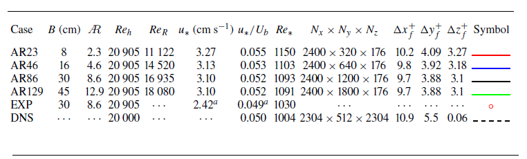
 u∗
 Ub
 Reh=Ubh/ν
 ReR=UbRh/ν
 Re∗=u∗h/ν
 Nx,Ny,Nz
 Δxf+,Δyf+,Δzf+
 a
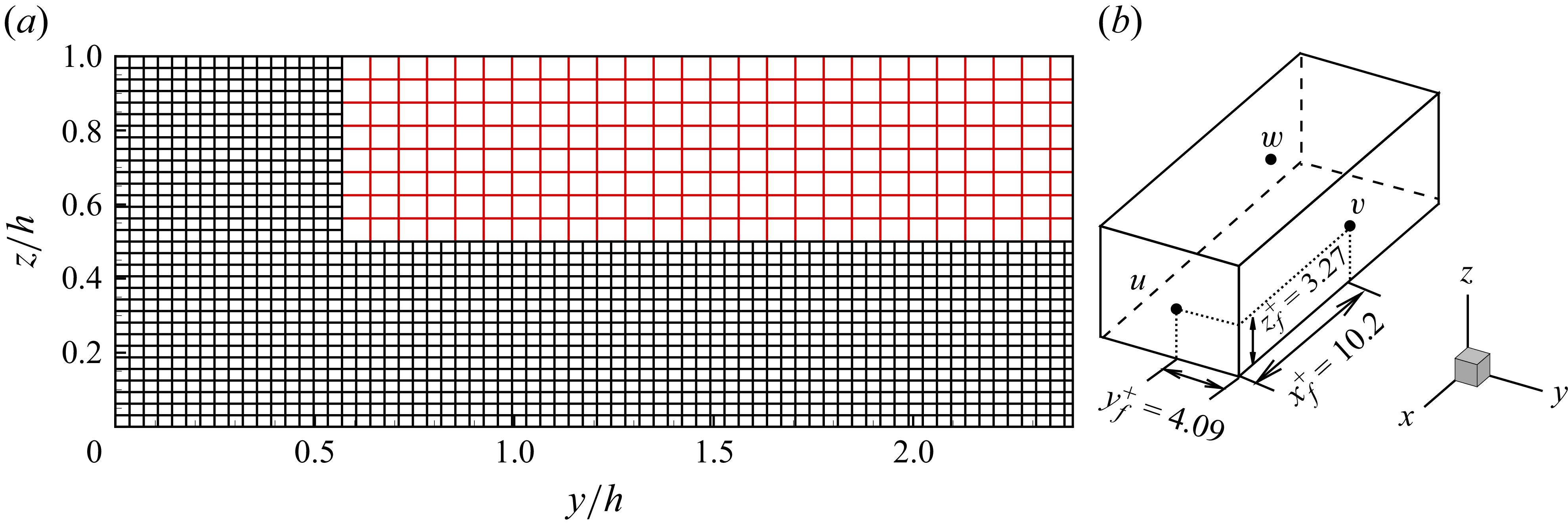
 (a)
 y
 z
 (b)
 Δxf=2.5Δyf≈3.0Δzf
 Δxf+=10.2
 Δyf+=4.09
 Δzf+=3.27
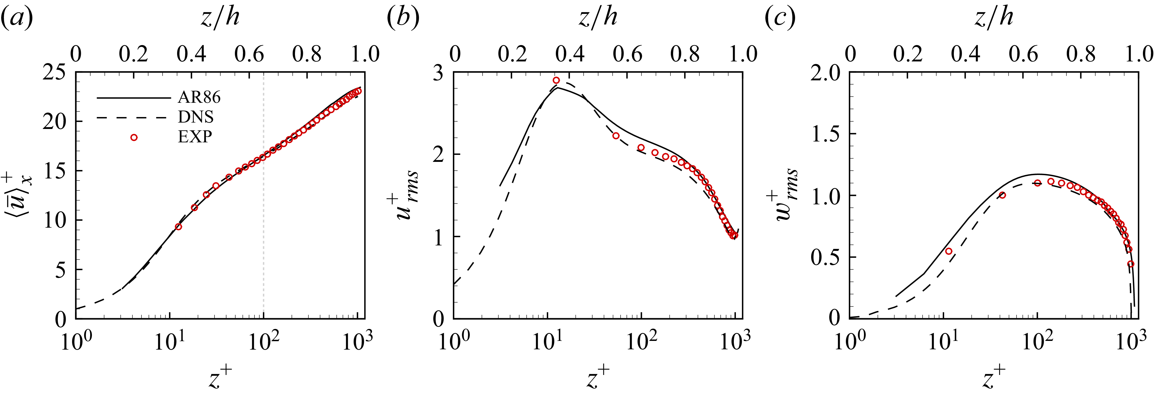
 (a)
 b
 c

 (a)⟨u¯⟩+
 (b)urms+
 (c)vrms+
 (d)wrms+
 (a)
 u+=z+
 u+=(1/κ)ln(z+)+A
 κ=0.39
 A=4.6

 a
 ∂⟨u¯⟩x/∂z
 u∗/h
 b
 −⟨u′w′¯⟩
 u∗2
 c
 ⟨TKEp⟩=−⟨u′w′¯⟩×(∂⟨u¯⟩x/∂z)
 u∗3/h

 ⟨u¯⟩x/Ub
 (a)
 (b)
 (c)
 (d)

 Us/Ub
 (a)
 (b)
 (c)
 (d)

 (a)
 (b)
 (c)
 (d)

 (a)
 (b)
 (c)
 (d)
 u′w′¯=0

 z/h=0.5
 (a)
 (b)
 (c)
 (d)

 a,c,f,j
 y/h=0.5
 b,d,g,k
 y/h=1.0
 e,h,l
 y/h=2.0
 i,m
 y/B=0.5
 kx=2π/λx
 Φuu
 kxΦuu/u∗2<0.1

 a
 z/h=0.2
 b
 z/h=0.5
 c
 z/h=0.75
 d
 z/h=0.9
 0.5
 0.3
 c
 y/h=0.5

 (a,d,g,j)
 z/h=0.2
 (b,e,h,k)
 z/h=0.5
 (c,f,i,l)
 z/h=0.8
 y/h=3.0
 z/h
 kxΦuu/u∗2
 kxΦuu/u∗2
 0.7
 0.4
 0.2
 z/h=0.2
 z/h=0.5
 z/h=0.8
 kxΦuu/u∗2<0.1

 (a)
 (b)
 (c)
 (d)
 0.6
 0.1
 λx=3h
 λx=6h
 λx/h=10
 λx/h=20

 (a)
 (b)
 (a)
 (c)
 (d)
 λx/h=6
 a
 λx/h=20
 b

 v˙/Ub,w˙/Ub
 (a−f)
 (g−l)
 (a)
 (d)
 (a)

 v˙/Ub,w˙/Ub
 (a−f)
 (g−l)
 (a)
 (d)
 (a)

 v˙/Ub,w˙/Ub
 (a−f)
 (g−l)
 (a)
 (d)
 (a)

 Ruu
 a,b
 c,d
 a,c
 z/h=0.2
 y/h=0.5
 b,d
 z/h=0.2
 y/B=0.5
 Ruu=0.1
 Ruu=−0.1

 (a,b)
 (c,d)
 (a,c)
 (b,d)
 0.6

 kxΦuu/u∗2
 (a
 d)
 Lx≈42h
 (e
 h)
 Lx=80h
 (a,e)
 y/h=0.5
 (b,f)
 y/h=1.0
 (c,g)
 y/h=2.0
 (d,h)
 y/B=0.5

 Us/Ub
 (a)
 (b)

 kxΦuu/urms2(z)
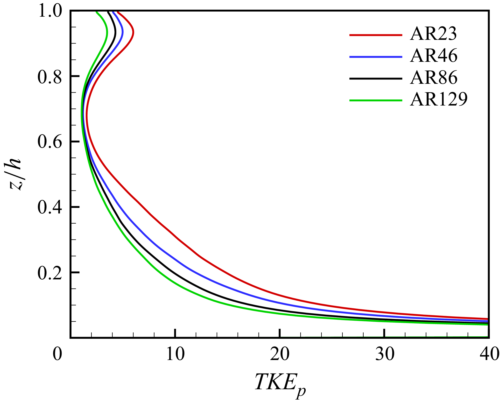
 TKEp∗h/u∗3
 y/h=0.5
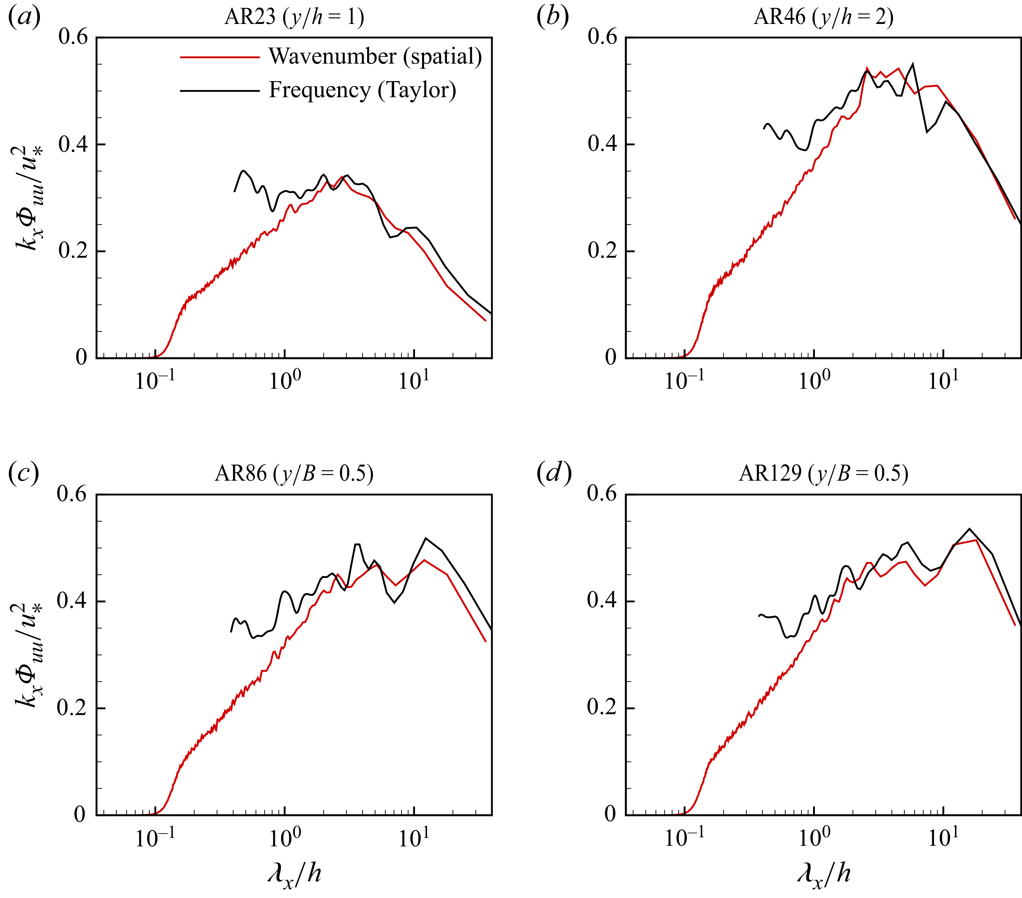
 kxΦuu/u∗2
 z/h=0.5
 (a)
 (b)
 (c)
 (d)

 Open access

