1. Introduction
Magnetic reconnection consists of a modification of the topology of a magnetic field in a plasma and is one of the most promising candidates to explain the rapid thermal and kinetic energy releases occurring in phenomena such as solar flares, magnetic substorms and sawtooth oscillations in tokamaks (Biskamp Reference Biskamp2000; Priest & Forbes Reference Priest and Forbes2000; Yamada, Kulsrud & Ji Reference Yamada, Kulsrud and Ji2010). In weakly collisional plasmas, such as those present in the magnetosphere and in tokamak cores, magnetic reconnection can often be triggered by non-dissipative mechanisms. In particular, in such plasmas, finite electron inertia can provide an effective non-dissipative mechanism to break the magnetic frozen-in condition and therefore allow for magnetic reconnection to take place (Coppi Reference Coppi1964).
A considerable effort has been devoted to the modelling of magnetic reconnection mediated by electron inertia (often referred to as ‘inertial reconnection’) by means of fluid models. The literature on the subject is vast and we indicate Biskamp (Reference Biskamp2000) and Yamada et al. (Reference Yamada, Kulsrud and Ji2010) as well as the works cited therein, for the description of applications and limitations of such models. Given its non-dissipative nature, models aiming at describing inertial reconnection are supposed to have Hamiltonian character. This has naturally motivated an effort, originated with Schep, Pegoraro & Kuvshinov (Reference Schep, Pegoraro and Kuvshinov1994), for deriving Hamiltonian fluid models for inertial reconnection in slab geometry, in particular in the presence of a strong magnetic guide field. The knowledge of the Hamiltonian structure, in addition to providing an unambiguous expression for the total conserved energy for the system, has offered means to gain further insights on the reconnection dynamics. For instance, the existence of alternative topological constraints on the reconnection process has been unveiled, thanks to the knowledge of the Casimir invariants associated with the Hamiltonian structure (Cafaro et al. Reference Cafaro, Grasso, Pegoraro, Porcelli and Saluzzi1998). The presence of such invariants also helped in understanding the formation of small-scale structures in vorticity and current density fields in the nonlinear phase of the reconnection process (Grasso et al. Reference Grasso, Califano, Pegoraro and Porcelli2001). The role of such invariants in inhibiting secondary fluid instabilities has been discussed in Del Sarto, Califano & Pegoraro (Reference Del Sarto, Califano and Pegoraro2006) and Grasso et al. (Reference Grasso, Borgogno, Pegoraro and Tassi2009). Stability conditions and the presence of negative-energy modes for equilibria of inertial reconnection fluid models (Kuvshinov, Pegoraro & Schep Reference Kuvshinov, Pegoraro and Schep1994; Tassi et al. Reference Tassi, Morrison, Waelbroeck and Grasso2008) have also been derived, making use of the energy-Casimir method, which is based on the non-canonical Poisson brackets of the models (see e.g. Holm et al. Reference Holm, Marsden, Ratiu and Weinstein1985; Morrison Reference Morrison1998).
To the best of our knowledge, all fluid models, with a known Hamiltonian structure, adopted so far to investigate inertial reconnection, evolve at most two fluid moments for each particle species and assume simple closure relations, of either isothermal or adiabatic type, for the pressure perturbations in the direction along the magnetic guide field. A natural question concerns then the derivation of more refined Hamiltonian fluid models for inertial reconnection that could describe the evolution of higher-order moments, such as heat fluxes. In particular, for weakly collisional low-
 ${\it\beta}$
plasmas (where we indicate with
 ${\it\beta}$
the ratio between thermal and magnetic pressures, the latter based on the guide field), the limitations of isothermal closures for the electron fluid have been pointed out (de Blank Reference de Blank2001; Zocco & Schekochihin Reference Zocco and Schekochihin2011).
The purpose of the present paper is two-fold. First, we present a Hamiltonian six-field fluid model for inertial reconnection, coupling the evolution of an isothermal ion fluid, retaining finite Larmor radius effects, with that of an electron fluid characterized by a non-isothermal closure accounting for parallel temperature and heat flux evolutions. In the second place, we intend to make use of this model, and of its Hamiltonian structure, to investigate some characteristic features of inertial reconnection such as linear growth rates, widths of the macroscopic magnetic island and energy redistribution. We also intend to compare the results obtained from the six-field model with those obtained from a previous Hamiltonian four-field model with isothermal electrons (Waelbroeck & Tassi Reference Waelbroeck and Tassi2012). This could provide information on the role played by temperature and heat fluxes in inertial reconnection in the framework of a Hamiltonian fluid description. The present investigation aims then at progressing in the description of inertial reconnection in the framework of Hamiltonian fluid models. Clearly, the role of higher-order moments in collisionless reconnection has also been investigated with alternative approaches. For instance, investigations by means of a kinetic model have proved the relevance of electron heat flux contributions to the electric field in a region with the size of the order of the electron Larmor radius surrounding the null point (Hesse, Kuznetsova & Birn Reference Hesse, Kuznetsova and Birn2004). Also, a hybrid fluid/kinetic model has been adopted to analyse the transfer of energy to higher-order moments and the role of dissipation, in inertial reconnection, due to electron Landau damping (Loureiro, Schekochihin & Zocco Reference Loureiro, Schekochihin and Zocco2013).
The paper is organized as follows. In § 2 the six-field model is introduced and in § 3 its Hamiltonian structure is presented and discussed. Section 4 presents a comparison between the six-field model and the isothermal four-field model. In § 5 the role of the sound Larmor radius parameter on the dynamics of temperature and heat flux is investigated numerically, whereas § 6 describes a qualitative reinterpretation of the field structures in terms of Lagrangian invariants. We conclude in § 7.
2. Model equations
In a Cartesian coordinate system
 $(x,y,z)$
the model consists of the evolution equations
 $$\begin{eqnarray}\displaystyle & \displaystyle \frac{\partial n_{e}}{\partial t}+[{\it\phi},n_{e}]-[A,u_{e}]=0, & \displaystyle\end{eqnarray}$$
 $$\begin{eqnarray}\displaystyle & \displaystyle \frac{\partial F}{\partial t}+[{\it\phi},F]+{\it\rho}_{s}^{2}[A,T_{\Vert }+n_{e}]=0, & \displaystyle\end{eqnarray}$$
 $$\begin{eqnarray}\displaystyle & \displaystyle \frac{\partial T_{\Vert }}{\partial t}+[{\it\phi},T_{\Vert }]-2[A,q_{\Vert }+u_{e}]=0, & \displaystyle\end{eqnarray}$$
 $$\begin{eqnarray}\displaystyle & \displaystyle \frac{\partial q_{\Vert }}{\partial t}+[{\it\phi},q_{\Vert }]-\frac{3}{2}\frac{{\it\rho}_{s}^{2}}{d_{e}^{2}}[A,T_{\Vert }]=0, & \displaystyle\end{eqnarray}$$
 $$\begin{eqnarray}\displaystyle & \displaystyle \frac{\partial n_{i}}{\partial t}+[{\it\Phi},n_{i}]+[u_{i},\mathscr{A}]=0, & \displaystyle\end{eqnarray}$$
 $$\begin{eqnarray}\displaystyle & \displaystyle \frac{\partial D}{\partial t}+[{\it\Phi},D]+{\it\rho}_{i}^{2}[n_{i},\mathscr{A}]=0, & \displaystyle\end{eqnarray}$$
 $$\begin{eqnarray}\frac{{\it\Gamma}_{0}-1}{{\it\rho}_{i}^{2}}{\it\phi}+{\it\Gamma}_{0}^{1/2}n_{i}-n_{e}=0\end{eqnarray}$$
and by Ampère’s law
 $$\begin{eqnarray}{\rm\nabla}^{2}A+{\it\Gamma}_{0}^{1/2}u_{i}-u_{e}=0.\end{eqnarray}$$
In (2.1)–(2.6),
 $n_{i,e}$
are the guiding centre and electron density fluctuations with respect to a constant uniform density background
 $n_{0}$
,
 ${\it\phi}$
is the electrostatic potential and
 $A$
is the magnetic flux function. The expression of the corresponding magnetic field is given by
 $\boldsymbol{B}=\boldsymbol{{\rm\nabla}}A\times \hat{z}+B\hat{z}$
, with
 $B$
indicating the amplitude of the constant and uniform guide field. The fields
 $F$
and
 $D$
are defined as
 $F=A-d_{e}^{2}u_{e}$
and
 $D=\mathscr{A}+d_{i}^{2}u_{i}$
, with
 $d_{i,e}$
and
 $u_{i,e}$
indicating the ion and electron skin depths and fluid velocities along the guide field, respectively. The gyroaveraged magnetic flux function and electrostatic potential are defined as
 $\mathscr{A}={\it\Gamma}_{0}^{1/2}A$
and
 ${\it\Phi}={\it\Gamma}_{0}^{1/2}{\it\phi}$
, where the operator
 ${\it\Gamma}_{0}$
corresponds, in Fourier space, to the multiplication times
 $\text{I}_{0}(k_{\bot }^{2}{\it\rho}_{i}^{2})\exp (-k_{\bot }^{2}{\it\rho}_{i}^{2})$
, with
 $\text{I}_{0}$
indicating the modified Bessel function of order zero and
 $k_{\bot }^{2}=k_{x}^{2}+k_{y}^{2}$
indicating the squared wavenumber in the
 $xy$
plane. The constants
 ${\it\rho}_{i,s}$
represent the thermal ion Larmor radius and the sonic Larmor radius, respectively. The fields
 $T_{\Vert }$
and
 $q_{\Vert }$
, on the other hand, indicate the fluctuations of the electron parallel temperature and heat flux, respectively. Finally, the bracket
 $[\,,]$
is defined as
 $[f,g]=\partial _{x}f\partial _{y}g-\partial _{y}f\partial _{x}g$
, for two functions
 $f$
and
 $g$
.
The above-defined quantities are dimensionless and their relation with dimensional quantities is the following:
 $$\begin{eqnarray}\left.\begin{array}{@{}c@{}}\displaystyle t=\frac{v_{A}}{L}\hat{t},\quad x=\frac{\hat{x}}{L},\quad d_{i,e}=\frac{\hat{d}_{i,e}}{L},\quad {\it\rho}_{i,s}=\frac{\hat{{\it\rho}}_{i,s}}{L},\\ \displaystyle n_{i,e}=\frac{L}{\hat{d}_{i}}\frac{\hat{n}_{i,e}}{n_{0}},\quad u_{i,e}=\frac{L}{\hat{d}_{i}}\frac{\hat{u} _{i,e}}{v_{A}},\quad A=\frac{\hat{A_{\Vert }}}{BL},\quad {\it\phi}=\frac{\hat{{\it\phi}}}{BLv_{A}},\\ \displaystyle T_{\Vert }=\frac{L}{\hat{d}_{i}}\frac{\hat{T}_{\Vert }}{T_{0}},\quad q_{\Vert }=\frac{L}{\hat{d}_{i}}\frac{\hat{q}_{\Vert }}{n_{0}v_{A}T_{0}},\end{array}\right\}\end{eqnarray}$$
with
 $L$
,
 $n_{0}$
,
 $T_{0}$
and
 $v_{A}$
representing a characteristic scale length, the equilibrium uniform density and electron temperature and the Alfvén speed based on
 $B$
, respectively. In (2.9), we indicated with carets the dimensional quantities.
The fields
 $n_{i},n_{e},F,D,T_{\Vert }$
and
 $q_{\Vert }$
are supposed to possess translational invariance along the
 $z$
coordinate, although the extension to a three-dimensional model, under the assumption of a strong guide field, is straightforward.
The six-field model (2.1)–(2.8) represents an extension of the four-field gyrofluid model derived and investigated in Comisso et al. (Reference Comisso, Grasso, Tassi and Waelbroeck2012) and Waelbroeck & Tassi (Reference Waelbroeck and Tassi2012). Indeed, the four-field model assumed an isothermal closure for the electron fluid, whereas the six-field model allows for an evolution of the parallel electron temperature and heat flux. On the other hand, the six-field model can be seen as a simplified version of the gyrofluid models of Snyder & Hammett (Reference Snyder and Hammett2001) and Scott (Reference Scott2010) when parallel dynamics, background inhomogeneities, dissipation and moments involving the perpendicular velocities are neglected. Also, our six-field model assumes an isothermal ion fluid and standard closures for the gyroaveraging operators. Electron inertia, which provides the mechanism for magnetic reconnection, is retained, as in Scott (Reference Scott2010), but unlike Snyder & Hammett (Reference Snyder and Hammett2001). Upon denoting with
 ${\it\beta}_{e}$
the
 ${\it\beta}$
parameter referred to the electron pressure, and with
 $m_{i}$
and
 $m_{e}$
the ion and electron masses, respectively, we can recall the relation
 ${\it\rho}_{s}^{2}/d_{e}^{2}=(1/2){\it\beta}_{e}(m_{i}/m_{e})$
. Therefore, as a consequence of retaining finite electron inertia, the ratio between
 ${\it\rho}_{s}$
and
 $d_{e}$
corresponds to determining the
 ${\it\beta}_{e}$
parameter.
3. Hamiltonian structure of the model
In this section we show that the six-field model admits a Hamiltonian formulation. This amounts to showing that the evolution equations (2.1)–(2.6), taking into account also (2.7) and (2.8), can be cast in the form
 $$\begin{eqnarray}\frac{\partial {\it\chi}_{i}}{\partial t}=\{{\it\chi}_{i},H\},\quad i=1,\dots ,6,\end{eqnarray}$$
where the fields
 $\{{\it\chi}_{i}\}_{i=1,\dots ,6}$
are six appropriate dynamical variables,
 $H$
is the Hamiltonian functional and
 $\{\,,\}$
is a Poisson bracket.
Given the formulation of the model (2.1)–(2.6), a natural choice for the six dynamical variables corresponds to
 ${\it\chi}_{1}=n_{e}$
,
 ${\it\chi}_{2}=F$
,
 ${\it\chi}_{3}=T_{\Vert }$
,
 ${\it\chi}_{4}=q_{\Vert }$
,
 ${\it\chi}_{5}=n_{i}$
and
 ${\it\chi}_{6}=D$
.
With regard to the Hamiltonian, a good candidate is provided by the functional
 $$\begin{eqnarray}H=\frac{1}{2}\int \text{d}^{2}x\left({\it\rho}_{i}^{2}n_{i}^{2}+{\it\rho}_{s}^{2}n_{e}^{2}+d_{i}^{2}u_{i}^{2}+d_{e}^{2}u_{e}^{2}-A{\rm\nabla}^{2}A+{\it\Phi}n_{i}-{\it\phi}n_{e}+\frac{{\it\rho}_{s}^{2}}{2}T_{\Vert }^{2}+\frac{2}{3}d_{e}^{2}q_{\Vert }^{2}\right).\end{eqnarray}$$
This quantity has indeed been shown to be conserved by the model equations (Scott Reference Scott2010), which is a necessary condition for it to be the Hamiltonian of the system. We also remark that the functional equation (3.2) can be seen as the sum of the Hamiltonian of the four-field model of Comisso et al. (Reference Comisso, Grasso, Tassi and Waelbroeck2012), corresponding to the first seven terms accounting for kinetic, internal and electromagnetic energy, with the internal energy associated with temperature and heat flux fluctuations, provided by the last two terms.
Concerning the Poisson bracket, the structure of the model equations suggests that it be of the form
 $$\begin{eqnarray}\{\mathscr{F},\mathscr{G}\}=\mathop{\sum }_{i,j,k=1}^{6}\unicode[STIX]{x1D652}_{k}^{ij}\int \text{d}^{2}x{\it\chi}_{k}[\mathscr{F}_{{\it\chi}_{i}},\mathscr{G}_{{\it\chi}_{j}}],\end{eqnarray}$$
where
 $\unicode[STIX]{x1D652}_{k}^{ij}$
are constant coefficients and subscripts on functionals indicate functional derivatives, so that
 $\mathscr{F}_{{\it\chi}_{i}}={\it\delta}\mathscr{F}/{\it\delta}{\it\chi}_{i}$
. We recall that a Poisson bracket is an operation that has to satisfy bilinearity, the Leibniz identity, antisymmetry and the Jacobi identity. The first two of these properties are automatically satisfied by a bracket of the form (3.3). Antisymmetry and the Jacobi identity, on the other hand, impose constraints on the coefficients
 $\unicode[STIX]{x1D652}_{k}^{ij}$
. In particular, as shown in Thiffeault & Morrison (Reference Thiffeault and Morrison2000), for antisymmetry to be satisfied the coefficients must be symmetric in their upper indices, that is,
 $$\begin{eqnarray}\unicode[STIX]{x1D652}_{k}^{ij}=\unicode[STIX]{x1D652}_{k}^{ji}.\end{eqnarray}$$
The Jacobi identity, on the other hand, is satisfied if and only if the matrices
 $\unicode[STIX]{x1D652}^{(j)}$
pairwise commute. These matrices are defined as
 $$\begin{eqnarray}[\unicode[STIX]{x1D652}^{(j)}]_{k}^{i}=\unicode[STIX]{x1D652}_{k}^{ij},\quad j=1,\dots ,6,\end{eqnarray}$$
with
 $k$
labelling rows and
 $i$
labelling columns. Relying on this result, we can proceed to construct the Poisson bracket following the same procedure adopted in the case of other reduced plasma models (see e.g. Hazeltine, Hsu & Morrison Reference Hazeltine, Hsu and Morrison1987; Waelbroeck, Morrison & Horton Reference Waelbroeck, Morrison and Horton2004; Tassi et al.
Reference Tassi, Morrison, Waelbroeck and Grasso2008). More precisely, we can look for a set of six matrices
 $\unicode[STIX]{x1D652}^{(j)}$
satisfying (3.4) and (3.5) and such that the corresponding equations of motion
 $$\begin{eqnarray}\frac{\partial {\it\chi}_{i}}{\partial t}=\mathop{\sum }_{j,k=1}^{6}\unicode[STIX]{x1D652}_{k}^{ij}[H_{{\it\chi}_{j}},{\it\chi}_{k}],\quad i=1,\dots ,6,\end{eqnarray}$$
obtained using (3.1)–(3.3), match the evolution equations (2.1)–(2.6).
With the help of the relations
 $$\begin{eqnarray}H_{n_{e}}={\it\rho}_{s}^{2}n_{e}-{\it\phi},\quad H_{F}=-u_{e},\quad H_{T_{\Vert }}=\frac{{\it\rho}_{s}^{2}}{2}T_{\Vert },\end{eqnarray}$$
 $$\begin{eqnarray}H_{q_{\Vert }}={\textstyle \frac{2}{3}}d_{e}^{2}q_{\Vert },\quad H_{n_{i}}={\it\rho}_{i}^{2}n_{i}+{\it\Phi},\quad H_{D}=u_{i},\end{eqnarray}$$
one finds that the set of pairwise commuting matrices
 $\unicode[STIX]{x1D652}^{(j)}$
yielding a Poisson bracket as well as the desired equations of motion can be written as
 $$\begin{eqnarray}\left.\begin{array}{@{}c@{}}\unicode[STIX]{x1D652}^{(1)}=\left(\begin{array}{@{}cccccc@{}}1 & 0 & 0 & 0 & 0 & 0\\ 0 & 1 & 0 & 0 & 0 & 0\\ 0 & 0 & 1 & 0 & 0 & 0\\ 0 & 0 & 0 & 1 & 0 & 0\\ 0 & 0 & 0 & 0 & 0 & 0\\ 0 & 0 & 0 & 0 & 0 & 0\end{array}\right),\quad \unicode[STIX]{x1D652}^{(2)}=\left(\begin{array}{@{}cccccc@{}}0 & {\it\rho}_{s}^{2}d_{e}^{2} & 0 & 0 & 0 & 0\\ 1 & 0 & 2 & 0 & 0 & 0\\ 0 & {\it\rho}_{s}^{2}d_{e}^{2} & 0 & -3{\it\rho}_{s}^{2}/2 & 0 & 0\\ 0 & 0 & -2d_{e}^{2} & 0 & 0 & 0\\ 0 & 0 & 0 & 0 & 0 & 0\\ 0 & 0 & 0 & 0 & 0 & 0\end{array}\right),\\ \unicode[STIX]{x1D652}^{(3)}=\left(\begin{array}{@{}cccccc@{}}0 & 0 & 2 & 0 & 0 & 0\\ 0 & 2 & 0 & -3/d_{e}^{2} & 0 & 0\\ 1 & 0 & 4 & 0 & 0 & 0\\ 0 & -2d_{e}^{2} & 0 & 2 & 0 & 0\\ 0 & 0 & 0 & 0 & 0 & 0\\ 0 & 0 & 0 & 0 & 0 & 0\end{array}\right),\quad \unicode[STIX]{x1D652}^{(4)}=\left(\begin{array}{@{}cccccc@{}}0 & 0 & 0 & 3{\it\rho}_{s}^{2}/(2d_{e}^{2}) & 0 & 0\\ 0 & 0 & -3/d_{e}^{2} & 0 & 0 & 0\\ 0 & -3{\it\rho}_{s}^{2}/2 & 0 & 3{\it\rho}_{s}^{2}/(2d_{e}^{2}) & 0 & 0\\ 1 & 0 & 2 & 0 & 0 & 0\\ 0 & 0 & 0 & 0 & 0 & 0\\ 0 & 0 & 0 & 0 & 0 & 0\end{array}\right),\\ \unicode[STIX]{x1D652}^{(5)}=\left(\begin{array}{@{}cccccc@{}}0 & 0 & 0 & 0 & 0 & 0\\ 0 & 0 & 0 & 0 & 0 & 0\\ 0 & 0 & 0 & 0 & 0 & 0\\ 0 & 0 & 0 & 0 & 0 & 0\\ 0 & 0 & 0 & 0 & -1 & 0\\ 0 & 0 & 0 & 0 & 0 & -1\end{array}\right),\quad \unicode[STIX]{x1D652}^{(6)}=\left(\begin{array}{@{}cccccc@{}}0 & 0 & 0 & 0 & 0 & 0\\ 0 & 0 & 0 & 0 & 0 & 0\\ 0 & 0 & 0 & 0 & 0 & 0\\ 0 & 0 & 0 & 0 & 0 & 0\\ 0 & 0 & 0 & 0 & 0 & -{\it\rho}_{i}^{2}d_{i}^{2}\\ 0 & 0 & 0 & 0 & -1 & 0\end{array}\right).\end{array}\right\}\end{eqnarray}$$
From (3.3) and (3.9), it follows then that the Poisson bracket for the model (2.1)–(2.6) is given by
 $$\begin{eqnarray}\{\mathscr{F},\mathscr{G}\}=\{\mathscr{F},\mathscr{G}\}_{e}+\{\mathscr{F},\mathscr{G}\}_{i},\end{eqnarray}$$
where
 $$\begin{eqnarray}\displaystyle \{\mathscr{F},\mathscr{G}\}_{e} & = & \displaystyle \int \text{d}^{2}x\left[n_{e}\left([\mathscr{F}_{n_{e}},\mathscr{G}_{n_{e}}]+{\it\rho}_{s}^{2}d_{e}^{2}[\mathscr{F}_{F},\mathscr{G}_{F}]+2[\mathscr{F}_{T_{\Vert }},\mathscr{G}_{T_{\Vert }}]+\frac{3}{2}\frac{{\it\rho}_{s}^{2}}{d_{e}^{2}}[\mathscr{F}_{q_{\Vert }},\mathscr{G}_{q_{\Vert }}]\right)\right.\nonumber\\ \displaystyle & & \displaystyle +\,F\left(\vphantom{\frac{3}{2}}[\mathscr{F}_{F},\mathscr{G}_{n_{e}}]+[\mathscr{F}_{n_{e}},\mathscr{G}_{F}]+2([\mathscr{F}_{F},\mathscr{G}_{T_{\Vert }}]+[\mathscr{F}_{T_{\Vert }},\mathscr{G}_{F}])\right.\nonumber\\ \displaystyle & & \displaystyle -\,\left.\frac{3}{d_{e}^{2}}([\mathscr{F}_{q_{\Vert }},\mathscr{G}_{T_{\Vert }}]+[\mathscr{F}_{T_{\Vert }},\mathscr{G}_{q_{\Vert }}])\right)\nonumber\\ \displaystyle & & \displaystyle +\,T_{\Vert }\left([\mathscr{F}_{T_{\Vert }},\mathscr{G}_{n_{e}}]+[\mathscr{F}_{n_{e}},\mathscr{G}_{T_{\Vert }}]+{\it\rho}_{s}^{2}d_{e}^{2}[\mathscr{F}_{F},\mathscr{G}_{F}]\vphantom{\frac{3}{2}}\right.\nonumber\\ \displaystyle & & \displaystyle \left.-\,\frac{3}{2}{\it\rho}_{s}^{2}([\mathscr{F}_{q_{\Vert }},\mathscr{G}_{F}]+[\mathscr{F}_{F},\mathscr{G}_{q_{\Vert }}])+4[\mathscr{F}_{T_{\Vert }},\mathscr{G}_{T_{\Vert }}]+\frac{3}{2}\frac{{\it\rho}_{s}^{2}}{d_{e}^{2}}[\mathscr{F}_{q_{\Vert }},\mathscr{G}_{q_{\Vert }}]\right)\nonumber\\ \displaystyle & & \displaystyle +\,q_{\Vert }\left([\mathscr{F}_{q_{\Vert }},\mathscr{G}_{n_{e}}]+[\mathscr{F}_{n_{e}},\mathscr{G}_{q_{\Vert }}]-2d_{e}^{2}([\mathscr{F}_{T_{\Vert }},\mathscr{G}_{F}]+[\mathscr{F}_{F},\mathscr{G}_{T_{\Vert }}])\right.\nonumber\\ \displaystyle & & \displaystyle +\,2\left.\vphantom{\frac{3}{2}}\left.([\mathscr{F}_{q_{\Vert }},\mathscr{G}_{T_{\Vert }}]+[\mathscr{F}_{T_{\Vert }},\mathscr{G}_{q_{\Vert }}])\right)\right],\end{eqnarray}$$
 $$\begin{eqnarray}\displaystyle \{\mathscr{F},\mathscr{G}\}_{i} & = & \displaystyle -\int \text{d}^{2}x\left(n_{i}\left([\mathscr{F}_{n_{i}},\mathscr{G}_{n_{i}}]+{\it\rho}_{i}^{2}d_{i}^{2}[\mathscr{F}_{D},\mathscr{G}_{D}]\right)+D\left([\mathscr{F}_{D},\mathscr{G}_{n_{i}}]+[\mathscr{F}_{n_{i}},\mathscr{G}_{D}]\right)\right).\nonumber\\ \displaystyle & & \displaystyle\end{eqnarray}$$
 $\{\,,\,\}_{e}$
and
 $\{\,,\,\}_{i}$
are Poisson brackets of their own and that the corresponding Hamiltonian operators are functions of independent sets of variables. These two brackets evolve independently the electron and ion fluid variables, the coupling between which is provided by the Hamiltonian (3.2). In particular, the bracket
 $\{\,,\,\}_{i}$
is already present in the direct sum for the Poisson bracket of the isothermal model (Waelbroeck & Tassi Reference Waelbroeck and Tassi2012).
Solutions
 $\mathscr{C}$
of the equation
 $$\begin{eqnarray}\{\mathscr{C},\mathscr{F}\}=0,\end{eqnarray}$$
valid for any functional
 $\mathscr{F}$
of the dynamical variables, are Casimir invariants of the system. These functionals foliate the phase space and are preserved by the dynamics (see e.g. Morrison Reference Morrison1998). For the Poisson bracket (3.10), they correspond to the following six infinite families of functionals:
 $$\begin{eqnarray}\displaystyle & \displaystyle C_{i}=\int \text{d}^{2}x\,\mathscr{C}_{i}(G_{i}),\quad i=1,\dots ,4, & \displaystyle\end{eqnarray}$$
 $$\begin{eqnarray}\displaystyle & \displaystyle C_{\pm }=\int \text{d}^{2}x\,\mathscr{C}_{\pm }(I_{\pm }), & \displaystyle\end{eqnarray}$$
 $$\begin{eqnarray}\displaystyle & \displaystyle G_{1}=F-\frac{d_{e}{\it\rho}_{s}}{\sqrt{3+\sqrt{6}}}n_{e}-d_{e}{\it\rho}_{s}\sqrt{\frac{1}{2}+\frac{1}{\sqrt{6}}}T_{\Vert }-d_{e}^{2}\sqrt{\frac{2}{3}}q_{\Vert }, & \displaystyle\end{eqnarray}$$
 $$\begin{eqnarray}\displaystyle & \displaystyle G_{2}=F+\frac{d_{e}{\it\rho}_{s}}{\sqrt{3+\sqrt{6}}}n_{e}+d_{e}{\it\rho}_{s}\sqrt{\frac{1}{2}+\frac{1}{\sqrt{6}}}T_{\Vert }-d_{e}^{2}\sqrt{\frac{2}{3}}q_{\Vert }, & \displaystyle\end{eqnarray}$$
 $$\begin{eqnarray}\displaystyle & \displaystyle G_{3}=F+\frac{d_{e}{\it\rho}_{s}}{\sqrt{3-\sqrt{6}}}n_{e}-d_{e}{\it\rho}_{s}\sqrt{\frac{1}{2}-\frac{1}{\sqrt{6}}}T_{\Vert }+d_{e}^{2}\sqrt{\frac{2}{3}}q_{\Vert }, & \displaystyle\end{eqnarray}$$
 $$\begin{eqnarray}\displaystyle & \displaystyle G_{4}=F-\frac{d_{e}{\it\rho}_{s}}{\sqrt{3-\sqrt{6}}}n_{e}+d_{e}{\it\rho}_{s}\sqrt{\frac{1}{2}-\frac{1}{\sqrt{6}}}T_{\Vert }+d_{e}^{2}\sqrt{\frac{2}{3}}q_{\Vert }, & \displaystyle\end{eqnarray}$$
 $$\begin{eqnarray}\displaystyle & \displaystyle I_{\pm }=D\pm d_{i}{\it\rho}_{i}n_{i}, & \displaystyle\end{eqnarray}$$
 $\mathscr{C}_{1,2,3,4}$
and
 $\mathscr{C}_{\pm }$
are arbitrary functions. The Casimirs
 $C_{1,2,3,4}$
and the Casimirs
 $C_{\pm }$
derive from the brackets
 $\{\,,\,\}_{e}$
and
 $\{\,,\,\}_{i}$
, respectively.
The infinite families of Casimirs are associated with Lagrangian invariants of the model. Indeed, if one performs the change of variables
 $(n_{e},F,T_{\Vert },q_{\Vert },n_{i},D)\rightarrow (G_{1},G_{2},G_{3},G_{4},I_{+},I_{-})$
the model equations (2.1)–(2.6) take the remarkable form
 $$\begin{eqnarray}\left.\begin{array}{@{}c@{}}\displaystyle \frac{\partial G_{i}}{\partial t}=-[{\it\phi}_{i},G_{i}],\quad i=1,\dots ,4,\\ \displaystyle \frac{\partial I_{\pm }}{\partial t}=-[{\it\Phi}_{\pm },I_{\pm }],\end{array}\right\}\end{eqnarray}$$
where
 $$\begin{eqnarray}\left.\begin{array}{@{}c@{}}\displaystyle {\it\phi}_{1}={\it\phi}-\sqrt{3+\sqrt{6}}\frac{{\it\rho}_{s}}{d_{e}}A,\quad {\it\phi}_{2}={\it\phi}+\sqrt{3+\sqrt{6}}\frac{{\it\rho}_{s}}{d_{e}}A,\\ {\it\phi}_{3}=\displaystyle {\it\phi}+\sqrt{3-\sqrt{6}}\frac{{\it\rho}_{s}}{d_{e}}A,\quad {\it\phi}_{4}={\it\phi}-\sqrt{3-\sqrt{6}}\frac{{\it\rho}_{s}}{d_{e}}A,\\ \displaystyle {\it\Phi}_{\pm }={\it\Phi}\mp \frac{{\it\rho}_{i}}{d_{i}}\mathscr{A}.\end{array}\right\}\end{eqnarray}$$
The six Lagrangian invariants
 $G_{1},G_{2},G_{3},G_{4},I_{+},I_{-}$
represent ‘normal’ variables (Tassi et al.
Reference Tassi, Morrison, Grasso and Pegoraro2010) for the bracket (3.10).
From (3.21), one then sees that the dynamics of the reconnection model (2.1)–(2.6) actually expresses the advection of six Lagrangian invariants transported by incompressible flows associated with the stream functions (3.22). Such stream functions are reminiscent of those advecting the generalized perturbed distribution functions in the 2D gyrokinetic description from which the model can be derived Scott (Reference Scott2010). Such stream functions are linear combinations of the electrostatic and magnetic potentials, or of their gyroaveraged versions in the case of
 ${\it\Phi}_{\pm }$
. This has its origin at the guiding centre level, where such potentials are associated with the
 $\boldsymbol{E}\times \boldsymbol{B}$
drift and with the free stream of the guiding centres along the poloidal magnetic field.
Lagrangian invariant dynamics underlying collisionless reconnection is a feature observed in earlier Hamiltonian models for reconnection, where isothermal closures were adopted (Cafaro et al. Reference Cafaro, Grasso, Pegoraro, Porcelli and Saluzzi1998; Grasso et al. Reference Grasso, Califano, Pegoraro and Porcelli2000; Waelbroeck, Hazeltine & Morrison Reference Waelbroeck, Hazeltine and Morrison2009; Waelbroeck & Tassi Reference Waelbroeck and Tassi2012). For such models, the connections with drift or gyrokinetic dynamics had been pointed out in de Blank (Reference de Blank2001), Liseikina, Pegoraro & Echkina (Reference Liseikina, Pegoraro and Echkina2004), Pegoraro, Liseikina & Echkina (Reference Pegoraro, Liseikina and Echkina2005a ,Reference Pegoraro, Liseikina and Echkina b ), Comisso et al. (Reference Comisso, Grasso, Tassi and Waelbroeck2012) and Tassi (Reference Tassi2014a ,Reference Tassi b ). The above Hamiltonian structure and the formulation (3.21) of the model show that, when going beyond the isothermal closure and imposing for the electrons a fluid closure consistent with that adopted in Snyder & Hammett (Reference Snyder and Hammett2001) and Scott (Reference Scott2010) in the non-dissipative limit, the model still preserves a Hamiltonian structure and its dynamics still can be entirely interpreted in terms of Lagrangian invariants. We recall that the model (2.1)–(2.6) can be derived from the following gyrokinetic system, written in dimensional form:
 $$\begin{eqnarray}\displaystyle & \displaystyle \frac{\partial g_{i}}{\partial t}+\frac{c}{B}\left[J_{0}\left({\it\phi}-\frac{v}{c}A\right)\!,g_{i}\right]=0, & \displaystyle\end{eqnarray}$$
 $$\begin{eqnarray}\displaystyle & \displaystyle \frac{\partial g_{e}}{\partial t}+\frac{c}{B}\left[{\it\phi}-\frac{v}{c}A,g_{e}\right]=0. & \displaystyle\end{eqnarray}$$
 $$\begin{eqnarray}\frac{e^{2}n_{0}}{T_{i}}({\it\Gamma}_{0}-1){\it\phi}+e\int \text{d}\mathscr{W}(J_{0}g_{i}-g_{e})=0\end{eqnarray}$$
and Ampère’s law
 $$\begin{eqnarray}{\rm\nabla}^{2}A-4{\rm\pi}\frac{e^{2}}{c^{2}}n_{0}\left(\frac{{\it\Gamma}_{0}}{m_{i}}+\frac{1}{m_{e}}\right)A+4{\rm\pi}\frac{e}{c}\int \text{d}\mathscr{W}v(J_{0}g_{i}-g_{e})=0.\end{eqnarray}$$
Equations (3.23) and (3.24) govern the evolution of
 $g_{i}=f_{i}+\mathscr{F}_{i}(e/T_{i})(v/c)J_{0}A$
and
 $g_{e}=f_{e}-\mathscr{F}_{e}(e/T_{0})(v/c)A$
, where
 $e$
is the proton charge,
 $T_{i}$
the ion equilibrium temperature,
 $J_{0}$
the gyroaveraging operator and
 $f_{i,e}(x,y,z,v,{\it\mu},t)$
indicate the perturbations of the ion and electron equilibrium distribution functions
 $\mathscr{F}_{i,e}$
, respectively, which are defined as
 $$\begin{eqnarray}\displaystyle & \displaystyle \mathscr{F}_{i}(v,{\it\mu})=n_{0}\left(\frac{m_{i}}{2{\rm\pi}T_{i}}\right)^{3/2}\text{exp}\left(-\frac{m_{i}v^{2}+2{\it\mu}B}{2T_{i}}\right), & \displaystyle\end{eqnarray}$$
 $$\begin{eqnarray}\displaystyle & \displaystyle \mathscr{F}_{e}(v,{\it\mu})=n_{0}\left(\frac{m_{e}}{2{\rm\pi}T_{0}}\right)^{3/2}\text{exp}\left(-\frac{m_{e}v^{2}+2(m_{e}/m_{i}){\it\mu}B}{2T_{0}}\right). & \displaystyle\end{eqnarray}$$
 $v$
the velocity coordinate along the magnetic guide field direction and with
 ${\it\mu}$
the ion magnetic moment. The volume element
 $\text{d}\mathscr{W}$
is defined as
 $\text{d}\mathscr{W}=2{\rm\pi}B\,\text{d}{\it\mu}\,\text{d}v/m_{i}$
.
The model equations (2.1)–(2.6) can be derived from (3.23) and (3.24) by taking moments with respect to the Hermite polynomials in the parallel velocity coordinate, and truncating the resulting fluid system by imposing that the moment of order four, for the electron fluid, and of order two for the ion fluid, be zero (Scott Reference Scott2010). The quasi-neutrality relation (3.25) and Ampère’s law (3.26) can, on the other hand, be easily identified with (2.7) and (2.8), respectively, upon introducing fluid velocities and densities and applying standard gyroaveraging closure rules (Scott Reference Scott2010).
The parent gyrokinetic system (3.23) and (3.24) also possesses a Hamiltonian structure (Tassi Reference Tassi2014a ), given by the Hamiltonian functional
 $$\begin{eqnarray}H(g_{i},g_{e})=\frac{1}{2}\int \text{d}^{2}x\,\text{d}\mathscr{W}\left[\frac{T_{i}}{\mathscr{F}_{i}}g_{i}^{2}+\frac{T_{0}}{\mathscr{F}_{e}}g_{e}^{2}+e{\it\phi}(J_{0}g_{i}-g_{e})-e\frac{v}{c}A(J_{0}g_{i}-g_{e})\right]\end{eqnarray}$$
and the Poisson bracket
 $$\begin{eqnarray}\{F,G\}=\frac{c}{eB}\int \text{d}^{2}x\,\text{d}\mathscr{W}\,(-g_{i}[F_{g_{i}},G_{g_{i}}]+g_{e}[F_{g_{e}},G_{g_{e}}]).\end{eqnarray}$$
The closure adopted to derive the six-field model preserves then the Hamiltonian character of the parent gyrokinetic model. The Hamiltonian (3.2), in particular, can be derived from the gyrokinetic Hamiltonian (3.28) by replacing
 $g_{i}$
and
 $g_{e}$
with the corresponding truncated expansions in terms of Hermite polynomials. The Casimirs of the gyrokinetic bracket (3.29), on the other hand, are given by
 $$\begin{eqnarray}C_{i}=\int \text{d}^{2}x\,\text{d}\mathscr{W}\,\mathscr{C}_{i}(g_{i}),\quad C_{e}=\int \text{d}^{2}x\,\text{d}\mathscr{W}\,\mathscr{C}_{e}(g_{e}),\end{eqnarray}$$
with
 $\mathscr{C}_{i,e}$
arbitrary functions. Upon applying the fluid closure, such two families of gyrokinetic Casimirs transform into the six families of gyrofluid Casimirs (3.14)–(3.15).
We remark that the model (2.1)–(2.6) can easily be upgraded, following for instance Scott (Reference Scott2010), to an eight-field model accounting also for parallel ion temperature and heat flux fluctuations. The two additional equations would be analogous to (2.3) and (2.4), but with electron quantities replaced by the corresponding ion quantities, and electrostatic and magnetic potentials replaced by their gyroaveraged counterparts. The resulting model would still be Hamiltonian. In the total conserved energy, ion and electron quantities would then enter in the same way. The corresponding Poisson bracket would be the direct sum
 $\{\mathscr{F},\mathscr{G}\}=\{\mathscr{F},\mathscr{G}\}_{e}+\{\mathscr{F},\mathscr{G}\}_{I}$
, where
 $\{\mathscr{F},\mathscr{G}\}_{I}$
is analogous to
 $\{\mathscr{F},\mathscr{G}\}_{e}$
, but with electron quantities replaced by the corresponding ion quantities. Consequently, the eight-field model would possess eight infinite families of Casimirs associated with Lagrangian invariants. Four families of Casimirs analogous to
 $C_{1},\dots ,C_{4}$
, but for the ion species, would indeed be present. Although the extension to the eight-field model appears to be relatively straightforward, for the present numerical investigation we decided to reserve the refined closure for the electron fluid only. Indeed, for the equilibrium state that we consider, which does not include ion density, velocity or temperature gradients, ion fluctuations appear to have little influence on the inertial reconnection dynamics (see for instance Grasso, Tassi & Waelbroeck Reference Grasso, Tassi and Waelbroeck2010 and Comisso et al.
Reference Comisso, Grasso, Tassi and Waelbroeck2012). Actually, most of the magnetic energy turns out to be converted into electron fluctuations, as will also be confirmed in § 4. Consequently, we stick to the six-field model and postpone the inclusion of ion temperature and heat flux effects to future work, where different equilibrium gradients will be considered.
Incidentally, we also remark that the eight-field model could be reduced to another six-field model by neglecting heat fluxes and thus leaving three pairs of equations for densities, parallel canonical momenta and temperatures of ions and electrons, respectively. Such model would also be Hamiltonian. The Hamiltonian functional would be simply obtained from that of the eight-field model by suppressing heat flux terms. The Poisson bracket would, again, be a direct sum of two Poisson brackets, one related to the electron and one to the ion quantities. Such brackets could be obtained from
 $\{\mathscr{F},\mathscr{G}\}_{e}$
and
 $\{\mathscr{F},\mathscr{G}\}_{I}$
by suppressing all the terms depending on heat fluxes and on functional derivatives with respect to them, and by replacing the factor 4 by a factor 1 in the coefficient multiplying
 $T_{\Vert }[\mathscr{F}_{T_{\Vert }},\mathscr{G}_{T_{\Vert }}]$
in
 $\{\mathscr{F},\mathscr{G}\}_{e}$
(and proceeding analogously with
 $\{\mathscr{F},\mathscr{G}\}_{I}$
).
4. Comparison with the isothermal closure
As pointed out in § 2, the six-field model equations reduce to the four-field ones when an isothermal behaviour for the electrons is considered. In this section we intend to highlight the difference between these two sets of equations, by comparing results from simulations obtained for the same set of parameters. We use here an extended version of the pseudo-spectral numerical code adopted in Comisso et al. (Reference Comisso, Grasso, Tassi and Waelbroeck2012), where the fields of the model are decomposed in a time-independent equilibrium and an evolving perturbation which is advanced in time according to a third-order Adams–Bashforth algorithm. In order to investigate the evolution of spontaneous magnetic reconnection instabilities, the system of (2.1)–(2.6) is solved numerically considering an equilibrium which is linearly unstable with respect to tearing modes. In particular, we adopt the following equilibrium:
 $$\begin{eqnarray}{n_{i}}_{eq}(x)={n_{e}}_{eq}(x)=n_{0},\quad {u_{i}}_{eq}(x)=0,\quad A_{eq}(x)=\mathop{\sum }_{n=-11}^{11}\hat{f}_{n}\text{e}^{\text{i}nx},\end{eqnarray}$$
 $$\begin{eqnarray}{T_{\Vert }}_{eq}=0,\quad {q_{\Vert }}_{eq}=0,\end{eqnarray}$$
where we recall that
 $n_{0}$
represents a uniform background density, whereas
 $\hat{f}_{n}$
are the Fourier coefficients of the function
 $$\begin{eqnarray}f(x)=A_{0}/\cosh ^{2}(x),\end{eqnarray}$$
with
 $A_{0}$
representing a parameter that determines the strength of the in-plane equilibrium magnetic field. In the following, we consider
 $A_{0}=0.1$
and restrict ourselves to the strongly unstable regime, which is characterized by large values of the standard instability parameter,
 ${\it\Delta}^{\prime }$
(Furth, Killen & Rosenbluth Reference Furth, Killen and Rosenbluth1963), and which is relevant to the general problem of fast magnetic reconnection. Our integration domain is fixed by
 $L_{x}=2{\rm\pi}$
and
 $L_{y}=4{\rm\pi}$
, while for the physical parameters we choose the following values:
 $d_{e}=0.2$
,
 $d_{i}=2$
,
 ${\it\rho}_{i}=0.2$
and
 ${\it\rho}_{s}=0.01,0.1,0.4$
and 0.8. The first characteristic quantity of the reconnection process that we investigate is the linear growth rate of the perturbation. Figure 1 shows, for different values of
 ${\it\rho}_{s}$
, a comparison of the growth rate, obtained from numerical simulations of the six-field model and of four-field model. The growth rate is measured as the variation of the perturbed magnetic flux at the
 $X$
-point. In the same figure the numerical values are also compared against the analytical predictions obtained by applying the asymptotic formula for the linear growth rate
 ${\it\gamma}_{L}$
given by
 ${\it\gamma}_{L}=0.2k_{y}(2d_{e}{\it\rho}_{{\it\tau}}^{2}/{\rm\pi})^{1/3}$
(Porcelli Reference Porcelli1991; Fitzpatrick & Porcelli Reference Fitzpatrick and Porcelli2004), where
 $k_{y}=2m{\rm\pi}/L_{y}$
,
 $m$
is the mode number and
 ${\it\rho}_{{\it\tau}}=\sqrt{{\it\rho}_{s}^{2}+{\it\rho}_{i}^{2}}$
. This formula is valid for
 ${\it\rho}_{s}^{2}\ll d_{e}^{2}(m_{i}/m_{e})^{3/4}$
and for
 ${\it\Delta}^{\prime }\gg \min [1,(d_{e}/{\it\rho}_{{\it\tau}})^{1/3}]$
. We note that the presence of heat flux fluctuations leads to slightly greater growth rates. The increase in the growth rates is in the range of 5–7 %. On the other hand, the analytic formula overestimates the growth rates, when compared to both the six- and four-field models. The difference is greater for larger values of
 ${\it\rho}_{s}$
, as should be expected when increasing the ratio
 ${\it\rho}_{s}/d_{e}$
at fixed mass ratio. The similarity in the linear growth rates between the six- and four-field models reflects also in similar magnetic island amplitudes at saturation, in agreement with what is observed when a drift-kinetic description is adopted for the electrons (Loureiro et al.
Reference Loureiro, Schekochihin and Zocco2013). We note that this result refers to the large-
 ${\it\Delta}^{\prime }$
regime we are addressing here, and does not extend to small-
 ${\it\Delta}^{\prime }$
regimes, when the island saturation amplitude becomes comparable with the kinetics scales, as already pointed out in Loureiro et al. (Reference Loureiro, Schekochihin and Zocco2013).
Growth rates obtained from the numerical simulations and analytical prediction for different values of
 ${\it\rho}_{s}$
. Asterisks and squares correspond to results of the six- and four-field simulations, respectively, whereas the solid line refers to the analytical prediction.

Subsequently we analyse the energy distribution in the two models. Clearly, the evolution of the heat flux in the six-field model allows the electron temperature to deviate from the isothermal behaviour and opens new energy channels. The different contributions to the total energy are denoted as
 $$\begin{eqnarray}\left.\begin{array}{@{}c@{}}\displaystyle E_{mag}=\frac{1}{2}\int \text{d}^{2}x\,|\boldsymbol{{\rm\nabla}}A|^{2},\quad E_{ke}=\frac{d_{e}^{2}}{2}\int \text{d}^{2}x\,u_{e}^{2},\quad E_{ele}=-\frac{1}{2}\int \text{d}^{2}x\,{\it\phi}n_{e},\\ \displaystyle E_{the}=\frac{{\it\rho}_{s}^{2}}{2}\int \text{d}^{2}x\,n_{e}^{2},\quad E_{T_{\Vert }}=\frac{{\it\rho}_{s}^{2}}{4}\int \text{d}^{2}x\,T_{\Vert }^{2},\quad E_{q_{\Vert }}=\frac{d_{e}^{2}}{3}\int \text{d}^{2}x\,q_{\Vert }^{2},\\ \displaystyle E_{ki}=\frac{d_{i}^{2}}{2}\int \text{d}^{2}x\,u_{i}^{2},\quad E_{eli}=-\frac{1}{2}\int \text{d}^{2}x\,{\it\Phi}n_{i},\quad E_{thi}=\frac{{\it\rho}_{i}^{2}}{2}\int \text{d}^{2}x\,n_{i}^{2}.\end{array}\right\}\end{eqnarray}$$
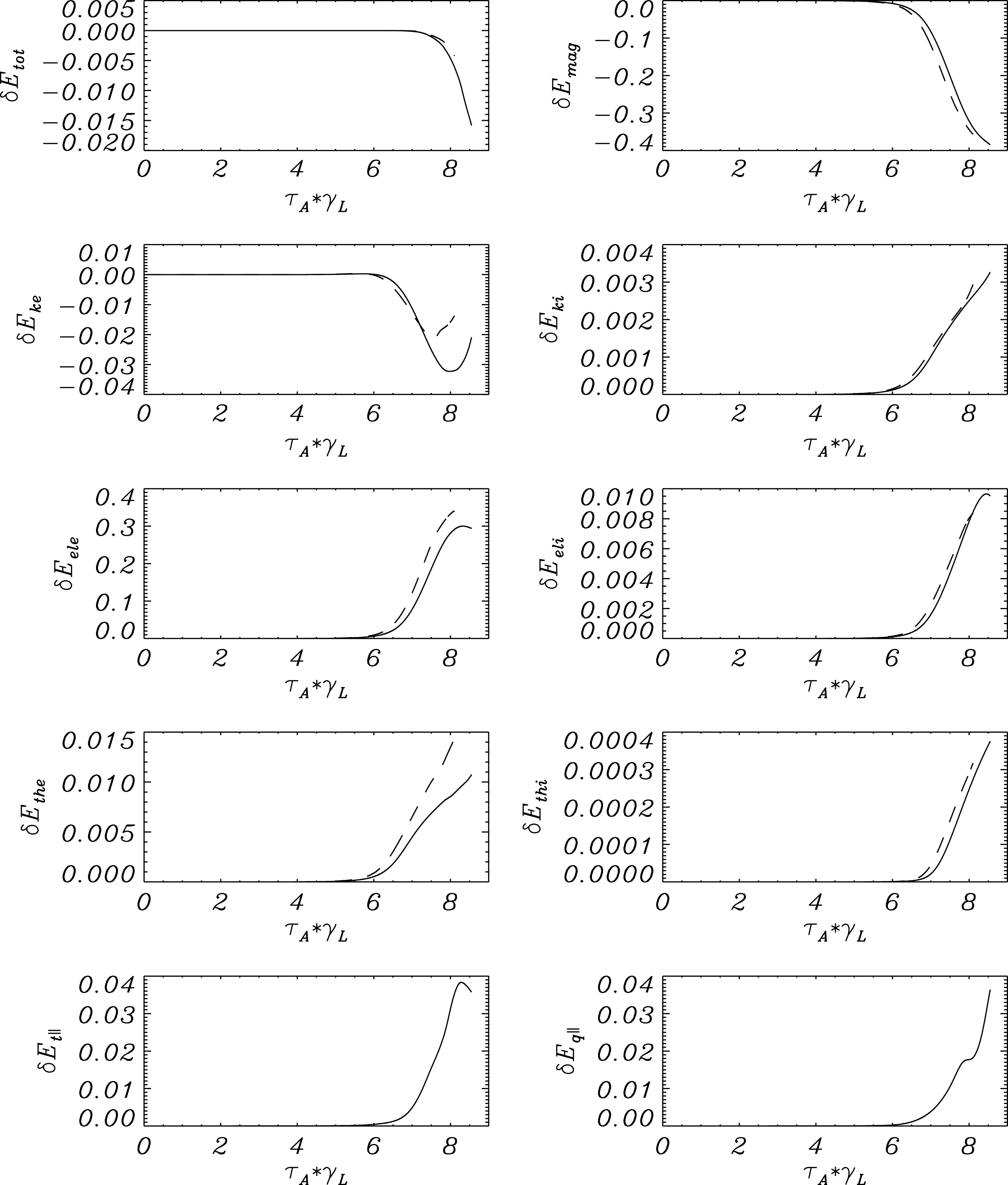
In figure 2, a comparison between the relative variations of the different contributions to the total energy is presented for the case where the ion sound Larmor radius is equal to 0.1. The relative variations for each form of energy are calculated with respect to the initial values and normalized with respect to the total energy, so that, for instance, in the case of the magnetic energy one has
 ${\it\delta}E_{mag}(t)=(E_{mag}(t)-E_{mag}(0))/H(0)$
, where
 $H$
is the Hamiltonian functional (3.2). We compare two simulations that were initialized with the same equilibrium configuration and perturbation and hence the same total energy. The simulations have been stopped when the magnetic island has reached approximately the same macroscopic size. This explains why we find that the behaviour of the converted magnetic energy is similar, as shown in the second panel of figure 2 (we number the panels starting from the left-hand panel in the top row and attributing odd numbers to panels in the left-hand column and even numbers to those in the right-hand column). In both models the magnetic energy,
 $E_{mag}$
, is mainly converted into electron and ion internal energy, shown in the fifth and sixth panels. We remark that the main differences occur in the energies involving the electron quantities, i.e.
 $E_{ke}$
,
 $E_{ele}$
and
 $E_{the}$
shown in the third, fifth and seventh panels, respectively. The smaller amount of magnetic energy converted into these forms in the six-field model is compensated by the energy conversion into internal energy due to the temperature and heat flux fluctuations, that is,
 $E_{T_{\Vert }}$
and
 $E_{q_{\Vert }}$
, shown in the ninth and tenth panels, respectively.
Comparison of relative energy variations between the six-field model (solid lines) and the four-field model (dashed lines) at
 ${\it\rho}_{s}=0.1$
.

5. Dependence on
 ${\it\rho}_{s}$

In this section we examine the dependence of some aspects of the dynamics of the six-field model on the sound Larmor radius
 ${\it\rho}_{s}$
. The motivation for the choice of this parameter is that
 ${\it\rho}_{s}$
is an appropriate variable to investigate the role of heat flux fluctuations, which is the main new ingredient of the six-field model. Indeed, by varying
 ${\it\rho}_{s}$
we can study the transition from a regime with negligible heat flux (
 ${\it\rho}_{s}\ll d_{e}$
), as is the case with an adiabatic equation of state, to a regime with finite heat flux fluctuations. It is worth remembering that
 ${\it\rho}_{s}^{2}/d_{e}^{2}=(1/2){\it\beta}_{e}(M/m_{e})$
. In our simulations we kept fixed both the value of
 $d_{e}=0.2$
and the ratio
 $d_{i}/d_{e}=10$
. Hence, the value of
 ${\it\rho}_{s}$
can also be seen as a measure of the value of the
 ${\it\beta}_{e}$
parameter.
Examining the model equations (2.1)–(2.6), we see that in the limit
 ${\it\rho}_{s}\ll d_{e}$
the heat flux (2.4) tends to decouple from the system. Because we set the initial heat flux equal to zero, we expect it then not to increase significantly. It hence follows, by comparing (2.1) and (2.3), that
 $n_{e}\approx T_{\Vert }/2$
, given that
 $n_{e}(x,y,0)=T_{\Vert }(x,y,0)/2=0$
. On the contrary, when increasing the value of
 ${\it\rho}_{s}$
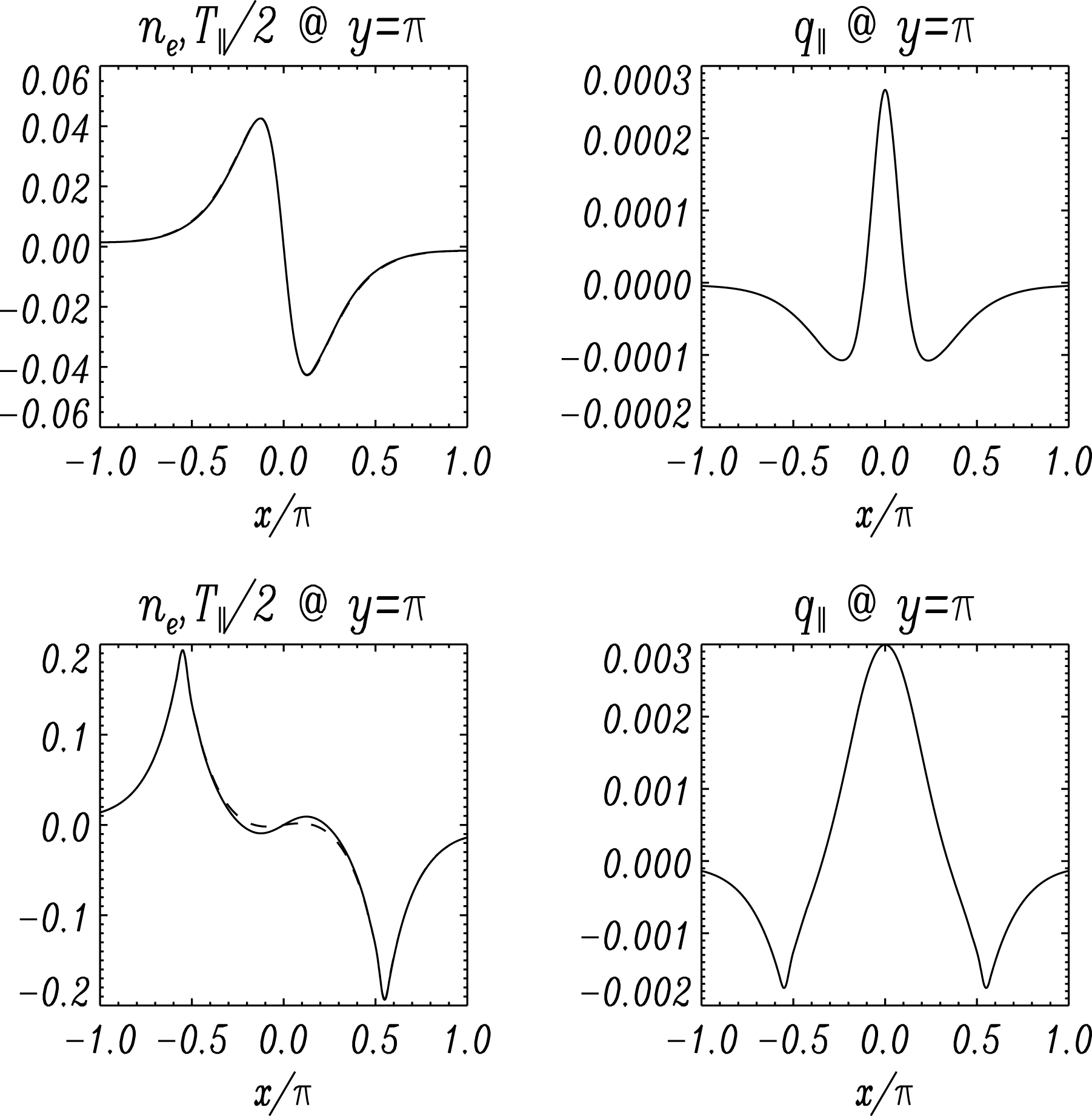
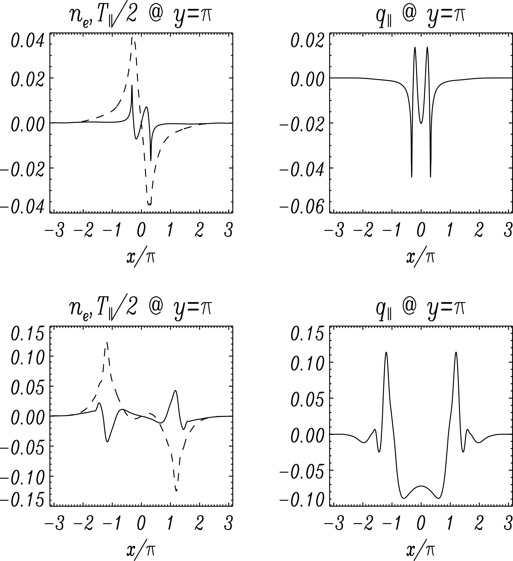
we expect the heat flux evolution to be not trivial. As a consequence, density and temperature fluctuations are no longer proportional. We illustrate this behaviour with the support of the numerical simulations. An example is given in figures 3 and 4, where in the left-hand panels we plot the profiles at
 $y={\rm\pi}$
, for two different simulation times, of the electron density fluctuations and of half the parallel temperature fluctuations for two cases with
 ${\it\rho}_{s}=0.01$
and
 ${\it\rho}_{s}=0.4$
, respectively. The simulation times are chosen for both cases in the nonlinear phase and close to saturation. We see that for small values of
 ${\it\rho}_{s}$
(figure 3) the two curves of
 $n_{e}$
and
 $T_{\Vert }/2$
are indistinguishable in the nonlinear phase and almost overlap at saturation as well. On the contrary for
 ${\it\rho}_{s}=0.4$
(figure 4) the density fluctuations are much larger than those of
 $T_{\Vert }/2$
. In particular, the greatest differences occur in regions where the heat flux fluctuations, shown in the right-hand panel of the same figure, become more pronounced. We observe in particular two positive peaks in
 $q_{\Vert }$
, which move further apart in time. It turns out that these peaks are located in correspondence with the magnetic island separatrices. Their drift in opposite directions indicates that the peaks are following the separatrices of the growing magnetic island. Further simulations suggest this behaviour to be quite generic for sufficiently large
 ${\it\rho}_{s}$
. Therefore, we can expect heat flux effects, when relevant, to be concentrated along the island separatrices rather than inside the island.
Figures on the left-hand side show profiles at
 $y={\rm\pi}$
of fluctuations of the electron density
 $n_{e}$
(dashed lines) superimposed to those of half the electron temperature
 $T_{\Vert }/2$
(solid lines). The figures on the right-hand side show the profiles at
 $y={\rm\pi}$
of the heat flux fluctuations
 $q_{\Vert }$
. All figures refer to the case
 ${\it\rho}_{s}=0.01$
. The first row corresponds to
 $t=325{\it\tau}_{A}$
, a simulation time in the nonlinear phase, and the second row corresponds to
 $t=400{\it\tau}_{A}$
, close to saturation. We indicate with
 ${\it\tau}_{A}=L/v_{A}$
the characteristic Alfvén time. In this regime the heat flux fluctuations remain negligible and temperature fluctuations are almost proportional to density fluctuations.

The meaning of the figures is the same as in figure 3, but here the case
 ${\it\rho}_{s}=0.4$
is shown. The first row corresponds to
 $t=250{\it\tau}_{A}$
, a simulation time in the nonlinear phase, and the second row corresponds to
 $t=325{\it\tau}_{A}$
, close to saturation. By comparing with figure 3, we observe that increasing
 ${\it\rho}_{s}$
leads to an increase in the heat flux. The highest peaks in the heat flux turn out to be located in correspondence with the island separatrices. As a consequence, temperature fluctuations no longer follow density fluctuations.

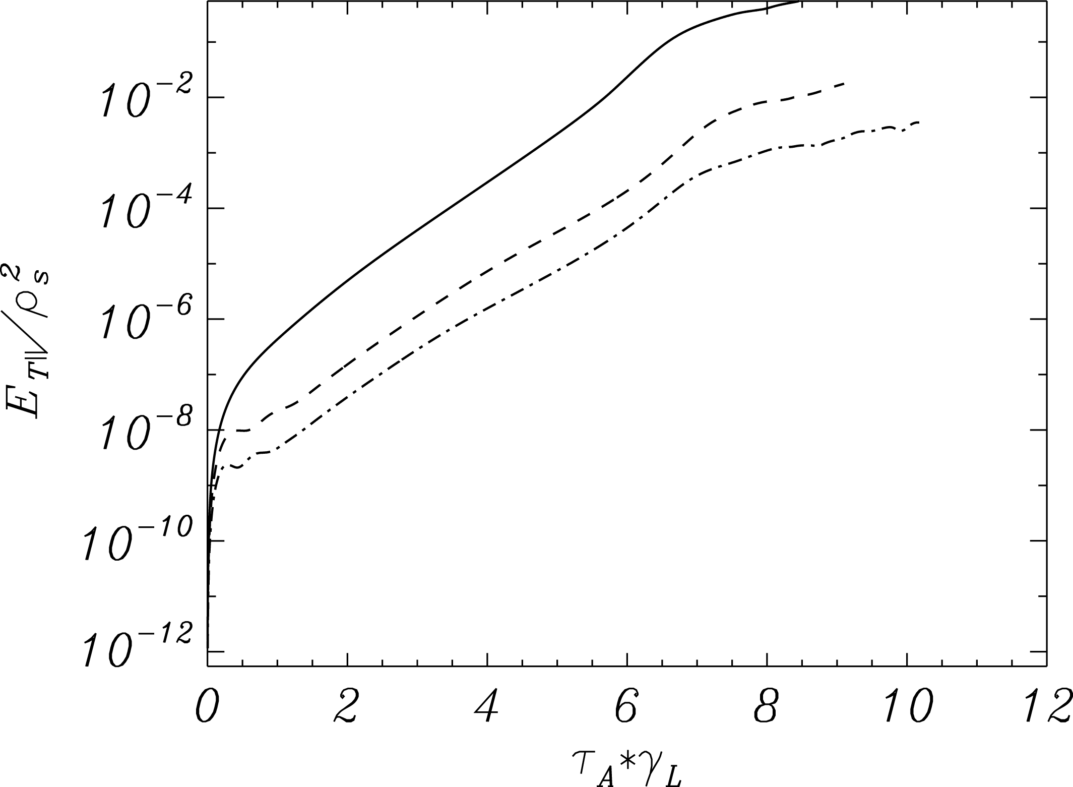
When we examine the role of high values of the ion sound Larmor radius we observe a tendency toward the suppression of temperature fluctuations. This behaviour is illustrated through the evolution of the integral quantity
 $2E_{T_{\Vert }}/{\it\rho}_{s}^{2}=\int \text{d}^{2}xT_{\Vert }^{2}/2$
in figure 5. We see that between the small- and the large-
 ${\it\rho}_{s}$
limits there are approximately three orders of magnitude of difference in the temperature fluctuations. As expected, then, heat flux contributes to distribute the temperature uniformly in space, which reflects into a reduction of temperature fluctuations.
Evolution in time of the energy associated with the parallel temperature variations for three different values of
 ${\it\rho}_{s}$
;
 ${\it\rho}=0.01$
(solid line),
 ${\it\rho}_{s}=0.4$
(dashed line) and
 ${\it\rho}_{s}=0.8$
(dash-dotted line). We observe that triggering heat flux, by increasing the value of
 ${\it\rho}_{s}$
, implies a reduction of temperature fluctuations.

The spatial distribution of temperature fluctuations in the smallest and largest
 ${\it\rho}_{s}$
cases can be observed from the contour plots shown in figure 6. In the small-
 ${\it\rho}_{s}$
limit small-scale structures are aligned with the magnetic island separatrix. An identical distribution is observed in the contour plots of
 $n_{e}$
(figure 8
a,b) and agrees with previous studies of the two-field model of Cafaro et al. (Reference Cafaro, Grasso, Pegoraro, Porcelli and Saluzzi1998), where density fluctuations were proportional to vorticity fluctuations. In the large-
 ${\it\rho}_{s}$
limit, as already noticed, the heat flux breaks the proportionality between
 $n_{e}$
and
 $T_{\Vert }/2$
. Whereas the former remains mainly concentrated along the separatrices, little energy is available for temperature fluctuations, which tend to be uniformly distributed inside the island.
Contour plot of the parallel temperature fluctuations
 $T_{\Vert }$
for
 ${\it\rho}_{s}=0.01$
(a) and
 ${\it\rho}_{s}=0.8$
(b). For
 ${\it\rho}_{s}\ll d_{e}$
,
 $T_{\Vert }$
distributes along the separatrices, similarly to
 $n_{e}$
(compare with figure 8
a). For larger
 ${\it\rho}_{s}$
, temperature fluctuations reduce and distribute more uniformly inside the island.

6. Role of the Lagrangian invariants
In this section we investigate the role, in the reconnection process, of the Lagrangian invariants of the model, introduced in § 3. The Lagrangian invariant dynamics underlying collisionless reconnection has already been exploited in two-, three- and four-field models for Hamiltonian reconnection such as those studied in Cafaro et al. (Reference Cafaro, Grasso, Pegoraro, Porcelli and Saluzzi1998), Grasso et al. (Reference Grasso, Califano, Pegoraro and Porcelli2001, Reference Grasso, Borgogno, Pegoraro and Tassi2009, Reference Grasso, Tassi and Waelbroeck2010) and Comisso et al. (Reference Comisso, Grasso, Tassi and Waelbroeck2012). In all of these models some field variables (typically densities, parallel canonical momenta or vorticity) could be expressed as linear combinations of two Lagrangian invariants associated with Casimirs of the corresponding Poisson brackets. The dynamics of the Lagrangian invariants could then be used as a viewpoint alternative to that of the original field variables. The inclusion of parallel temperature and heat flux fluctuations in the six-field model extends this picture. Indeed, by inverting the relations (3.16)–(3.19), one obtains
 $$\begin{eqnarray}\displaystyle & \displaystyle n_{e}=-\frac{G_{1}-G_{2}-(\sqrt{2}+\sqrt{3})(G_{3}-G_{4})}{4\sqrt{3+\sqrt{6}}d_{e}{\it\rho}_{s}}, & \displaystyle\end{eqnarray}$$
 $$\begin{eqnarray}\displaystyle & \displaystyle F=\frac{G_{1}+G_{2}+G_{3}+G_{4}}{4}, & \displaystyle\end{eqnarray}$$
 $$\begin{eqnarray}\displaystyle & \displaystyle T_{\Vert }=-\frac{(\sqrt{2}+\sqrt{3})(G_{1}-G_{2})+G_{3}-G_{4}}{2\sqrt{2}\sqrt{3+\sqrt{6}}d_{e}{\it\rho}_{s}}, & \displaystyle\end{eqnarray}$$
 $$\begin{eqnarray}\displaystyle & \displaystyle q_{\Vert }=-\sqrt{3}\frac{G_{1}+G_{2}-G_{3}-G_{4}}{4\sqrt{2}d_{e}^{2}}, & \displaystyle\end{eqnarray}$$
 $$\begin{eqnarray}\displaystyle & \displaystyle n_{i}=\frac{I_{+}-I_{-}}{2d_{i}{\it\rho}_{i}}, & \displaystyle\end{eqnarray}$$
 $$\begin{eqnarray}\displaystyle & \displaystyle D=\frac{I_{+}+I_{-}}{2d_{i}{\it\rho}_{i}}. & \displaystyle\end{eqnarray}$$
 $n_{i}$
and
 $D$
remain linear combinations of two contributions
 $I_{\pm }$
, as in the four-field model (Waelbroeck & Tassi Reference Waelbroeck and Tassi2012). The four electron fields, on the other hand, are all linear combinations of the four Lagrangian invariants
 $G_{1}$
,
 $G_{2}$
,
 $G_{3}$
and
 $G_{4}$
. In particular, we remark that
 $n_{e}$
and
 $T_{\Vert }$
can be seen as linear combinations of the two fields
 $G_{1}-G_{2}$
and
 $G_{3}-G_{4}$
, weighted with different coefficients. On the other hand,
 $F$
and
 $q_{\Vert }$
can be seen as linear combinations of the two fields
 $G_{1}+G_{2}$
and
 $G_{3}+G_{4}$
. Such two fields contribute to
 $F$
and
 $q_{\Vert }$
with the same weight (up to the sign).
We observe that the field variables also possess discrete symmetries. The symmetries for the even-order moments
 $n_{e}$
,
 $T_{\Vert }$
and
 $n_{i}$
are
 $$\begin{eqnarray}n_{e}(-x,y,t)=-n_{e}(x,y,t),\quad n_{e}(x,-y,t)=-n_{e}(x,y,t),\end{eqnarray}$$
 $$\begin{eqnarray}\displaystyle & \displaystyle T_{\Vert }(-x,y,t)=-T_{\Vert }(x,y,t),\quad T_{\Vert }(x,-y,t)=-T_{\Vert }(x,y,t), & \displaystyle\end{eqnarray}$$
 $$\begin{eqnarray}n_{i}(-x,y,t)=-n_{i}(x,y,t),\quad n_{i}(x,-y,t)=-n_{i}(x,y,t),\end{eqnarray}$$
whereas the symmetries for the odd-order moments are
 $$\begin{eqnarray}F(-x,y,t)=F(x,y,t),\quad F(x,-y,t)=F(x,y,t),\end{eqnarray}$$
 $$\begin{eqnarray}\displaystyle & \displaystyle q_{\Vert }(-x,y,t)=q_{\Vert }(x,y,t),\quad q_{\Vert }(x,-y,t)=q_{\Vert }(x,y,t), & \displaystyle\end{eqnarray}$$
 $$\begin{eqnarray}D(-x,y,t)=D(x,y,t),\quad D(x,-y,t)=D(x,y,t).\end{eqnarray}$$
Such symmetries, through the linear combinations (3.16)–(3.20), are reflected in the following relations between the Lagrangian invariants:
 $$\begin{eqnarray}G_{1}(-x,y,t)=G_{2}(x,y,t),\quad G_{1}(x,-y,t)=G_{2}(x,y,t),\end{eqnarray}$$
 $$\begin{eqnarray}G_{3}(-x,y,t)=G_{4}(x,y,t),\quad G_{3}(x,-y,t)=G_{4}(x,y,t),\end{eqnarray}$$
 $$\begin{eqnarray}I_{+}(-x,y,t)=I_{-}(x,y,t),\quad I_{+}(x,-y,t)=I_{-}(x,y,t).\end{eqnarray}$$
In Comisso et al. (Reference Comisso, Grasso, Tassi and Waelbroeck2012), simulations of the four-field model showed that the two Lagrangian invariants associated with the electron fluid tend to rotate in opposite directions, under the action of stream functions analogous to those of (3.22). For the Lagrangian invariants associated with the ion fluid, the rotations were greatly reduced as a consequence of the mass ratio. In the six-field model we confirm, without showing it, the same behaviour with regard to the ion variables
 $n_{i}$
and
 $D$
. We focus then on the electron field variables, whose dynamics can be equivalently described by that of the Lagrangian invariants
 $G_{1}$
,
 $G_{2}$
,
 $G_{3}$
and
 $G_{4}$
, following equations (6.1)–(6.4). In figure 7, contour plots of the Lagrangian invariants
 $G_{1}$
and
 $G_{3}$
are shown (the contour plots of
 $G_{2}$
and
 $G_{4}$
can be obtained by reflection exploiting the symmetry properties discussed above). By looking in particular at the contour plot, for
 ${\it\rho}_{s}=0.8$
, of
 $G_{3,4}$
, one observes two sorts of spiral arms, which turn out to be essentially aligned with the island separatrices. These spiral arms are the result of a rotation of
 $G_{3,4}$
induced by the stream function
 ${\it\phi}_{3,4}$
. Analogously,
 $G_{1,2}$
rotate in opposite directions under the action of the stream functions
 ${\it\phi}_{1,2}$
. For the case
 ${\it\rho}_{s}=0.01$
, the rotations in opposite directions are essentially negligible because for
 ${\it\rho}_{s}\ll d_{e}$
one has
 ${\it\phi}_{1,2,3,4}\approx {\it\phi}$
.
Contour plots of the invariants
 $G_{1,3}$
for
 ${\it\rho}_{s}=0.01$
(a,c) and
 ${\it\rho}_{s}=0.8$
(b,d). For
 ${\it\rho}_{s}=0.8$
, one can observe in the plot of
 $G_{3}$
the presence of two spiral arms, which are a signature of the rotation of the Lagrangian invariant. For
 ${\it\rho}_{s}=0.01$
, rotations in opposite directions of the two pairs of Lagrangian invariants tend to be suppressed.

We can then reinterpret qualitative features of field structures in terms of the Lagrangian invariants. For the parallel temperature, for instance, the rotation of the invariants for
 ${\it\rho}_{s}=0.8$
leads to the homogenization of the fluctuations inside the island, as observed in figure 6. The absence of rotation for the case
 ${\it\rho}_{s}=0.01$
, on the contrary, leads to the persistence of structures clearly aligned with the island separatrix.
As above observed, the electron density is also given by a linear combination of
 $G_{1}-G_{2}$
and
 $G_{3}-G_{4}$
, as the parallel temperature, but with different coefficients. Whereas for
 $T_{\Vert }$
the dominating contribution in the linear combination is
 $G_{1}-G_{2}$
, for the density it comes from
 $G_{3}-G_{4}$
, which is multiplied by the greater coefficient (and also subtracted). This reflects in the electron density not having small-scale structures inside the island for
 ${\it\rho}_{s}=0.8$
(see figure 8), unlike
 $T_{\Vert }$
. The absence of rotation for
 ${\it\rho}_{s}=0.01$
amounts to yielding the same structures for
 $n_{e}$
and
 $T_{\Vert }$
, which corresponds, as observed in § 5, to negligible heat flux.
Contour plots of the electron density fluctuations
 $n_{e}$
for
 ${\it\rho}_{s}=0.01$
(a) and
 ${\it\rho}_{s}=0.8$
(b). The distribution of the density fluctuations can be obtained as a superposition of those of
 $G_{1}-G_{2}$
and
 $G_{3}-G_{4}$
, according to (6.1).

The qualitative structures of the heat flux fluctuations can also be reinterpreted in terms of the Lagrangian invariants. We recall that in § 5 we remarked that
 $q_{\Vert }$
, when non-negligible, exhibits peaks around the separatrices. This can also be observed in figure 9 in the case
 ${\it\rho}_{s}=0.8$
. Such peaks reflect the superposition of the spiral arms of the invariants
 $G_{1,2,3,4}$
formed as a consequence of their rotation. When the rotation is essentially absent, as is the case for
 ${\it\rho}_{s}=0.01$
, such peaks are not present and the little amount of energy in the heat flux fluctuations is concentrated, to a large extent, also inside the island around the resonant surface
 $x=0$
.
Contour plots of the heat flux fluctuations
 $q_{\Vert }$
for
 ${\it\rho}_{s}=0.01$
(a) and
 ${\it\rho}_{s}=0.8$
(b). Heat flux structures can be obtained as a superposition of the structures of
 $G_{1}+G_{2}$
and
 $G_{3}+G_{4}$
according to (6.4). We note in particular the concentration along the separatrices, as a result of the opposite rotations of the Lagrangian invariants in the case
 ${\it\rho}_{s}=0.8$
.

7. Conclusions
We considered a six-field fluid model for collisionless reconnection accounting for electron parallel temperature and heat flux dynamics. The model extends previous Hamiltonian reconnection models (Cafaro et al.
Reference Cafaro, Grasso, Pegoraro, Porcelli and Saluzzi1998; Waelbroeck et al.
Reference Waelbroeck, Hazeltine and Morrison2009; Waelbroeck & Tassi Reference Waelbroeck and Tassi2012) based on an isothermal closure. We showed that, like its isothermal predecessors, the six-field model also possesses a Hamiltonian structure with a non-canonical Poisson bracket. With regard to this point we mention that conservation of the total energy (the Hamiltonian functional) for the six-field model was already evident from Scott (Reference Scott2010). Also, the property of energy conservation of the six-field model is compatible with the analysis of Hammett et al. (Reference Hammett, Beer, Dorland, Cowley and Smith1993). In this reference it is indeed pointed out that fluid models evolving a finite number
 $\mathscr{N}$
of moments of the Vlasov distribution function with respect to Hermite polynomials of the velocity coordinate conserve energy if the hierarchy of fluid equations is closed by setting the moment of order
 $\mathscr{N}+1$
equal to zero. The six-field model can actually be shown to admit a derivation from gyrokinetic equations by taking moments with respect to Hermite polynomials (Scott Reference Scott2010) in the parallel velocity coordinate, and imposing the fourth-order moment to be zero. In this paper we have shown that the model, in addition to being energy-conserving, possesses the stronger property of being Hamiltonian. In particular, the non-canonical nature of the Poisson bracket implies, in addition to energy conservation, the existence of an infinite number of conserved functionals, corresponding to the Casimirs (3.14) and (3.15). Similarly to what occurred for the isothermal models (Cafaro et al.
Reference Cafaro, Grasso, Pegoraro, Porcelli and Saluzzi1998; Waelbroeck et al.
Reference Waelbroeck, Hazeltine and Morrison2009; Waelbroeck & Tassi Reference Waelbroeck and Tassi2012), also in the six-field model then, in spite of the violation of the conservation of the topology of the magnetic field, alternative topological conservation laws constrain the dynamics. All contour lines of the Lagrangian invariants
 $G_{1,2,3,4},I_{\pm }$
are indeed conserved, in spite of reconnection of magnetic field lines.
By means of numerical simulations we have observed that, when compared to the isothermal four-field model (Comisso et al.
Reference Comisso, Grasso, Tassi and Waelbroeck2012), the six-field model yields, in the large-
 ${\it\Delta}^{\prime }$
regime, slightly greater linear growth rates, but essentially the same island saturation amplitudes, in agreement with hybrid fluid/kinetic models (Loureiro et al.
Reference Loureiro, Schekochihin and Zocco2013). In this respect, the effect of the heat flux on the reconnection process seems not to be considerable, at least for a plasma with no density or temperature equilibrium gradients, such as that considered in this paper.
Heat flux and parallel temperature offer new forms where energy can be converted to, when compared with the isothermal models. Indeed, we observed that temperature and heat flux fluctuations gain energy at the expense of electron thermal, electrostatic and parallel kinetic energies.
We also investigated the dynamics of the six-field model as a function of the
 ${\it\rho}_{s}$
parameter (or, equivalently, of the
 ${\it\beta}_{e}$
parameter). For
 ${\it\rho}_{s}\ll d_{e}$
, heat flux is negligible and consequently temperature fluctuations tend to go in phase with density fluctuations. In particular, they both concentrate along the island separatrices. Increasing the value of
 ${\it\rho}_{s}$
triggers heat flux fluctuations, which, as expected, act to damp temperature fluctuations. The latter, in particular, tend to distribute more uniformly inside the island. This occurs as a consequence of heat flux distributing along the separatrices. Density fluctuations, too, still exhibit a considerable concentration along the separatrices.
The field structures can also be qualitatively reinterpreted in terms of the Lagrangian invariants as done in Cafaro et al. (Reference Cafaro, Grasso, Pegoraro, Porcelli and Saluzzi1998), Grasso et al. (Reference Grasso, Califano, Pegoraro and Porcelli2001) and Comisso et al. (Reference Comisso, Grasso, Tassi and Waelbroeck2012). In particular, it emerged that the four electron variables
 $n_{e}$
,
 $F$
,
 $T_{\Vert }$
and
 $q_{\Vert }$
organize in pairs according to their discrete symmetry properties. The variables
 $n_{e}$
and
 $T_{\Vert }$
, which are odd functions, appear as linear combinations of
 $G_{1}-G_{2}$
and
 $G_{3}-G_{4}$
. On the other hand, the even fields
 $F$
and
 $q_{\Vert }$
are proportional to the sum and the difference, respectively, of
 $G_{1}+G_{2}$
and
 $G_{3}+G_{4}$
. Rotation of the Lagrangian invariants
 $G_{1,2,3,4}$
is observed, as was the case for the Lagrangian invariants of isothermal models. In particular, for large
 ${\it\rho}_{s}$
, the rotation induces the formation of structures similar to spiral arms, along the separatrices, in
 $G_{3}$
and
 $G_{4}$
. For
 ${\it\rho}_{s}\ll d_{e}$
, on the other hand, little stretching of the invariants is observed, due to the negligible influence of the magnetic potential in the advecting stream functions
 ${\it\phi}_{1,2,3,4}$
. The above-mentioned features of the field structures, such as the concentration of density and heat flux along the separatrices, can then be seen as the superposition of the Lagrangian invariants undergoing more or less intense stretching depending on the value of
 ${\it\rho}_{s}$
. Rotation of the Lagrangian invariants had already been observed for the Hamiltonian isothermal models (Cafaro et al.
Reference Cafaro, Grasso, Pegoraro, Porcelli and Saluzzi1998; Grasso et al.
Reference Grasso, Califano, Pegoraro and Porcelli2001; Comisso et al.
Reference Comisso, Grasso, Tassi and Waelbroeck2012) and drift-kinetic systems (Liseikina et al.
Reference Liseikina, Pegoraro and Echkina2004; Pegoraro et al.
Reference Pegoraro, Liseikina and Echkina2005a
,Reference Pegoraro, Liseikina and Echkina
b
). Our analysis shows that this feature persists when including parallel temperature and heat flux effects while preserving the Hamiltonian structure of the model.
Acknowledgements
E.T. acknowledges financial support from the Agence Nationale de la Recherche (ANR GYPSI n. 2010 BLAN 941 03) and from the CNRS through the PEPS project GEOPLASMA 2.