1. Introduction
Among developing countries, many West African countries are seen as the most vulnerable to climate shocks. These shocks do not only include potentially catastrophic large-scale disasters, but also testify to a more permanent state of economic stress which results from higher average temperatures, reduced availability of water sources, more frequent flooding and intensified windstorms (UNDP, 2004). Moreover, the burden of adjusting to the threats from climate shocks is heaviest for those economies. Indeed, they have already suffered what is known as ‘multiple vulnerabilities’ because of their low level of resilience to shocks (Guillaumont, Reference Guillaumont2009).
A recent literature has analyzed the impact of climate shocks and natural disasters in order to assess their contribution to the volatility of GDP in developing countries (Raddatz, Reference Raddatz2007; Hochrainer, Reference Hochrainer2009; Loayza et al., Reference Loayza, Olaberria, Rigolini and Christiaensen2009) Results show that the macroeconomic performance of developing countries is highly exposed to climate shocks, and especially to droughts in the short term.Footnote 1 Other contributions have shown how population may use migration and remittances in order to cope with the negative impacts of bad weather conditions (Findley, Reference Findley1994; Ebeke and Combes, Reference Ebeke and Combes2013).
Although it is now widely recognized that remittance inflows may benefit households at a microeconomic level (Gupta et al., Reference Gupta, Pattillo and Wagh2009), their empirical macroeconomic consequences remain less investigated (Rapoport and Docquier, Reference Rapoport and Docquier2005) and few studies have highlighted their countercyclical role in mitigating the effects of negative shocks (IMF, 2005; Ebeke and Combes, Reference Ebeke and Combes2013). Indeed, the consequences of remittances depend on whether they are consumed or invested (Ratha, Reference Ratha2007). They are expected to have either direct positive effects, when they directly contribute to productive investments, or indirect effects, when they are used by households to consume goods and services produced locally. Otherwise, if they result in demand exceeding domestic production capacities, they may spur imports, and especially imports of agricultural goods, in order to satisfy new consumption habits or to maintain a vital level of consumption (Jovi
 ić and Mitrović, Reference Jovic̃ić and Mitrović2006).
This paper parallels these issues by investigating the impact of remittances on macroeconomic performance in West African countries undergoing climate stress. Accordingly, we estimate the relationship between droughts, remittances and economic performance for a sample of eight West African countries over the period 1985–2007, relying on a panel conditional homogeneous vector autoregressive (PCHVAR) model, which has the advantage (i) of exploiting the panel nature of the data and (ii) of shaping heterogeneities in countries’ dynamics conditionally to an exogenous variable (Georgiadis, Reference Georgiadis2012).
Our analysis is distinct of the existing literature in many respects. First, we seek to identify the direct impact of remittances on macroeconomic performance and their indirect impact through their financial deepening effect. Secondly, the role of remittances is assessed by taking into account potential non-linearities and heterogeneities caused by climatic conditions of West African economies. Finally, we focus on climate stress through the computation of the standardized precipitation index (SPI) by using precipitation data from the Climate Research Unit (CRU). This index allows us to assess more accurately the impact of a purely physical shock, compared to proxies of climate shocks widely used in the literature.
The main results of this paper are the following. First, remittances do not exert spillover effects on the agricultural value added and tend instead to increase agricultural imports, especially when countries face negative rainfall shocks. Secondly, our findings show that remittances may have a positive effect on financial development only when cumulative precipitation deviates positively from the climatological average. This relationship becomes negative in case of stress conditions such as droughts. Finally, we find a negative impact of financial development on GDP per capita, pointing out the lack of complementarity between remittances, financial development and growth.
The remainder of the paper is organized as follows. Section 2 outlines the empirical literature dealing with the impact of remittances on macroeconomic performance in developing countries. In section 3, we present the design of the PCHVAR model employed in this paper. In section 4, we describe the data and the empirical specification of the model. Section 5 displays our different results. Finally, section 6 concludes.
2. Literature review
Regional and international population mobility has a major impact on economic development in West Africa (De Haas, Reference De Haas2010). Recent migration patterns and their causes are linked to multiples forces, among which remittances constitute a ‘bond’ connecting migrants to their families. Between 1996 and 2009, West African countries received 30 per cent of the official remittances sent to sub-Saharan African countries. Their share in the regional GDP has averaged 3.2 per cent over the same period and rose from 2.1 per cent to 4.3 per cent in 2009.Footnote 2
Several theoretical and empirical studies initiated by the New Economics of Labor Migration (Lucas and Stark, Reference Lucas and Stark1985) show that migration and remittances are an integral part of a household's risk management strategies. According to, Findley (Reference Findley1994) during the great drought (1984–1985), 63 per cent of agricultural households in Mali depended on remittances sent by non-resident family members abroad, suggesting the importance of those transfers as a means of providing insurance against climate hazards. In theory, droughts should negatively affect the income of households predominantly occupied in the agricultural sector, and we may therefore expect remittance inflows to support basic consumption and/or productive investments.
The question of whether remittances inflows have beneficial or detrimental effects on economic development is the subject of an extensive literature, and of a controversial debate. It has mainly focused on how remittances are used, i.e., whether they are mainly consumed or spent in productive investment.
The multiplier effect exerted by remittances on national income can only take place in a context where the additional demand induced by remittances inflows can be satisfied by domestic production. In that case, a share of those transfers is injected into the economy through productive investment. On the contrary, if remittances cannot be absorbed by domestic production, their multiplier effect will be severely limited (Glytsos, Reference Glytsos1993). Empirical studies fail to reach clear-cut results at a microeconomic level. They show that remittances can foster productive investments but also allow households to maintain consumption through a process of intertemporal smoothing.
Adams (Reference Adams2002) finds that Pakistani households receiving international remittances have a greater saving propensity than households benefiting from a pension. According to Taylor (Reference Taylor1999), remittances serve as insurance against risks associated with new production activities. According to Lucas and Stark (Reference Lucas and Stark1985), remittances tend to reduce labor supply and cereal production in the short run in sub-Saharan Africa, whereas in the long run, they are invested and thus promote cereal productivity and livestock accumulation. Yang and Choi (Reference Yang and Choi2005), testing the role of remittances in insuring against rainfall shocks in the Philippines, show that 60 per cent of the households’ income loss due to these shocks is offset by remittances, which help consumption to stabilize. Remittances can also stimulate subsistence consumption if the income of households is below a certain threshold after a negative shock (Yang, Reference Yang2008). Similar behavior is displayed when households are facing a crisis or a shock pressuring their previous level of consumption. Case studies undertaken on Mali, Senegal, Morocco and the Comoros (IFDA, 2009) show that only 10 per cent of the households receiving remittances used them for productive investments. Those findings support the conclusion reached by Chami et al. (Reference Chami, Fullenkamp and Jahjah2003) that rural households tend to rely heavily on remittances to improve their living conditions through the satisfaction of basic needs.
The fact that households use remittances to smooth consumption raises the question of whether additional demand induced by remittances may be satisfied by domestic production. Indeed, if demand rises without a stimulation of the supply side, remittances can foster an increase in imports and then lead to a deterioration of the trade balance. Furthermore, when imports financed by remittances involve basic necessities, their multiplier effect is small. Thus, although remittances can tackle risks of increasing poverty, they cannot necessarily allow countries to be more resilient to future shocks if they spur imports.
Recently, studies examining the role of remittances on economic development have underlined their effect on growth through their interaction with financial development. These studies are also debated and reach different conclusions (Aggarwal et al., Reference Aggarwal, Demirgüç-Kunt and Pería2011). According to Mundaca (Reference Mundaca2005) and Ahamada and Coulibaly (Reference Ahamada and Coulibaly2011), remittances may be better used in countries showing high financial development, and they may thus have a positive effect on growth. Therefore, large remittances inflows could have non-significant or smaller effects on growth in less financially developed countries.
However, remittances may also promote growth in such countries. Indeed, they may compensate for the lack of financial markets in rural areas by easing liquidity constraints and supporting productive investment. In this case, remittances are assumed to promote growth in less financially developed countries (Giuliano and Ruiz-Arranz, Reference Giuliano and Ruiz-Arranz2009). Finally, remittances can help foster financial development in developing countries (Demirgüç-Kunt et al., Reference Demirgüç-Kunt, Detragiache and Merrouche2010; Aggarwal et al., Reference Aggarwal, Demirgüç-Kunt and Pería2011).
3. Methodology: the PCHVAR specification
In order to analyze the multiple causality and spillover effects between remittances and economic performance in a context of climate shocks, we use a PCHVAR model which extends the traditional panel vector autoregressive (PVAR) model. The PCHVAR model offers several advantages, by allowing for unobserved individual heterogeneity, cross-section dependency and exogenous conditioning variables.
The dynamics in standard PVAR frameworks are assumed to be fully homogeneous across cross-sectional units. This assumption is usually maintained for the sake of parsimony and to gain degrees of freedom by pooling the data of cross-sectional units. However, this restriction may not hold in a macroeconomic setting since countries may be subject to asymmetrical shocks, and may implement different policy measures and/or responses to cope with those shocks (Canova and Ciccarelli, Reference Canova and Ciccarelli2013).
In this case, using fixed effects to allow heterogeneity between the panels’ units may be problematic since OLS and standard fixed effect estimators (LSDV) are known to be biased in panels that include lagged endogenous variables (Holtz-Eakin, Reference Holtz-Eakin1988). Even if this problem is eliminated when the time dimension T is relatively large compared to the cross-sectional dimension N (T > 2N), OLS and LSDV estimations can still show bias when the time dimension is large if the coefficients on the lagged endogenous variables vary greatly across countries.
Macroeconomic studies have made extensive use of generalized method of moments (GMM) techniques in order to estimate panel VARs. By employing a forward orthogonal deviations transformation so as to eliminate time-invariant individual fixed effects, lagged level variables can be thus used as instruments in GMM estimations (Love and Zicchino, Reference Love and Zicchino2006). However, GMM and extended GMM estimators are designed for the case of a large cross-sectional dimension (N) relative to the time dimension (T) and have been shown to perform poorly when T → ∞ and particularly when the ratio of the variance of the individual effects to the variance of the innovations increases (Juessen and Linnemann, Reference Juessen and Linnemann2012).
To address these concerns, we then set up a PCHVAR model, allowing for heterogeneous cross-sectional dynamics (Georgiadis, Reference Georgiadis2012):
 $$Y_{it} = \sum_{j=1}^p A_j\lpar z_{it}\rpar Y_{i\comma t-j} + \delta_i + B_q w_{t-q} + \varepsilon_{it} \quad \varepsilon_{it} i.i.d. \ \lpar 0\comma \; \Sigma_\varepsilon\rpar$$
where Y it , the vector of five endogenous regressors, comprises the real GDP (PPP adjusted) per capita (y), the agricultural value added per capita (y agr ), remittances and compensation of employee per capita inflows (R i ), agricultural imports per capita (M agr ) and a financial sector development index (F d ). z it is a M × 1 matrix of exogenous variables comprising the drought probability index; δ i is a d × 1 vector of fixed effect and unit-specific time trend; and w t , a L × 1 vector of exogenous variable affecting all countries at the same time (homogeneous effect), comprises the GDP per capita of developed countries.Footnote 3
Unlike the standard Panel VAR, the PCHVAR model allows for different cross-sectional dynamics. The time series are pooled, but impulse responses differ based on the values of one exogenous conditioning variable z it . Assuming that each scalar coefficient a j, sm in the matrix of coefficients A j can be approximated by a scalar polynomial in the conditioning exogenous variable z it (with j = 1, …, p, s = 1, …, K and m = 1, …, K):
 $$a_{j\comma sm}\lpar z_{it}\rpar \approx \pi\lpar z_{it}\rpar \gamma_{j\comma sm}$$
with π(z it ) = [π1(z it ), π2(z it ), …, πτ (z it )] is a vector with polynomials in (z it ) and γ j,sm = (γ j,sm 1 , γ j,sm 2 , …, γ j,sm τ ) is a vector of polynomial coefficients. A j (.) can then be rewritten:
 $$\eqalign{A_j\lpar z_{it}\rpar &= \left[\matrix{\pi\lpar z_{it}\rpar \cdot \gamma_{j\comma 11} \hfill &\cdots \hfill & \pi\lpar z_{it}\rpar \cdot \gamma_{j\comma 1K} \cr \hfill \vdots \hfill &\ddots \hfill &\vdots \cr \pi\lpar z_{it}\rpar \cdot \gamma_{j\comma K1} \hfill &\cdots \hfill &\pi\lpar z_{it}\rpar \cdot \gamma_{j\comma KK} } \right]\cr &= \left[\matrix {\gamma_{j\comma 11}^\prime \hfill & \cdots \hfill & \gamma_{j\comma 1K}^\prime \cr \hfill \vdots \hfill & \ddots \hfill & \vdots \cr \gamma_{j\comma K1}^\prime \hfill &\cdots \hfill & \gamma_{j\comma KK}^\prime} \right]\cdot \lsqb I_K \otimes \pi^\prime \lpar z_{it}\rpar \rsqb \cr & = \Gamma_j \cdot \lsqb I_K \otimes \pi^\prime \lpar z_{it}\rpar \rsqb .}$$
The model in equation (1) can be written as follows:
 $$Y_{it} = \sum_{j=1}^{p}\Gamma_j \cdot \lsqb I_K \otimes \pi^\prime \lpar z_{it}\rpar \rsqb Y_{i\comma t - j} + \delta_i + B_qw_{t-q} + \varepsilon_{it}$$
 $$= \sum_{j=1}^{p} \Gamma_j \cdot x_{i\comma t-j} + \delta_i + B_qw_{t-q} + \varepsilon_{it}$$
 $$= \Gamma_j \cdot X_{i\comma t-1} + \delta_i + B_qw_{t-q} + \varepsilon_{it}.$$
Following Georgiadis (Reference Georgiadis2012), the model in equation (6) can be interpreted as a standard multiple equations panel time series model and is estimated using OLS. Once the polynomial coefficients in the matrix Γ are estimated, the reduced form coefficient matrix A j (·) is calculated for multiple values of the conditioning variable.
In cases of cross-section dependency across panels’ units, the model given by equation (6) may be estimated using the technique proposed by Pesaran (Reference Pesaran2006). Pesaran tackles the issue of cross-sectional dependency in a panel dynamics model by approximating the common component of the data by the cross-sectional averages of the dependent and explanatory variables, and then augmenting the panel regression with these averages.
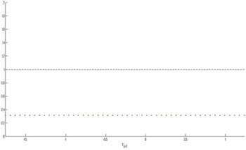
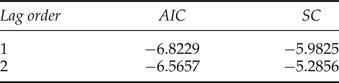
The lag order is chosen by minimizing the Akaike information criterion (AIC) and the Schwarz criterion (SC). In accordance with the AIC and SC results and the limited size of our sample, we include only one lag in the vector of endogenous regressors y it and in the vector of exogenous variables with homogeneous effects (w t ). A stability test indicates that the model given by equation (6) is stationary.Footnote 4 Once the unknown parameters are estimated, dynamic simulations can be performed as orthogonalized impulse response functions (OIRFs), as well as forecast error variance decompositions (FEVD), allowing for the examination of the impact which innovations or shocks affecting any particular variable have on other variables in the system.
Because of the dependence of the coefficient matrices on the conditioning variable A j (z it ), OIRFs and FEVD in the PCHVAR model are functions of the conditioning variable and are interpreted for a grid of values of the conditioning variable. To obtain OIRFs, we decompose the residuals in a way that makes them orthogonal, by adopting the Choleski decomposition. This decomposition involves a particular ordering of variables where the variables that appear earlier affect the following variables contemporaneously and with lags, while the variables that appear later only affect the previous variables with lag. The variables order in the vector of endogenous regressors is based upon the Granger causality test on panel data proposed by Emirmahmutoglu and Kose (Reference Emirmahmutoglu and Kose2011).
4. Estimation of the PCHVAR model
4.1. The sample
Given the availability of data, our study relies on annual data covering the 1985–2007 period and eight West African countries.Footnote 5 All data are log transformed. Real GDP per capita (PPP adjusted) is extracted from PennWorld tables. GDP per capita of developed countries (PPP adjusted), total agricultural imports per capita (current US$ ), agricultural value added per capita (constant US$ ), remittances and compensation of employee data come from the World Bank Development Indicators database (World Bank, 2013). Worker remittances and compensation of employees include current remittances by migrant workers, plus wages and salaries earned by non-resident workers. Per capita remittances are obtained by dividing the total amount of remittance inflows by the total population of each country.
Following Ahamada and Coulibaly (Reference Ahamada and Coulibaly2011) and Beck and Demirgüç-Kunt (Reference Beck and Demirgüç-Kunt2006) and, we use private credit by deposit money banks and other financial institutions as percentage of GDP as a measure of financial development. Data are extracted from the World Bank Global Financial Development Database (2013).Footnote 6
Several studies (Skidmore and Toya, Reference Skidmore and Toya2002; Raddatz, Reference Raddatz2007; Reference Raddatz2009) assess the impact of natural and climate disasters on the macroeconomic stability of developing countries using the International Disaster (EM-DAT) database developed by the Centre for Research on the Epidemiology of Disasters (CRED). However EM-DAT data show some limitations (UNDP, 2004). Firstly, such data do not take into account the potential correlation between shocks (a shock coming from another shock). Some climate shocks, like droughts, are also problematic because they tend to develop gradually over time and space. Thus, their occurrence and their economic impact cannot be approximated by a binary variable. Another limitation is related to the endogeneity problem inherent to the production of such data. Indeed, a disaster is defined by the number of people affected by the shock during a year. Thus, this measure relies on the ability or inability of individuals to cope with the shock and does not take into account the physical dimension of the shock. These various limits are closely related to the concept of disaster, which gives only limited importance to the temporal dimension of climate shocks.
Therefore, we propose to use rainfall data from the CRUFootnote 7 in order to measure the impact of shocks on remittances, since rainfall variability constitutes the primary source of income risk in many African countries (Gubert, Reference Gubert2002). Following McKee et al. (Reference McKee, Doesken and Kleist1993), we compute the Standardized Precipitation Index (SPI) with a six-month timescale.Footnote 8 The SPI is commonly used for defining and monitoring droughts. It captures the occurrence and the severity of droughts at a given timescale (temporal resolution) for any rainfall station with historical data and can also be used to determine periods of anomalous wet events. The SPI is the transformation of the precipitation time series into a standardized normal distribution (z-distribution) and has several advantages compared to other drought indicators such as the Palmer Drought Severity Index (PDSI). In particular, since the SPI uses normalized rainfall data and compares the current rainfall with the average, different areas with different rainfall characteristics can be compared in terms of how badly they are experiencing drought conditions (Edwards and McKee, Reference Edwards and McKee1997). The index is negative for drought, and positive for wet conditions. As the dry or wet conditions become more severe, the index tends to 3 or −3.
4.2. Unit roots, cointegration and causality tests
Climate shock occurrence in a specific country may have macroeconomic consequences in the neighboring countries. For instance, precipitation shocks in sending countries (such as Côte d'Ivoire) may reduce remittances inflows in receiving countries, and in turn affect overall economic performance. Similarly, climate shocks may reduce domestic production capacities and constrain exports to neighboring countries. Thus, the potential correlation between macroeconomic performance on a regional scale after a climate shock requires taking into account the dependence hypothesis between countries.
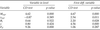
Results of the cross-sectional dependence (CD) test of Pesaran (Reference Pesaran2004) confirm the presence of dependence between cross-sectional units (see Appendix 3). This therefore requires the use of the technique proposed by Pesaran (Reference Pesaran2006), which takes into account the CD between countries in order to estimate the model given by equation (6), and the use of second generation panel unit root tests like the cross-sectionally augmented panel unit root test (CIPS) proposed by Pesaran (Reference Pesaran2007) in order to analyze the time properties of variables. The CIPS test has the advantage of taking into account dependence between countries in the stochastic process of the series and also has good properties in finite samples, i.e., samples that remain relatively strong with a limited number of observations.
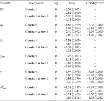
Results of the CIPS test (table 1) show that GDP per capita, total agricultural imports per capita and remittances per capita are I(0) when expressed in their first difference, whereas precipitation (SPI) and financial development (private credit by deposit money banks and other financial institutions as percentage of GDP) variables are stationary variables when expressed in level.
Panel unit root test results

Notes: Series are I(1) under the null hypothesis and p-values are reported in parenthesis.
Using first differenced variables in a VAR model may result in a loss of the long-run information in the presence of a cointegration relationship between the variables. We then use the four panel cointegration tests of Westerlund (Reference Westerlund2007), which have good small-sample properties and high power relative to popular residual-based panel cointegration tests such as the Pedroni test (2004). Furthermore, bootstrap p-values are computed making inference possible under CD.Footnote 9
The G t and G a statistics test the null hypothesis of no cointegration for all cross-sectional units against the alternative that there is cointegration for at least one cross-sectional unit (H 0: ρ i = 0 for all i vs. H 0: ρ i = 0 for at least one i). The P t and P a statistics pool information over all the cross-sectional units to test the null of no cointegration for all cross-sectional units against the alternative of cointegration for all cross-sectional units (i.e. H 0: ρ i = 0 vs. H 0: ρ i = ρ< 0 for all i).Footnote 10
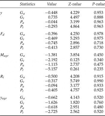
For small samples like ours, Westerlund (Reference Westerlund2007) warns that the results of the tests may be sensitive to the specific choice of lag and lead lengths. Hence, to avoid over-parametrization and the resulting lack of sufficient degrees of freedom, we hold the short-run dynamics by setting up one lag and one lead length (i.e., p i = p = 1) in the panel cointegration test model. The lag order choice is also confirmed by the AIC criterion. Pooled and panel statistics, reported in table 2, indicate no rejection of the null hypothesis that the series are not cointegrated.
Panel cointegration test results

Notes: Each error-correction model includes a constant and no trend under the null hypothesis of no cointegration. Robust critical values are obtained through bootstrapping with 800 replications.
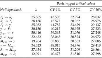
The panel causality test proposed by Emirmahmutoglu and Kose (Reference Emirmahmutoglu and Kose2011) is based on the meta-analysis of Fisher (Reference Fisher1932)Footnote 11 and has several advantages. First, it allows taking into account heterogeneities in the cross-sectional units. A Granger causality test for each unit is calculated with different lag orders (the maximum lag order is set to two lags) based on the AIC criterion. The panel Fisher test statistic (λ) is obtained by combining the p-values corresponding to the Wald statistic for each cross-sectional unit. Secondly, the test allows for cross-sectional dependency. In the case of cross-section dependency in the panel, a bootstrap method is applied to generate the empirical distributions of the Fisher test. The bootstrap distribution of the Fisher test statistics is derived from 5,000 replications and bootstrap critical values are obtained at the 1 per cent, 5 per cent and 10 per cent levels.
Results in table 3 confirm that remittances inflows may have positive or negative effects on the domestic credit provided by the banking sector which, in turn, may contribute to GDP growth. By positioning remittances before financial sector development and GDP variables in the PCHVAR model, we address the potential immediate and lagged spillover effects of remittances on domestic production capacities. Furthermore, Granger causality test results in table 3 show that agricultural imports are Granger-caused by remittances and GDP variables. Agricultural imports are then considered as the most endogenous variable in the system. They are contemporaneously affected by remittances, financial sector development and GDP. Thus the five variables of the system are ordered as follows:
 $$Y_{it}\colon \left[R_i\semicolon \; F_d\semicolon \; y_{agr}\semicolon \; y\semicolon \; M_{agr}\right]$$
Granger causality test results

5. Empirical results
We determine the effects of drought severity and remittances shocks on the set of the considered macroeconomic variables by estimating the PCHVAR model given by equation (6). We compute OIRFs giving the sth-period response when the system is shocked by a one-standard deviation shock, and we also perform a standard variance decomposition exercise (FEDV) for the variables included in the PCHVAR model. Since the model is estimated in logs, the OIRFs show the log deviations of variables with respect to their baseline level, so they can be interpreted as percentage changes.
Results from the estimated PCHVAR model show the various potential impacts of remittances. On the supply side, agents receiving remittances may be pushed to move away from their main activity or to diversify their agricultural production. On the demand side, they can spend remittances to maintain a minimum level of consumption during precipitation shocks and drought periods (Yang and Choi, Reference Yang and Choi2005; Quisumbing et al., Reference Quisumbing, McNiven and Godquin2008). The macroeconomic consequences of such behaviors remain undetermined. Remittances may well promote growth, if they are used to purchase domestically produced goods and services (Glytsos, Reference Glytsos1993), but such consumption smoothing behaviors may also induce an increase in imports, including imports of essential goods (Jovi
 ić and Mitrović, Reference Jovic̃ić and Mitrović2006).
However, macroeconomic impacts exerted by remittances may also be influenced by precipitation shocks, which have direct consequences on agricultural production capacities. In other words, remittances may exert spillover effects on growth during normal periods but may have a pernicious macroeconomic impact when shocks occur. Our findings confirm this conjecture by evidencing that the macroeconomic impact of remittances in West Africa is highly sensitive to drought conditions. Indeed, results from OIRFs and FEDV show that a positive shock in remittances has various macroeconomic effects depending on the level of the six-month Standardized Precipitation Index.
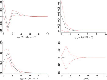
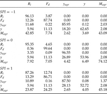
Remittances exert no spillover effects in the countries studied here since they only explain 5.94 per cent of the GDP variance (table 4). This low contribution of remittances inflows to innovations in GDP remains constant for all values taken by the conditioning variable (i.e., the Standardized Precipitation Index). Impulse response functions indicate that a one standard deviation positive shock on remittances has no effect on the real GDP per capita, whatever the weather conditions (figure 1). On the contrary, responses of agricultural value added to remittances positive shocks vary greatly according to the Standardized Precipitation Index (figure 1). Indeed, a one standard deviation positive shock on remittances results in an increase in agriculture value added by 0.98 per cent and in a decline by −0.83 per cent in case of abnormal wet conditions (SPI = 1) and moderate droughts (SPI = −1) respectively, one year after the shock. By contrast, the response of agricultural value added to a positive shock on remittances is found to be non-significant for median values of the Standardized Precipitation Index (SPI = 0).
Agricultural value added and GDP responses to a shock on remittances

Forecast error decomposition variance

Notes: The columns of the table show the fraction of the 10-year ahead forecast error that can be explained by all considered variables in the PCHVAR model. The variance of the 10-year ahead forecast error is almost identical to the unconditional variance of variables. So, figures show the fraction of the total variance of variables that can be accounted by each type of shock.
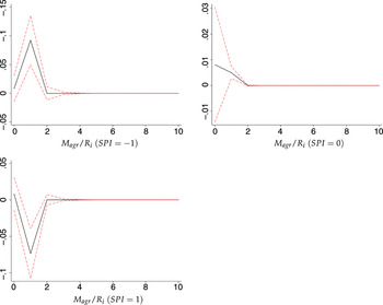
Our results also confirm that remittances inflows may spur agricultural imports especially for low SPI values. The dynamic response of agricultural imports to a shock on remittances is depicted in figure 2. In case of abnormal wet conditions (SPI = 1), impulse response functions show that a positive shock on remittances has a negative impact of −7.35 per cent on agricultural imports one year after the shock. For median values of the SPI (SPI = 0), a one standard deviation positive shock on remittances results in a non-significant response of agricultural imports. Conversely, the effect of such a shock is positive and significant for values of the SPI lower than −0.4. Thus, in case of moderate droughts (SPI = −1) a positive shock on remittances leads to an increase in agricultural imports of 9.23 per cent one year after the shock, gradually returning to normal levels the following year as the initial shock of remittances is diluted. This increase in agricultural imports appears to be a response to the decline in agricultural supply after a rainfall shock, a decline which is not entirely compensated by the rise following remittances inflows.
Agricultural imports responses to a shock on remittances

Analysis of the FEDVs in table 4 corroborates those results. Indeed, remittances only explain a low percentage of the fraction of the variance of agricultural imports in countries characterized by normal SPI values (7.92 percent for SPI = 0). This contribution increases as the Standardized Precipitation Index (SPI) deviates from its baseline. Remittances explain 42.95 per cent and 23.87 per cent of the fraction of the variance of agricultural imports in case of moderate droughts (SPI = −1) and abnormal humid conditions (SPI = 1), respectively.
Thus, our results bring some evidence that import responses to remittances shocks can be interpreted as part of the income strategies of intertemporal smoothing in a context of agricultural supply constraints. In case of adverse weather conditions, the negative response of the agricultural value added to a positive shock in remittances supports previous empirical studies: it shows that remittances inflows may generate moral hazard and then have a negative effect on economic growth (Chami et al., Reference Chami, Fullenkamp and Jahjah2003; Azam and Gubert, Reference Azam and Gubert2005).
A key question is whether remittances have an impact on the financial development of our sampled countries. We find a significant link between remittances and financial development but this link appears to be non-linear, depending also on weather conditions. After controlling for climate shocks, our results are contrary to the view of a positive impact of remittances on financial development in sub-Saharan countries (Gupta et al., Reference Gupta, Pattillo and Wagh2009; Aggarwal et al., Reference Aggarwal, Demirgüç-Kunt and Pería2011). Indeed, we find that adverse weather conditions act as a constraint on the complementarity link between remittances and financial development. Therefore, in West Africa and especially in rural areas characterized by low financial institutions, poorer and most exposed households may prefer to rely on informal services when they face adverse weather events because of high transaction costs in formal financial services, and particularly in credit.
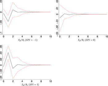
FEDVs show that shocks on remittances account for a large share in the variance of the financial development indicator for extreme values of the standard precipitation index. This contribution in the variance of the financial development indicator increases from 0.36 per cent when the SPI is equal to 0 to 12.26 per cent when SPI = −1 and to 13.29 per cent when SPI = 1. Results from OIRFs in figure 3 indicate that a positive shock on remittances leads to an increase in financial development (4.01 per cent) the year following the shock in case of abnormal humid conditions (SPI = 1) and to a decrease (−4.30 per cent) in case of moderate droughts (SPI = −1).
Financial sector development responses to a shock on remittances

GDP response to a shock on financial sector development

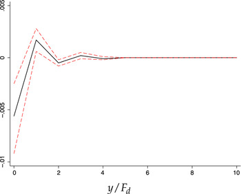
Furthermore, our results also show that GDP per capita responds negatively to positive shocks on financial development. According to FEDVs, the index of financial development contributes to 11.13 per cent in the variance of GDP and OIRFs indicate that a one standard deviation positive shock on private credit to GDP ratio results in an immediate 0.5 per cent decrease in GDP per capita. This response remains negative and significant for every value of the SPI. This confirms previous results showing that the relationship between financial development and growth can be negative in the case of developing countries where strong fragmentation exists between formal and informal financial sectors (Aryeetey et al., Reference Aryeetey, Steel, Hettige and Nissanke1997). Recent studies have also showed that low level of economic development can limit the efficiency of the financial sector (Méon and Weill, Reference Méon and Weill2010).
6. Conclusion
The aim of this paper was to investigate the consequences of remittances inflows on macroeconomic performance for a sample of West African countries facing climate variability. Accordingly, we have implemented an empirical framework based on the estimation of a PCHVAR model where effects of remittances are conditional to rainfall shocks. Rainfall shocks have been computed based on an Standardized Precipitation Index using time series of precipitation data extracted from the CRU.
Our results show that remittances have a significant impact on the macroeconomic performance of West African economies. Yet this impact is highly sensitive to rainfall shocks in a context of vulnerability to climate stress. In the case of humid conditions, a positive shock on remittances leads to an immediate increase in agricultural value added and to a negative response of agricultural imports the year following the shock. Moreover, remittances are found to have a positive role on financial development.
However, this positive role of the remittances on West African macroeconomic performance is no longer observed for lower values of the Standardized Precipitation Index. Indeed, if remittances help increase the households’ resilience to rainfall shocks by smoothing consumption over time, this process leads to a rise of agricultural imports when countries face adverse weather events. In this case, remittances have a negative impact on agricultural value added and financial development and do not exert any short-term spillover effects on growth. The immediate rise of agricultural imports following the remittances ‘boom’ confirms the possibility that remittances may increase a situation of economic dependence particularly when drought conditions prevail.
Appendix 1: Lag selection and stability test results
PCHVAR stability test

Lag order decision rule

Appendix 2: SPI methodology
Following Edwards and McKee (Reference Edwards and McKee1997), the calculation of SPI is done by fitting each climatological precipitation time series to the gamma probability density function:Footnote 12
 $$g\lpar x\rpar = \displaystyle {1 \over \beta^\alpha \Gamma \lpar \alpha\rpar }x^{\alpha-1} e^{-x/\beta} \quad \hbox{ for } x \gt 0$$
where α is a shape parameter, β is a scale parameter and x is the monthly precipitation amount (α > 0 and β > 0). For α > 0 the gamma function Γ (α) is defined by:
 $$\Gamma \lpar \alpha\rpar = \vint_0^\infty x^{\alpha - 1}e^{-x}dx$$
Computation of the SPI involves fitting a gamma probability density function to a given frequency distribution of precipitation totals for a station. The alpha and beta parameters of the gamma probability density function are estimated for each station, for one or different time scales of interest (1, 2, 3, 6, 12, 24 months) and for each month of the year. The maximum likelihood solutions are used to optimally estimate α and β:
 $$\hat{\alpha} = \displaystyle{1 \over 4A}\left(1 + \sqrt{1+ \displaystyle{4A \over 3}}\right)$$
 $$\hat{\beta} = \displaystyle{\bar{x} \over \hat{\alpha}}$$
where,
 $$A = \ln\lpar \bar{x}\rpar - \displaystyle{\sum \ln\lpar x\rpar \over n}$$
with n the number of precipitation observations. Integrating the probability density function with respect to x and attaching α and β parameters yields the cumulative probability distribution function G(x):
 $$G\lpar x\rpar = \vint^x_0 g\lpar x\rpar dx = \displaystyle{1 \over \hat{\beta}^{\hat{\alpha}}\Gamma\lpar \hat{\alpha}\rpar } \vint^x_0 x^{\hat{\alpha} - 1}e^{-x/\hat{\beta}}dx$$
Substituting t for
 $-\displaystyle{x \over \hat{\beta}}$
yields the incomplete gamma function:
 $$G\lpar x\rpar = \displaystyle{1 \over \Gamma\lpar \hat{\alpha}\rpar }\vint^x_0 t^{\hat{\alpha} - 1}e^{-t}dt$$
Since the gamma function is undefined for x = 0 and a precipitation distribution may contain zeros, the cumulative probability becomes:
 $$H\lpar x\rpar = q + \lpar 1 - q\rpar \ G\lpar x\rpar$$
where q = P(x = 0) is the probability of zero (null) monthly precipitation. The cumulative probability distribution H(x) is then transformed into the standard normal random variable Z to yield the SPI (Edwards and McKee, Reference Edwards and McKee1997).
 $$Z = SPI = -\left(t - \displaystyle{c_0 + c_1t + c_2t^2 \over 1 + d_1t + d_2t^2 + d_3t^3}\right)\quad \hbox{ for } 0 \lt H\lpar x\rpar \leq 0.5$$
 $$Z = SPI = +\left(t - \displaystyle{c_0 + c_1t + c_2t^2 \over 1 + d_1t + d_2t^2 + d_3t^3}\right)\quad \hbox{ for } 0.5 \lt H\lpar x\rpar \lt 1.0$$
where,
 $$t = \sqrt{\ln \left(\displaystyle {1 \over \lpar H\lpar x\rpar \rpar ^2}\right)} \quad \hbox{for } 0 < H\lpar x\rpar \leq 0.5$$
 $$t = \sqrt{\ln \left(\displaystyle{1 \over 1 - \lpar H\lpar x\rpar \rpar ^2}\right)} \quad \hbox{for } 0.5 < H\lpar x\rpar < 1.0$$
 $$\matrix {c_0 = 2.5155 \hfill & c_1 = 0.8028 \hfill & c_2 = 0.0103 \cr d_1 = 1.4327 \hfill & d_2 = 0.1892 \hfill & d_3 = 0.0013}$$
For the purposes of this paper studying large areas (countries), SPI is applied equally to wet and dry areas characterized by different types of climate. We calculate SPI using the monthly amount of precipitation (in mm) between 1960 and 2010 for multiple precipitation grid points on a six-month time resolution basis using data from the CRU. We then use the SPI averages at the national scale as the conditioning variable in the PCHVAR model in equation (6).
Appendix 3: Pesaran Cross-Section Dependence test (2004)
Pesaran CD test results