1. Introduction
The Chicago Board Options Exchange (CBOE) introduced the first volatility index, the VXO, in 1993 to measure the market's expectation of a hypothetical 30-calendar-day forward-looking volatility implied by at-the-money S&P 100 index (OEX) options. In September 2003, the CBOE switched into a new methodology to create a redefined volatility index, the VIX, which is calculated based on the weighted prices of a portfolio of 30-calendar-day out-of-the-money S&P 500 index (SPX) calls and puts over a wide range of strike prices. Shortly after the introduction of the new VIX, in March 2004, the CBOE Futures Exchange first launched VIX futures contracts on the VIX index, and in February 2006, VIX options were introduced. The VIX has gained widespread popularity and became the factor benchmark for stock market volatility. It is colloquially referred to as the fear index. Its popularity is to some extent due to the fact that VIX movements are negatively correlated with movements in stock returns, the most plausible explanation being that investors trade SPX options to buy protection during periods of market turmoil, which increases the value of the VIX. Thus, it is vital for researchers to investigate the VIX and its derivatives in relation to the stock market.
With the rapidly increasing popularity of VIX derivatives, deriving appropriate pricing models for VIX derivatives has attracted considerable attention. In recent decades, a growing body of literature has documented the presence of jumps in stock returns and in return volatilities (see, e.g., [Reference Duffie, Pan and Singleton13]). Importantly, incorporating return jumps and variance jumps into the pricing model can further improve pricing of VIX futures and options (see, e.g., [Reference Psychoyios, Dotsis and Markellos27,Reference Sepp29,Reference Sepp30,Reference Zhu and Lian32]). Psychoyios et al. [Reference Psychoyios, Dotsis and Markellos27] develops analytical valuation models for VIX futures and options based on a stochastic volatility with jumps (SVJ) model. Sepp [Reference Sepp29,Reference Sepp30] shows how to apply the SVJ model to the pricing and hedging of VIX futures and options. Lin [Reference Lin22] provides a convexity adjustment approximation for the value of VIX futures by developing a diverse stochastic volatility with a contemporaneous jumps (SVCJ) model.
Lian and Zhu [Reference Lian and Zhu21] presents an analytical exact solution for the VIX futures and options prices obtained via a single integral under the SVCJ model. Furthermore, Bardgett et al. [Reference Bardgett, Gourier and Leippold4] extends the SVCJ model by dividing jumps into positive and negative and derives the pricing formula of VIX options. However, recently, the literature provides clear empirical evidence for the presence of both contemporaneous jumps (CJs) and independent jumps (IJs) in the SPX and VIXFootnote 1 (see, e.g., [Reference Bandi and Reno3,Reference Chen and Ye9,Reference Da Fonseca and Ignatieva11]). Note that the SVCIJ model can capture both CJs and IJs. To the best of our knowledge, an effort to simultaneously consider CJs and IJs has never been pursued in the context of pricing volatility derivatives. In addition, the Poisson arrival intensity of the above-mentioned jump models typically specifies jumps to arrive with constant intensity. This assumption poses problems in explaining the tendency of large movements to cluster over time, and directly, it does not take into account the high-volatility effect or clustered jumps (see, e.g., [Reference Aït-Sahalia, Cacho-Diaz and Laeven1,Reference Bates6]). Hence, the Poisson jump-diffusion model with constant intensity is not ideal for describing the state-dependent jump intensities or clustered jumps observed in financial markets.
Motivated by the above discussions, in this paper, we intended to provide a general stochastic volatility model with both contemporaneous and independent arrival of jumps in a time-varying jump intensity framework, and study the VIX option pricing problems. The proposed model stems from Bandi and Reno [Reference Bandi and Reno3], in which they extend the SVCJ model to a general case, that is, a stochastic volatility model with contemporaneous and independent jumps (SVCIJ). We further extend this model to a framework with time-varying jump intensities. Specifically, the time-varying intensities considered in this paper can be divided into two main categories: (1) The jump intensity depends on the volatility (known as state-dependent arrival intensity), and in particular, the jump intensity is a linear function of the spot variance (see, e.g., [Reference Bates6,Reference Duffie, Pan and Singleton13,Reference Eraker14]). The SVCIJ model with state-dependent jump intensity is labeled “SVCIJ-I”. In this case, the SVCIJ-I model allows jumps to arrive more frequency in high-volatility regimes. In fact, Bates [Reference Bates6] shows that the jump intensity can potentially be time-varying rather than constant, and a state-dependentFootnote 2 jump intensity can help explain the cross-section of stock index option prices.
Lin [Reference Lin22] and Cheng et al. [Reference Cheng, Ibraimi, Leippold and Zhang10] derives closed-form solutions obtained via an integral to the VIX futures and options prices under the SVCJ model with state-dependent intensity, and they show that volatility-dependent intensity and volatility jumps are important for pricing VIX derivatives. (2) The Poisson jump-diffusion models allow for clustered jumps (Hawkes-type propagation), and specifically, a single jump increases the probability of future jumps occurring (see, e.g., [Reference Aït-Sahalia, Cacho-Diaz and Laeven1,Reference Luo, Zhang and Zhang23]). The SVCIJ model that uses Hawkes intensity is labeled “SVCIJ-H”. In this case, the SVCIJ-H model is suitable for addressing the clustering of events because the occurrence of an event can influence the intensity of future events. In the literature, Jing et al. [Reference Jing, Li and Ma19] provides pricing models for VIX options based on an SVJ model that allows for clustering in the VIX, and they provide clear evidence of jump clustering when pricing VIX options, which support self-exciting jump models.
Our study evaluates VIX futures and options using two general models, that is, SVCIJ-I and SVCIJ-H models. The resulting pricing formula for the VIX derivatives based on the proposed models takes the analytical form of one-dimensional Fourier integrals. Notably, the characteristic function based on the SVCIJ model is in closed-form, while those of the characteristic function based on the SVCIJ-I and SVCIJ-H models take numerical form. In detail, we derive the characteristic function of VIX squared under the proposed models, as well as the linear function VIX squared of spot variance and stochastic intensities. Notably, affine structures allow for pricing via Laplace transform methods because the characteristic functions of spot variance and time-varying jump intensity can be efficiently—and in some cases analytically—computed as solutions of generalized Riccati equations. Then, using the integral transform and the characteristic function of VIX squared, we derive the pricing formulas for VIX futures and options. In addition, we study the effects of a flexible jump on probability density of volatility and prices of VIX futures and options by deriving a characteristic function based on these calibrated jump-diffusion models. We seek to understand some properties of VIX implied volatility patterns and demonstrate that the flexible jump structures have a profound impact on the pricing of volatility derivatives. In addition, to illustrate the performance of the proposed models, empirical studies are conducted in which we compare the in- and out-of-sample results of VIX option pricing among alternative models.
This study contributes to the existing literature in several ways:
(i) We propose an SVCIJ-I model and an SVCIJ-H model. The proposed models are very general, of which models including SV, SVJ, SVCJ, SVCI-I and SVCJ-H models can be considered special cases. Moreover, according to the empirical results of previous studies, it is more plausible that the jump structure of the VIX contains both CJs and IJs when jointly calibrated to SPX and VIX data.
(ii) We present analytical formulas for VIX futures and options prices up to a one-dimensional integral based on the proposed models, which take the state-dependent jump intensity and jump clustering into account for pricing. In addition, we derive closed-form formulas for the characteristic function, obtained via a numerical method for the SVCIJ-I and SVCIJ-H models and via closed form for the SVCIJ model.
(iii) In the sensitivity analysis, we demonstrate that CJs have a more significant impact on VIX option prices than IJs. In addition, the price of the VIX option is sensitive to a large dependent coefficient, which means the stochastic jump intensity may not negligible, especially during a financial crisis. Moreover, we find that the Hawkes-type propagation is more sensitive to the VIX option price in the long run than in the short run.
(iv) Unlike equity options, VIX options display a downward-sloping term structure: longer maturity VIX options have lower implied volatility than short maturity options. This persuasive feature persists irrespective of strikes and other conditions (i.e., jump-related parameters) and is very pronounced. As we demonstrate, the flexible jump structure contributes to varying degrees to implied volatility. In the low strike case, the time-varying jump intensity has little effect on implied volatility. The jump structures of CJs and IJs advocated in this paper have distinct and important effects. In the future study of volatility derivatives, CJs and IJs should be considered simultaneously.
(v) The empirical results provide evidence that the SVCIJ-I and SVCIJ-H models significantly outperforms other alternative models in our in- and out-of-sample dates.
This paper is organized as follows. In Section 2, we describe the general jump-diffusion model that we consider in the study and illustrate the probability density of volatility. Section 3 presents our pricing formulas for VIX futures and options prices based on the proposed models. Section 4 provides some numerical verification to examine the correctness of our formulas and investigate the impact of incorporating a flexible jump structure for VIX futures and options prices, and conduct the empirical studies of the model comparisons. Section 5 offers our conclusions. Proofs and some technical details are deferred to the Appendix.
2. The model and volatility distribution
2.1. Model formulation
Inspired by recent research on jump activity,Footnote 3 we consider a stochastic volatility model with both CJs and IJs in a time-varying jump intensity framework. The following dynamics are proposed to model the S&P 500 index,  $S_t$, under the risk-neutral probability measure
 $\mathbb {Q}$:
 \begin{equation} \left\{\begin{aligned} \dfrac{\mathrm{d}S_t}{S_t} & = (r-q-\bar{\zeta}\lambda^{C}_t-\zeta\lambda^{S}_t)\,\mathrm{d}t +\sqrt{V_t}\,\mathrm{d}W^{S}_t + (e^{\bar{J}_S}-1)\,\mathrm{d}N^{C}_t +(e^{J_S}-1)\,\mathrm{d}N^{S}_t,\\ \mathrm{d}V_t & = \kappa(\theta-V_t)\,\mathrm{d}t + \sigma_V\sqrt{V_t}\,\mathrm{d}W^{V}_t + \bar{J}_V\,\mathrm{d}N^{C}_t +J_V\,\mathrm{d}N^{V}_t, \end{aligned} \right. \end{equation}
where  $r$ is the risk-free rate and
 $q$ is the dividend.
 $W^{S}_t$ and
 $W^{V}_t$ are correlated Brownian motions with
 $\mathrm {d}W^{S}_t\,\mathrm {d}W^{V}_t=\rho \,\mathrm {d}t$.
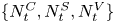 $\{N^{C}_t,N^{S}_t,N^{V}_t\}$ is an independent trivariate Poisson processes with time-varying rate
 $\lambda ^{C}_t$,
 $\lambda ^{S}_t$ and
 $\lambda ^{V}_t$, respectively. The jumps
 $\bar {J}_S$ and
 $\bar {J}_V$ occur simultaneously in the asset price and volatility and are driven by
 $N^{C}_t$. The independent price jump
 $J_S$ and volatility jump
 $J_V$ are driven by
 $N^{S}_t$ and
 $N^{V}_t$, respectively. The jump sizes are assumed to have the following distributions:
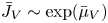 $\bar {J}_V\sim \exp (\bar {\mu }_V)$ with mean
 $\bar {\mu }_V$,
 $\bar {J}_S\,|\,\bar {J}_V \sim N(\bar {\mu }_S+\rho _J\bar {J}_V,\bar {\sigma }_S^{2})$. In addition,
 $\bar {\zeta } \triangleq \mathbb {E}^{\mathbb {Q}}(e^{\bar {J}_S}-1) = e^{\bar {\mu }_S+{\bar {\sigma }_S^{2}}/{2}}/(1-\rho _J\bar {\mu }_V)-1$ and
 $\zeta \triangleq \mathbb {E}^{\mathbb {Q}}(e^{J_S}-1)=e^{\mu _S+{\sigma _S^{2}}/{2}}-1$.
Since the time-varying jump intensity is very popular in recent studies, for example, Bates [Reference Bates7] and Aït-Sahalia et al. [Reference Aït-Sahalia, Cacho-Diaz and Laeven1] report that more jumps occur during more volatile periods, we consider three cases as follows. (1) We first consider the stochastic volatility model with both CJs and IJs in Bandi and Reno [Reference Bandi and Reno3] and Chen and Ye [Reference Chen and Ye9], that is,  $\lambda ^{i}_t=\lambda ^{i}$ is constant for
 $i\in \{C,S,V\}$. (2) The jump intensity is a linear function (e.g., [Reference Bardgett, Gourier and Leippold4,Reference Cheng, Ibraimi, Leippold and Zhang10]) of the instantaneous variance, and in this case, we name the model “SVCIJ-I” (note that the SVCIJ model is a special case of the SVCIJ-I model, where the dependent coefficient
 $\lambda ^{2,C}=\lambda ^{2,S}=\lambda ^{2,V}=0$). (3) The jump intensity ramps up in response to the occurrences of jumps, making further jumps more likely to follow (called “jump propagation”, see, e.g., [Reference Aït-Sahalia, Cacho-Diaz and Laeven1]), and in this case, we denote the model “SVCIJ-H”. A summary of the model specifications is given in Table 1. Our models embrace most of the important derivative pricing models in the literature (such as SVJ, SVIJ, SVCJ and SVCJ-H, i.e., [Reference Aït-Sahalia, Cacho-Diaz and Laeven1,Reference Bates5,Reference Eraker14,Reference Pan24]).
Summary of jump intensities.

Note.  $J_{\lambda }^{i}\sim {\rm Exp}(\mu _{\lambda }^{i})$ with mean
 $\mu _{\lambda }^{i}$,
 $i\in \{C,S,V\}$.
The VIX is primarily related to spot volatility, and we are particularly interested in the effect of the flexible jump structure on spot volatility. In the next section, we study the distributional properties of volatility with respect to CJs and IJs.
2.2. Volatility distribution and jumps
To study how jumps affect volatility, we illustrate the probability density of volatility with CJs and IJs. The probability density function of volatility  $\sqrt {V_T}$ can be obtained through Monte Carlo simulation with 500,000 sample paths. Then, we plot the probability density function of volatility at time
 $T$.
Figure 1 shows how the CJs and IJs of volatility pushes the distribution toward the equilibrium mean level. When the volatility process is examined separately, the CJs should yield the same effect strength as the independent jump. When the jump intensity increases, the volatility of volatility seems to be invariant and the shape of the distribution of volatility tends to be stable.
Probability density function of volatility over a 1-year horizon with different jump intensities, based on the SVCIJ model. The parameter values are shown in Table 2; we simulate 500,000 sample paths of data with length of time  $T$.

Summary of parameter settings.

Note. The superscript  $i\in \{C,S,V\}$.
Naturally, the impact of contemporaneous and independent jumps on volatility cannot be ignored. Jumps in volatility can clearly improve understandings of the dynamics of spot volatility. In addition, Psychoyios et al. [Reference Psychoyios, Dotsis and Markellos27] argues that incorrectly omitting jumps may cause considerable problems in VIX futures and option pricing. Cheng et al. [Reference Cheng, Ibraimi, Leippold and Zhang10] argues that by accounting for return jumps and volatility jumps, the stochastic volatility model can further improve the performance of VIX option pricing formulas. In the next section, we derive formulas for VIX futures and option pricing.
3. The pricing problem
In this section, we turn to the analytical formulas for VIX futures and options (European call options) in the proposed frameworks. The definition of the price of VIX futures at an initial time to maturity  $T$ is given by
 \begin{equation} F(T) = \mathbb{E}_0[\text{VIX}_T]=\int_0^{\infty} xf_{\text{VIX}_T}(x)\, \mathrm{d} x. \end{equation}
The price of the European VIX call option at an initial time to maturity  $T$ and strike
 $K$ is given by
 \begin{equation} C(T,K) = e^{{-}rT} \mathbb{E}_0[(\text{VIX}_T-K)^{+}]=e^{{-}rT} \int_0^{\infty} (x-K)^{+}f_{\text{VIX}_T}(x)\, \mathrm{d} x. \end{equation}
Here,  $f_{\text {VIX}_T}(x)$ is the conditional probability density function of
 $\text {VIX}_T$, and
 $\mathbb {E}_t(\cdotp )$ is conditional on filtration
 $\mathcal {F}_t$ at the current time t. In the sequel, we suppress the superscript and subscript in the expectation operator for notational convenience. We have presented the definitions of prices of options and futures for the VIX, so the question arises, how do we calculate its prices? To address the pricing in the VIX expression, we apply the flexible integral transformation to the formula for futures and options, and they become terse integrals involving the characteristic function
 $\text {VIX}_T^{2}$. Notably, these integral transformations can be expressed as
 \begin{align} \mathbb{E}[\sqrt{x}]& =\frac{1}{2\sqrt{\pi}}\int_0^{\infty} \frac{1-\mathbb{E}(e^{{-}sx})}{s^{3/2}} \mathrm{d}s, \end{align}
 \begin{align} \mathbb{E}[(\sqrt{x}-K)^{+}]& =\frac{1}{2\sqrt{\pi}}\int_0^{\infty} \operatorname{Re}\left[\frac{1-\text{erf}(K\sqrt{\phi})}{\phi^{3/2}}\mathbb{E}(e^{\phi x})\right]\mathrm{d}\phi_I, \end{align}
where the  $s\in \mathcal {R}^{+}$ is a real number,
 $\phi =\phi _R+\phi _Ii$ is a complex number with
 $\phi _R\in \mathcal {R}^{+}$ and
 $\phi _I\in \mathcal {R}$, and erf
 $(Z)$ is a complex error function (see Eq. (14)). A real part of
 $\phi$ greater than zero due to the integral in Eq. (5) exists if and only if
 $\operatorname {Re}(\phi )>0$. The first equation is a mathematical result obtained using Fubini's theorem (proposed by [Reference Schürger, Sandmann and Schönbucher28]), and the second equation is an integral transform using the Parseval identity (proposed by [Reference Lewis20,Reference Poularikas26]). Then, the characteristic functions are the pivotal requirements, which are given by the following section.
3.1. Characteristic function
In this subsection, we present the conditional characteristic functions of  $V_T$ and
 $(\lambda _T^{C},\lambda _T^{S},\lambda ^{V}_T)$ under the risk-neutral measure. The characteristic function
 $\mathcal {L}:\mathbb {C}^{1}\rightarrow \mathbb {C}^{1}$ of some process
 $X_T$ is defined as
 $$\mathcal{L}(\phi;T-t,X_t)\triangleq \mathbb{E}_t(e^{\phi X_T}),$$
where  $T\geqslant t$ and
 $\phi \in \mathcal {D}_x$, and
 $\mathcal {D}_x$ denotes the complex domain of
 $\mathcal {L}(\phi ;T-t,X_t)$, that is
 $$\mathcal{D}_x=\{\phi \in \mathbb{C}: \mathbb{E}[\mathbb{E}_t(e^{\phi X_T})]<\infty\}.$$
The advantage of affine models is that their characteristic function has an exponentially affine form (see [Reference Duffie, Pan and Singleton13]), and thus, various transformations can be quasi-analytically calculated by solving a system of ordinary differential equations (ODEs).
Proposition 1 (Characteristic function of  $V_T$ under the SVCIJ-I model)
If the spot variance  $V_t$ follows the dynamics given by Eq. (1) and the intensities are represented as linear functions of
 $V_t$, Duffie et al. [Reference Duffie, Pan and Singleton13] shows that for any
 $\phi \in \mathcal {D}_v$, where
 $\mathcal {D}_v$ denotes the complex domain of
 $\mathcal {L}(\phi ;\tau,V_t)$, the exponentially affine expression below holds:
 \begin{equation} \mathcal{L}(\phi;\tau,V_t)\triangleq \mathbb{E}_t(e^{\phi V_T}) = e^{h_1(\phi,\tau)V_t + h_2(\phi,\tau)}, \end{equation}
where  $\tau =T-t$ and
 $h_1(\phi,\tau )$,
 $h_2(\phi,\tau )$,
 $h_3(\phi,\tau )$ are solutions of the system of ODEs:
 $$\left\{\begin{aligned} \dfrac{\partial}{\partial\tau}h_1(\phi,\tau) & ={-}\kappa h_1(\phi,\tau)+\frac{1}{2}\sigma_V^{2} h_1^{2}(\phi,t)+\lambda^{2,C}\left(\frac{1}{1-\bar{\mu}_Vh_1(\phi,\tau)}-1\right)\\ & \quad +\lambda^{2,V}\left(\frac{1}{1-\mu_Vh_1(\phi,\tau)}-1\right),\\ \dfrac{\partial}{\partial\tau}h_2(\phi,\tau) & = \kappa\theta h_1(\phi,\tau)+\lambda^{1,C}\left(\frac{1}{1-\bar{\mu}_Vh_1(\phi,\tau)}-1\right) +\lambda^{1,V}\left(\frac{1}{1-\mu_Vh_1(\phi,\tau)}-1\right), \end{aligned} \right.$$
with the initial conditions  $h_1(\phi,0)=\phi$,
 $h_2(\phi,0)=0$.
Proof. We prove this in Appendix B.
Notably, the SVCIJ model is a special case of the SVCIJ-I model. When  $\lambda ^{2,C}=\lambda ^{2,S}=\lambda ^{2,V}=0$, the SVCIJ-I model degenerates into the SVCIJ model. Although it is only the fading of the
 $\lambda ^{2,C}$,
 $\lambda ^{2,S}$ and
 $\lambda ^{2,V}$ parameters, the analytical solution exists for the characteristic function under the SVCIJ model.
Corollary 1 (Characteristic function of  $V_T$ under the SVCIJ model)
The conditional characteristic function of the instantaneous variance  $V_T$ is given by the following exponentially affine expression:
 \begin{equation} \mathcal{L}(\phi;\tau,V_t)\triangleq \mathbb{E}_t(e^{\phi V_T}) = e^{h_1(\phi,\tau)V_t + h_2(\phi,\tau)+h_3(\phi,\tau)}, \end{equation}
where  $\tau =T-t$ and
 $h_1(\phi,\tau )$,
 $h_2(\phi,\tau )$,
 $h_3(\phi,\tau )$ are defined as follows:
 $$\left\{ \begin{aligned} h_1(\phi,\tau) & = \frac{2\kappa \phi}{\sigma_V^{2}\phi+(2\kappa-\sigma_V^{2}\phi)e^{\kappa \tau}},\\ h_2(\phi,\tau) & =\frac{-2\kappa \theta}{\sigma_V^{2}}\ln{\left(1+\frac{\sigma_V^{2}\phi}{2\kappa}(e^{-\kappa\tau}-1)\right)},\\ h_3(\phi,\tau) & =\frac{2\lambda_{C}\bar{\mu}_{V}}{2\kappa\bar{\mu}_{V}-\sigma_V^{2}}\ln \left(1+\frac{(\sigma_V^{2}-2 \kappa \bar{\mu}_{V}) \phi}{2 \kappa(1-\bar{\mu}_{V} \phi)}(e^{-\kappa \tau}-1)\right)\\ & \quad +\frac{2 \lambda_{V} \mu_{V}}{2 \kappa \mu_{V}-\sigma_V^{2}} \ln \left(1+\frac{(\sigma_V^{2}-2 \kappa \mu_{V}) \phi}{2 \kappa(1-\mu_{V} \phi)}(e^{-\kappa \tau}-1)\right), \end{aligned} \right.$$
with the initial conditions  $h_1(\phi,0)=\phi$,
 $h_2(\phi,0)=h_3(\phi,0)=0$, with
 $\phi \in \mathcal {D}_v$. In addition, under this model,
 $\phi _R$ satisfies
 $$\phi_R<\min \left(\frac{2\kappa}{\sigma_V^{2}(1-e^{-\kappa\tau})},\frac 1\mu_V,\frac{2\kappa}{\sigma_V^{2}(1-e^{-\kappa\tau})+2\mu_V\kappa e^{-\kappa\tau}},\frac {1}{\bar{\mu}_V},\frac{2\kappa}{\sigma_V^{2}(1-e^{-\kappa\tau})+2\bar{\mu}_V\kappa e^{-\kappa\tau}}\right).$$
Proof. We prove this in Appendix B.
Proposition 2 (Characteristic function of  $(V_T, \lambda ^{C}_T, \lambda ^{S}_T, \lambda ^{V}_T)$ under the SVCIJ-H model)
If the spot variance  $V_t$ follows the dynamics given by Eq. (1) and the intensity satisfies the bottom row of Table 1, then the conditional joint characteristic function of the instantaneous variance and intensities, for any
 $\boldsymbol {\phi }$ that belongs to their complex domain of
 $\mathcal {L}(\boldsymbol {\phi };\tau,V_t,\lambda ^{C}_t,\lambda ^{S}_t,\lambda ^{V}_t)$, is given by the following exponential affine form:
 \begin{align*} \mathcal{L}(\boldsymbol{\phi};\tau,V_t,\lambda^{C}_t,\lambda^{S}_t,\lambda^{V}_t)& \triangleq \mathbb{E}_t(e^{\phi_1 V_T+\phi_2\lambda_T^{C}+\phi_3\lambda_T^{S}+\phi_4\lambda_T^{V}}) \\ & =e^{h_1(\boldsymbol{\phi};\tau)V_t +h_2(\boldsymbol{\phi};\tau)\lambda^{C}_t+h_3(\boldsymbol{\phi};\tau)\lambda^{S}_t +h_4(\boldsymbol{\phi};\tau)\lambda^{V}_t+h_5(\boldsymbol{\phi};\tau)}, \end{align*}
where  $\boldsymbol {\phi }=(\phi _1,\phi _2,\phi _3,\phi _4,\phi _5)$ and
 $h_1(\boldsymbol {\phi },\tau )$,
 $h_2(\boldsymbol {\phi },\tau )$,
 $h_3(\boldsymbol {\phi },\tau )$,
 $h_4(\boldsymbol {\phi },\tau )$,
 $h_5(\boldsymbol {\phi },\tau )$ are solutions of the system of ODEs:
 $$\left\{ \begin{aligned} h_1(\boldsymbol{\phi},\tau) & = \frac{2\kappa \phi_1}{\sigma_V^{2}\phi_1+(2\kappa-\sigma_V^{2}\phi_1)e^{\kappa \tau}},\\ \frac{\partial}{\partial\tau}h_2(\boldsymbol{\phi},\tau) & ={-}\alpha^{C} h_2(\boldsymbol{\phi},\tau) +\frac{1}{1-\bar{\mu}_Vh_1(\boldsymbol{\phi},\tau)}\times\frac{1}{1-\mu_{\lambda}^{C}h_2(\boldsymbol{\phi},\tau)}-1,\\ \frac{\partial}{\partial\tau}h_3(\boldsymbol{\phi},\tau) & ={-}\alpha^{S} h_3(\boldsymbol{\phi},\tau) +\frac{1}{1-\mu_{\lambda}^{S}h_3(\boldsymbol{\phi},\tau)}-1,\\ \frac{\partial}{\partial\tau}h_4(\boldsymbol{\phi},\tau) & ={-}\alpha^{V} h_4(\boldsymbol{\phi},\tau) +\frac{1}{1-\mu_Vh_1(\boldsymbol{\phi},\tau)}\times\frac{1}{1-\mu_{\lambda}^{V}h_4(\boldsymbol{\phi},\tau)}-1,\\ \frac{\partial}{\partial\tau}h_5(\boldsymbol{\phi},\tau) & = \kappa\theta h_1(\boldsymbol{\phi},\tau)+\alpha^{C}\lambda^{C}_{\infty} h_2(\boldsymbol{\phi},\tau) + \alpha^{S}\lambda^{S}_{\infty} h_3(\boldsymbol{\phi},\tau)+ \alpha^{V}\lambda^{V}_{\infty} h_4(\boldsymbol{\phi},\tau), \end{aligned}\right.$$
with the initial conditions  $h_1(\boldsymbol {\phi },0)=\phi _1$,
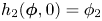 $h_2(\boldsymbol {\phi },0)=\phi _2$,
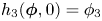 $h_3(\boldsymbol {\phi },0)=\phi _3$,
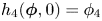 $h_4(\boldsymbol {\phi },0)=\phi _4$,
 $h_5(\boldsymbol {\phi },0)=0$, with
 $\phi _1\sim \phi _4 \in \mathcal {D}_v$.
Proof. We prove this in Appendix B.
Since the above ODEs of  $h_2$,
 $h_3$ and
 $h_4$ of the SVCIJ-I and SVCIJ-H modelsFootnote 4 have no analytical solutions, we use a numerical method, such as the Runge-Kutta algorithm, to solve these ODEs.
3.2. Pricing VIX futures and options
In this section, we present our model framework for pricing VIX futures and options, which is a general case of the previous affine pricing frameworks developed in the previous literature. First, simple affine state dynamics are employed to price the VIX in explicit form in general equilibrium; then, the generalized Laplace payoff transform analysis is conducted and performed to derive a pricing formula for VIX futures and options as a single integral.
The characteristic functions of variance and intensities have been discussed above. To find the characteristic functions of the VIX, a natural idea is to explore VIX squared as a linear function of instantaneous variance and intensities. Fortunately, Duan and Yeh [Reference Duan and Yeh12] provide a linear expression for the relationship between the VIX and variance in a stochastic volatility model. Therefore, we generalize and derive this expression under the SVCIJ-I and SVCIJ-H models. In Lemma 1, we derive the linear relation between the state variable (i.e., the instantaneous variance and time-varying intensity) and the 30-calendar-day VIX under these three models.
Lemma 1 (Linear property of VIX)
The  $\text {VIX}^{2}$ is simply given by an affine transformation of the spot variance and time-varying intensities. The 30-day VIX index is a measure of the risk-neutral expected volatility of the SPX over the next 30 calendar days. Specifically, the calculation formula of VIX squared at a given time
 $t$ is given by
 $$\text{VIX}_t^{2}(\tilde{\tau})=\frac{2}{\tilde{\tau}}\mathbb{E}_t \left[\int_t^{t+\tilde{\tau}}\left(\frac{\mathrm{d}S_u}{S_u}-\mathrm{d}\log S_u\right)\right],$$
where  $\tilde {\tau } = \frac {30}{365}$. To express the VIX as an explicit function in state variables, we follow Duan and Yeh [Reference Duan and Yeh12] in using the affine property of VIX squared. Lemma 1 shows that we can transform VIX squared into state variables
 $V_t$ and
 $\lambda _t$.
(1) For the SVCIJ-I model,
(8)where \begin{equation} \text{VIX}_t^{2} = aV_t+b, \end{equation}
(9)\begin{equation} \left\{ \begin{aligned} a & = \eta(1+2\lambda^{2,C}(\bar{\zeta} - \bar{\mu}_S-\rho_J \bar{\mu}_V)+2\lambda^{2,S}(\zeta - \mu_S)),\\ b & = \frac{B}{A}(1-\eta)+2(\bar{\zeta} - \bar{\mu}_S-\rho_J \bar{\mu}_V)\left(\lambda^{1,C}+\lambda^{2,C}\frac{B}{A}(1-\eta)\right)\\ & \quad + 2(\zeta - \mu_S )\left(\lambda^{1,S}+\lambda^{2,S}\frac{B}{A}(1-\eta)\right). \end{aligned} \right. \end{equation}
Here,
$\bar {\mu }_V\triangleq \mathbb {E}(\bar {J}^{V})$, $\mu _V\triangleq \mathbb {E}(J^{V})$, $\bar {\zeta } \triangleq \mathbb {E}(e^{\bar {J}^{S}}-1)$, $\zeta \triangleq \mathbb {E}(e^{J^{S}}-1)$ and $\eta ={(1-e^{-A\tilde {\tau }})}/{A\tilde {\tau }}$, $A=\kappa -\lambda ^{2,V}\mu _V-\lambda ^{2,C}\bar {\mu }_V$ and $B=\theta \kappa +\lambda ^{1,V}\mu _V+\lambda ^{1,C}\bar {\mu }_V$. For convenience, we abbreviate $\text {VIX}_t(\tilde {\tau })$ as $\text {VIX}_t$. When $\lambda ^{2,C}=\lambda ^{2,S}=\lambda ^{2,V}=0$, this linear relationship can be applied to the SVCIJ model. This linear function can also be expressed as a linear function of $V_t$ and $\lambda _t$ if we substitute $\lambda _t=\lambda ^{1}+\lambda ^{2}V_t$ into the linear result above.(2) For the SVCIJ-H model,
(10)where\begin{equation} \text{VIX}_t^{2} = aV_t+b\lambda_t^{C}+c\lambda_t^{S}+d\lambda_t^{V}+e, \end{equation}
(11)where\begin{equation} \left\{ \begin{aligned} a & = \frac{1-e^{-\kappa\tilde{\tau}}}{\kappa\tilde{\tau}},\\ b & = \frac{\bar{\mu}_V(\varphi(\beta^{C})-a)}{\kappa-\beta^{C}}+2\varphi(\beta^{C})(\bar{\zeta} - \bar{\mu}_S-\rho_J \bar{\mu}_V),\\ c & = 2\varphi(\beta^{S})(\zeta - \mu_S ),\\ d & = \frac{\mu_V(\varphi(\beta^{V})-a)}{\kappa-\beta^{V}},\\ e & = \left(\theta+\frac{\tilde{\lambda}^{C}\bar{\mu}_V + \tilde{\lambda}^{V} \mu_V}{\kappa}\right)(1-a)+2 \tilde{\lambda}^{C} (\bar{\zeta} - \bar{\mu}_S-\rho_J \bar{\mu}_V)(1-\varphi(\beta^{C})) \\ & \quad + 2\tilde{\lambda}^{S} (\zeta - \mu_S )(1-\varphi(\beta^{S}))- \frac{\bar{\mu}_V\tilde{\lambda}^{C}}{\kappa-\beta^{C}}(\varphi(\beta^{C})-a)\\ & \quad-\frac{\mu_V\tilde{\lambda}^{V}}{\kappa-\beta^{V}}(\varphi(\beta^{V})-a), \end{aligned} \right. \end{equation}
$a\sim e$ are constants. Here, $\beta ^{i}=\alpha ^{i}-\mu _{\lambda }^{i}$, $\tilde {\lambda }^{i}=\lambda ^{i}_{\infty }\alpha ^{i}/\beta ^{i}$ and $\varphi (x)={(1-e^{-x\tilde {\tau }})}/{x\tilde {\tau }}$, $i\in \{C,S,V\}$.





Proof. We prove this in Appendix B.
Many studies make use of this linear relationship. Indeed, this linear relationship plays an important role in connecting the latent volatility to the observable VIX in the market. Lemma 1 derives the linear relationship between the  $\text {VIX}_T$ and the two state variables:
 $V_T$ and
 $\lambda _T$. Thus, we can exploit this linear function relationship to obtain the explicit analytical formula for the prices of VIX futures and options under different models. As stated at the beginning of this section, we derive the formulas by the direct integral transformations to calculate the prices of VIX derivatives. See Theorem 1 for the calculation of
 $\text {VIX}$ futuresFootnote 5 and Theorem 2 for the calculation of
 $\text {VIX}$ options.
Theorem 1 (VIX future pricing)
Using the transformation of Eq. (4) and the characteristic function of VIX squared, the price of a VIX future,  $F(T)$, is given by the following formula:
 \begin{equation} F(T)=\mathbb{E}[\text{VIX}_T]=\frac{1}{2\sqrt{\pi}}\int_0^{\infty} \frac{1-\mathbb{E}(e^{{-}s\text{VIX}_T^{2}})}{s^{3/2}}\,\mathrm{d} s. \end{equation}
(1) For the SVCIJ-I model,
where$$\mathbb{E}(e^{{-}s \text{VIX}_T^{2}})=e^{{-}bs}\mathcal{L}({-}as;T,V_t),$$
$s\in \mathbb {R}^{+}$, and the initial value $\text {VIX}^{2}_0=aV_0+b$ and $a, b$ are defined in Eq. (9).(2) For the SVCIJ-H model,
and the initial value$$\mathbb{E}(e^{{-}s \text{VIX}_T^{2}})=e^{{-}es}\mathcal{L}(({-}as,-bs,-cs,-ds);T,V_t,\lambda_t^{C},\lambda^{S}_t,\lambda^{V}_t),$$
$\text {VIX}_0^{2} = aV_t+b\lambda ^{C}_0+c\lambda ^{S}_0+d\lambda _0^{V}+e$ and $a\sim e$ are defined in Eq. (11).


Proof. We prove this in Appendix B.
Notably, the integrals in this paper are integrable, the conditions of the Fubini theorem are satisfied, and the order of integration in Theorems 1 and 2 can be interchanged. Others, such as the Feller condition  $2\kappa \theta >\sigma _V^{2}$, will not be elaborated in the rest of this paper, as the authors have verified its rationality.
Remark 1 The VIX futures prices have a single one-dimensional numerical integration, but for a hypothetical futures contract written on VIX squared (introduced by [Reference Eraker and Wu15]), which has a closed-form expression, since VIX squared is a linear function of  $V_T$ and
 $\lambda _T$, the VIX squared futures prices under the SVCIJ-H model are
 $$F_{\text{VIX}^{2}}(T)=\mathbb{E}(\text{VIX}_t^{2}) = a\mathbb{E}(V_t)+b\mathbb{E}(\lambda_t^{C})+c\mathbb{E}(\lambda_t^{S})+d\mathbb{E}(\lambda_t^{V})+e.$$
A European VIX call renders its holder the right, but not obligation, to obtain the difference between the VIX index at an expiration date  $T$ and a pre-specified strike
 $K$. Compared to an equity option, it is more convenient to directly calculate price of a VIX call without normalization. The no-arbitrage condition implies that the VIX call price is represented by the following theorem.
Theorem 2 (VIX call option pricing)
Using the transformation of Eq. (5) and the characteristic function of VIX squared, the price of a VIX call option,  $C(T,K)$, is given by the following formula:
 \begin{equation} C(T,K) =\mathbb{E}[(\text{VIX}_T-K)^{+}]=\frac{e^{{-}rT}}{2\sqrt{\pi}}\int_0^{\infty} \operatorname{Re}\left[\frac{1-\text{erf}(K\sqrt{\phi})}{\phi^{3/2}}\mathbb{E}(e^{\phi \text{VIX}_T^{2}})\right]\mathrm{d}\phi_I, \end{equation}
where  $\phi =\phi _R + i \phi _I$ is the complex Laplace transform variable with
 $\phi _I\in \mathbb {R}$ and
 $\phi _R>0$ and where the complex error function
 $\text {erf}(Z)$ is defined by
 \begin{equation}\text{erf}(Z) = \frac{2}{\sqrt{\pi}}\int_0^{Z} e^{{-}s^{2}}\,\mathrm{d}s.\end{equation}
(1) For the SVCIJ-I model,
with the initial value$$\mathbb{E}(e^{\phi \text{VIX}_T^{2}})=e^{b\phi}\mathcal{L}(a\phi;T,V_t),$$
$\text {VIX}^{2}_0=aV_0+b$.(2) For the SVCIJ-H model,
with the initial value$$\mathbb{E}(e^{\phi \text{VIX}_T^{2}})=e^{e\phi}\mathcal{L}((a\phi,b\phi,c\phi,d\phi);T,V_t,\lambda_t^{C},\lambda^{S}_t,\lambda^{V}_t),$$
$\text {VIX}_0^{2} = aV_t+b\lambda ^{C}_0+c\lambda ^{S}_0+d\lambda _0^{V}+e$.


Proof. We prove this in Appendix B.
Our formulas are extremely efficient and accurate for calculating the futures and options prices of  $\text {VIX}_T$, regardless of whether the model considers both CJs and IJs or time-varying intensities. We use clever integral transformations, and the formula involves only a single integral and thus exhibits more efficiency. In the next section, we perform some numerical experiments to verify the correctness of our formulas by comparing the results calculated by the Monte Carlo simulation with the results obtained by our formulas.
4. Numerical analysis
To verify the correctness of our formulas, we perform numerical analysis in this subsection for comparison (similar to [Reference An and Li2,Reference Han18,Reference Pasricha and Goel25]). We use Monte Carlo simulations with 200,000 sample paths on a short discrete time grid to approximate the true options and futures. The numerical results are displayed in Tables 3 and 4.
Prices of VIX futures.

Note. Here  $\tau$ is time to maturity (or the tenor of VIX derivatives),
 $F_{\text {MC}}$ are prices of VIX futures calculated by Monte Carlo simulation, and
 $F$ are prices of VIX futures calculated by our formula. We simulate 200,000 sample paths and include 1,000 observations (1 year) in each path.
Prices of VIX call options.

Note. Here  $\tau$ is time to maturity (or the tenor of VIX derivatives),
 $C_{\text {MC}}$ are prices of VIX options calculated by Monte Carlo simulation and
 $C$ are prices of VIX options calculated by our formula. K is the strike price. We simulate 200,000 sample paths and include 1,000 observations (1 year) in each path.
4.1. Monte Carlo simulations
Euler discretization can be used to approximate the path of the variance and intensity processes over a discrete interval; in this case, we choose a discrete time small enough for  $\Delta t=1/1,000$. The discretization of the variance and intensity processes are
 \begin{align*} V_t& =V_{t-1}+\kappa(\theta-V_{t-1})\Delta t+\sigma_V\sqrt{|V_{t-1}|}\sqrt{\Delta t}\epsilon_t+\bar{J}_VN_t^{C}+J_VN^{V}_t,\\ \lambda_t^{i}& =\lambda^{1,i}+\lambda^{2,i}V_t,\quad (\text{SVCIJ-I model}, i\in\{C,V\}),\\ \lambda_t^{i}& =\lambda_{t-1}^{i}+\alpha^{i}(\lambda_{\infty}^{i}-\lambda_{t-1}^{i})\Delta t+J_{\lambda}^{i}N^{i}_t,\quad (\text{SVCIJ-H model},i\in\{C,S,V\}), \end{align*}
where  $\epsilon _t\sim \mathcal {N}(0,1)$,
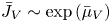 $\bar {J}_V\sim \exp {(\bar {\mu }_V)}$,
 $J_V\sim \exp {(\mu _V)}$,
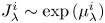 $J^{i}_{\lambda }\sim \exp {(\mu _{\lambda }^{i})}$,
 $N_t^{i}\sim {\rm Bernoulli}(\lambda _{t-1}^{i}\Delta t)$ (
 $\lambda _{t-1}^{i}$ is constant for the SVCIJ model).
With the sample path of variance and intensities (if any), we calculate the sampling VIX path according to  $\text {VIX}_T^{2}=aV_T+b\lambda ^{C}_T+c\lambda ^{S}_T+d\lambda ^{V}_T+e$ or
 $\text {VIX}_T^{2}=aV_T+b$. Then, we obtain the VIX futuresFootnote 6 by
 $({1}/{N})\sum _{i=1}^{N}\text {VIX}_{T,i}$ and VIX options by
 $({1}/{N})\sum _{i=1}^{N}(\text {VIX}_{T,i}-K)^{+}$, where
 $N$ is the number of trajectories and
 $\text {VIX}_{T,i}$ is the value in
 $i$th trajectory at time
 $T$.
To measure the error between the Monte Carlo method and the results calculated by our formulas, we provide two measures: absolute error and relative error, which are defined as follows:
 \begin{align*} \text{absolute error}& =|V-V_{\text{MC}}|,\\ \text{relative error}& =\frac{|V-V_{\text{MC}}|}{V_{\text{MC}}}, \end{align*}
where  $V=F$,
 $C$ represent futures and options, respectively.
In our experiments, we supposed all parameters (see Table 2). In fact, suitable arbitrary parameters have no effect on the accuracy of our formula calculation.
4.2. Accuracy check
Table 3 shows the comparison of VIX futures prices obtained from our formula and Monte Carlo simulations, Table 4 shows the comparison of VIX options prices obtained from our formula and Monte Carlo simulations. The Monte Carlo simulation uses 200,000 sample paths and each path with time steps of 1/1,000. We list the results of the three models for given parameters and find that all three models match perfectly with those obtained from the Monte Carlo simulations.
It is clear that the differences between the results of our futures pricing formula and the Monte Carlo simulation results (the 200,000 Monte Carlo simulated trajectories) are very small, and the relative error range is between 0% and 0.13%. This confirms the accuracy of our futures calculation formula.
The differences between our formula's option prices and the simulation results are small, in the range of 0% to 1.75%. If we regard the Monte Carlo price as the benchmark, then this adequately demonstrates that both our option pricing formula and futures pricing formula are accurate. We have reason, theoretically, to believe that even with different calculation formulas, as long as the given parameters and model are the same, the pricing results are consistent. For the SVCIJ-H model, since the SVCIJ model is a special case of the SVCIJ-I model, to more reliably verify the formula of the SVCIJ-I model, we take  $\lambda ^{2,C}$,
 $\lambda ^{2,S}$ and
 $\lambda ^{2,V}$ to be the large value of 20.
Compared with futures contracts written on commodities and equities, VIX futures are quite unusual. As time to maturity increases substantially, the prices of VIX futures flatten out and become less sensitive to the time to maturity. In the limiting case, VIX futures prices tend toward a constant, this phenomenon of the term structure of VIX futures prices is in line with the observed traded VIX futures prices in the CBOE (see, e.g., [Reference Eraker and Yang16]). This phenomenon is due to volatility's mean-reverting nature, which means that over the long run, volatility tends to revert its long-run average. For the SVCIJ-I model,  $\mathbb {E}(V_T)\stackrel {T\rightarrow \infty }{\longrightarrow }(\theta \kappa +\lambda ^{1,C} \bar {\mu }_V+\lambda ^{1,V}\mu _V)/(\kappa -\lambda ^{2,C}\bar {\mu }_V-\lambda ^{2,V}\mu _V)$ is the long-run mean of variance. For the SVCIJ-H model,
 $\mathbb {E}(V_T)\stackrel {T\rightarrow \infty }{\longrightarrow } (\kappa \theta +\tilde {\lambda }^{C}\bar {\mu }_V+\tilde {\lambda }^{V}\mu _V)/\kappa$ is the long-run mean of variance, and
 $\lim _{T\rightarrow \infty }\mathbb {E}(\lambda ^{i}_T)\stackrel {T\rightarrow \infty }{\longrightarrow }\tilde {\lambda }^{i}$ (
 $i\in \{C,S,V\}$) are the long-run means of intensities. All of these limits above mean that as time-to-maturity increases, prices are becoming less sensitive to initial volatility or jump intensities changes. The existence of these limits confirms that as the time-to-maturity increases, the futures price tends toward a constant.
 \begin{equation} \lim_{T\rightarrow\infty} F(T) =\text{Constant}, \end{equation}
where the constant is a value independent of the VIX. The left panel of Figure 2 illustrates the prices of VIX futures approaching a constant (based on the SVCIJ-H model).
The prices of VIX futures and options over long maturities, based on the SVCIJ-H model.

For this property of volatility, it is natural that the price of its options tends to be close to zero at long maturities. We can also derive this from our formula for options pricing (Eq. (13)), where the integral is bounded, and  $e^{-rT}$ goes to zero as
 $T$ increases.
 \begin{equation} \lim_{T\rightarrow\infty} C(T,K) =0. \end{equation}
The right panel of Figure 2 illustrates the prices of VIX options are approaching a constant. Therefore, at long maturities, the VIX call option will become worthless and less sensitive (which is in line with the results of the models of [Reference Eraker and Yang16,Reference Lian and Zhu21]).
4.3. Sensitivity analysis
To further study the jump structure, we investigate the sensitivity of the VIX options with respect to the parameters of the jump parameters in Figures 3–5. To identify the ceteris paribus effects on the VIX options, we change one or more parameters while holding all remaining parameters fixed. For each parameter set, we plot the 3D diagram of VIX options against time to maturity and the parameters to be studied.
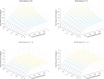
The prices of VIX options ( $K=25$), based on the SVCIJ model.

Naturally, considering the upward jump risk in the model, the call price would increase. Eraker et al. [Reference Eraker, Johannes and Polson17] shows that the SVCJ and SVIJ models exhibit similar behavior, but the SVIJ model is more flexible than the SVCJ model. Therefore, we may also be concerned about how the jump factors affect VIX futures and options in detail under the more general jump-diffusion models. This section examines how jump factors impact VIX derivatives pricing. These prices of VIX derivatives are calculated from our pricing formulas. Figure 3 illustrates the sensitivity of a VIX call option to CJs and IJs in volatility and time to maturity under the SVCIJ model.
Figure 3 illustrates the scenarios for different types of jumps, showing that the call price is affected by various jumps (by setting different jump intensities), especially for CJs. In particular, the top panels of Figure 3 show that the VIX call price is more sensitive to CJs for long-term contracts. These results are in line with the markets because CJs are frequently accompanied by crises and systemic risks, while most IJs occur independently of variance and are relatively accidental. Therefore, from the perspective of the pricing of VIX derivatives, CJs deserve more attention.
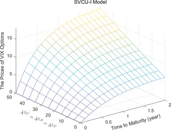
Figure 4 illustrates the scenarios for different  $\lambda ^{2,C}$,
 $\lambda ^{2,S}$ and
 $\lambda ^{2,V}$, showing that the call prices are relatively sensitive to the time-varying intensities, especially for large
 $\lambda ^{2,C}$,
 $\lambda ^{2,S}$ and
 $\lambda ^{2,V}$. Alternatively, by removing the time-varying component of intensities, which is achieved by setting
 $\lambda ^{2,C}=\lambda ^{2,S}=\lambda ^{2,V}=0$, we can obtain the SVCIJ model. In addition, a large
 $\lambda ^{2,C}$,
 $\lambda ^{2,S}$ and
 $\lambda ^{2,V}$ are also associated with higher derivative prices and is more sensitive to time to maturity. Therefore, when the coefficient
 $\lambda ^{2,C}$,
 $\lambda ^{2,S}$ and
 $\lambda ^{2,V}$of the time-varying component of jump intensity may be large, we may not be able to ignore its effect on pricing.
The prices of VIX futures and options ( $K=26$), based on the SVCIJ-I model.

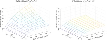
Figure 5 shows the sensitivity of a VIX call price to the impacts of jumps in intensity and time to maturity in the short run and long run (by setting  $\alpha ^{C}$,
 $\alpha ^{S}$ and
 $\alpha ^{V}$ to a large value or small value), which shows that the VIX call prices with
 $\alpha ^{C}=\alpha ^{S} =\alpha ^{V}=2$ (long run) are more sensitive than VIX call prices with
 $\alpha ^{C}=\alpha ^{S}=\alpha ^{V}=15$ (short run). This is because of the significant difference in the mean-reversion speed of intensity. For the SVCIJ-H model, VIX squared is not only related to spot variance but also linearly related to time-varying jump intensities. Thus, intensities can affect VIX squared not only by acting on spot variance but can also directly affect VIX squared.
The prices of VIX options (K=26), based on the SVCIJ-H model.

In summary, although variance jumps in CJs and IJs are both important to the pricing of VIX options, CJs seem to be more important. The time-varying intensity as a linear function of variance seems to be important in pricing VIX derivatives when variance has a large effect on intensity. More important, the mean-reversion of intensity mitigates the value of jumps in intensity. In the case of fast mean-reversion speed, the jumps in intensity seem to have little effect on pricing VIX calls.
4.4. Impact of jumps in implied volatility
To characterize the pricing of VIX call options, we investigate implied volatility. Specifically, we perform numerical tests to investigate the behavior of the implied volatility of VIX options. Recall that the implied volatility  $\sigma _t^{{\rm implied}}$ associated with
 $F(T)$ and
 $C(T,K)$ is defined by inverting the Black and Scholes [Reference Black and Scholes8] formula (see Appendix A for details). Figure 6 shows the implied volatility with the strike price under different maturities and
 $V_0$. Figures 7 and 8 illustrate the implied volatility patterns generated by varying jump parameters. Table 5 reports the implied volatility with respect to the maturity and strike under the SVCIJ model with different jump patterns.
Implied volatility for VIX option in the SVCIJ model. Note. In the left panel, we set varying values of maturity in the SVCIJ model. In the right panel, we set varying values of spot variance  $V_0$ and a fixed maturity at
 $\tau =0.5$ in the SVCIJ model.

Implied volatility for VIX option with maturity  $\tau =0.5$ with respect to the SVCIJ model and SVCIJ-I model. Note. In the left panel, we set varying values of the jump intensity of contemporaneous and volatility-independent jumps in the SVCIJ model. In the right panel, we set varying values of the dependent coefficient in the SVCIJ-I model.

Implied volatility for VIX option with maturity  $\tau =0.5$ in the SVCIJ-H model. Note. In the left panel, we set the mean reversion of both intensities very low (
 $\alpha ^{C}=\alpha ^{S}=\alpha ^{V}=2$, implying long-run intensities) and set varying values of jump size intensities in the SVCIJ-H model. In the right panel, we set the mean reversion of both intensities very high (
 $\alpha ^{C}=\alpha ^{S}=\alpha ^{V}=15$, implying short-run intensities) and set varying values of jump size intensities in the SVCIJ-H model.

Implied volatility for the SVCIJ model.

Note. The table reports implied volatility for VIX options with respect to maturity and strike in the SVCIJ model, as well as the jump intensities of contemporaneous and volatility-independent jumps.  $\tau$ is the maturity, and
 $\lambda ^{C}$ and
 $\lambda ^{V}$ are jump intensities.
There are several noteworthy features of implied volatility.
First, in the SVCIJ model, for a given strike, the implied volatility is greater for short-maturity options (left panel of Figure 6). That is, the term structure of implied volatility is downward sloping irrespective of the level of VIX. To understand why this is, it is crucial to understand that implied volatility, in this case calculated from the Black–Scholes model for pricing an option on VIX futures, assumes that the underlying follows a random walk. If a given process is a random walk, its forecasted variance increases linearly with the forecast horizon. VIX options exhibit a downward-sloping term structure, and therefore, the VIX variance does not increase proportionally with the forecast horizon. Rather, it suggests that the VIX is not a martingale.
Second, the shapes of the implied volatility uniformly form a concave “frown” rather than the usual convex “smile” seen in most equity options, such as SPX options.
Third, low (high) strikes, over some strike range, generally have low (high) implied volatilities, suggesting a positively skewed underlying distribution. Unlike equity options, which exhibit a negative skew in implied volatility, implied volatility in VIX options exhibits positive skew. Notably, accounting for positive jumps in volatility can explain the positive implied volatility skew exhibited by options written on volatility such as CBOE's VIX options. For the SVCIJ-H model, VIX squared would be a linear function of  $V_t$ and
 $\lambda _t$. Similarly, the positive jumps in
 $\lambda _t$ can also be explained by the positive VIX implied volatility skew.
Fourth, the implied volatility values decrease as the initial variance  $V_0$ increases but not significantly.
In the rest of this section, we investigate the sensitivity of the implied volatility of VIX options to the jump-related parameters in the proposed models. To identify the ceteris paribus effects on the implied volatility, we change the specified jump-related parameters while holding all remaining parameters fixed. For each parameter set, we plot the implied volatility curve against the strike.
For the SVCIJ model, Figure 7 shows the implied volatility under different jump structures against the strike. As the figure shows, the CJs and IJs are evident: the structures under CJs and IJs have different implied curves, but for a given jump intensity, the implied volatility is greater for IJs. The implied volatility of IJs is indistinguishable, and the implied volatility curve is very close. However for CJs, there is a significant decreasing trend given increases in  $\lambda ^{V}$ over some strike range. Moreover, the impact of these CJ and IJ jump structures on implied volatility is consistent at different maturity horizons. Table 5 shows the VIX implied volatility surface under different jump structures against strike and maturity. In addition, we know from the previous section on option sensitivity that IJs are not sensitive to option prices, while CJs are considerably more sensitive. This point of view reflects the significance of distinguishing CJs and IJs in our model. During the financial crisis, there were relatively more CJs, while IJs generally predominate (evidence from [Reference Chen and Ye9]). This is reflected by the fact that our stochastic volatility model contains both CJs and IJs.
For the SVCIJ-I model, the left panel of Figure 7 shows the implied volatility against the dependent coefficient  $\lambda ^{2,C}$ and
 $\lambda ^{2,V}$. We observe that the yellow curve is close to the green curve and that the red curve is close to the purple curve, which means that if
 $\lambda ^{2,C}$ and
 $\lambda ^{2,V}$ are of the same value, then the impact on implied volatility is similar. However, note that, in the low strike, the implied volatility on
 $\lambda ^{2,C}$ is smaller, in the high strike, it is greater, relative to implied volatility on
 $\lambda ^{2,V}$ of the same value. In the low strike, the implied volatility in the non-zero dependent coefficient is close to the implied volatility for a zero dependent coefficient. In our SVCIJ-I model, therefore, when a strike is small, the effect of the dependent coefficient on implied volatility is relatively small.
In the previous section, we illustrated the option sensitivity in the long run ( $\alpha ^{C}=\alpha ^{S}=\alpha ^{V}=2$) and short run (
 $\alpha ^{C}=\alpha ^{S}=\alpha ^{V}=15$). We are interested in the implied volatility patterns generated by different mean reversions of jump intensity. Figure 8 shows the result when we condition on high and low mean reversion intensity. We see that the implied volatility curves are almost always increasing with respect to jump size intensity increases, especially under long-run mean reversion. In the short-run case, jump size intensity has no significant effect on implied volatility. However, for a low strike, it does not appear to have much effect on implied volatility. Our model shows that as maturity increases, the futures price also increases and exhibits the concave “frown” pattern. This implies that VIX option-implied volatility is positively correlated with the VIX itself. In the SVCIJ-H model, a fluctuating
 $\lambda _t$ process is important in shaping the positive correlation between implied volatility and the VIX. This can be interpreted to mean that, first, as
 $\lambda _t$ increases, it drives up the VIX because the VIX loads positively on it; second, it also drives up implied volatility and thereby increases the prices of VIX calls. Part of this phenomenon is strikingly similar to the price sensitivity of options discussed previously.
4.5. Empirical studies
In this section, we introduce market data and investigate whether the flexible jump structure improves pricing performance of VIX options. The market data used in this paper include VIX futures, LIBOR and VIX options that provided by the CBOE and OptionMetrics. The sampling dates are June 21, 2017 (Wednesday) as in-sample data for model calibration, and June 22, 2017 (Thursday) as out-of-sample data for evaluating model performance. We filter the option data as follows: (1) we use the mid price (the average of the best bid and best ask) as the market VIX option price; (2) we eliminate any options with zero bid-quote and trading volumes; and (3) we consider only VIX call options because the trading volume of VIX calls is more than puts. Table 6 provides the summary statistics of VIX option data divided into three categories based on moneyness. Here, moneyness is defined as  $m:=\ln (K/F)$ with the strike price of option
 $K$ and corresponding VIX future price
 $F$.
Summary statistics of VIX option data.

Note. The table is divided into three categories based on moneyness (defined as  $m:=\ln (K/F)$ with the strike price of option
 $K$ and corresponding VIX future price
 $F$) on June 21, 2017 (in-sample) and June 22, 2017 (out-of-sample). The reported observation is the number of VIX call option contracts.
For ease of comparison among different models, four typical models are considered: SV model, SVCIJ model and two generalized forms of SVCIJ model by allowing independent return jump to be self-exciting (i.e., SVCIJ-I and SVCIJ-H). Table 7 presents the estimated results by minimizing the mean-square error between market prices and model option prices. The estimated value of  $\lambda ^{2,S}$ is 139.2725 of SVCIJ-I model, which implies that state-depend jump intensity may not be ignored. The estimated value of
 $\alpha ^{S}$ and
 $\mu _{\lambda }^{S}$ of the SVCIJ-H model are 11.2192 and 11.6707, respectively, which implies that Hawkes-type propagation also plays a very important role.
Calibrated model parameters.

Note. The table exhibits the calibration results of VIX option for SV, SVCIJ, SVCIJ-I, and SVCIJ-H modes. The parameters are backed out by minimizing the mean-square error between market and model option prices by using the in-sample data (June 21, 2017).
Next, we compare the performance among different models based on the mean absolute percentage errors (MAPE), which is defined as:
 $$\text{MAPE}=\frac{1}{N_t}\sum_{i=1}^{N_t}\frac{|C_i^{{\rm Model}}-C_i^{{\rm Market}}|}{C_i^{{\rm Market}}},$$
where  $N_t$ is the number of VIX call option contracts on day
 $t$,
 $C_i^{{\rm Market}}$ is the market price of contract
 $i$ and
 $C_i^{{\rm Model}}$ represents the model-implied price of contract
 $i$.
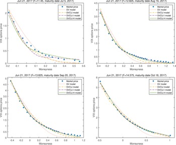
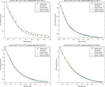
Figure 9 presents a cross-sectional VIX option pricing performance on in-sample data for different maturities and moneyness. It is clear that our proposed models can match market VIX option prices well for the long maturity date and OTM options. Furthermore, the advantage of our models over the benchmark model are most significant for short maturity date and ITM options. Figure 10 shows a cross-sectional VIX option pricing performance on out-of-sample data for different maturities and moneyness and have a similar behavior with in-sample result. Table 8 gives the in-sample and out-of-sample pricing errors of VIX option across different categories of moneyness and maturity, respectively. Clearly, both SVCIJ-I and SVCIJ-H have better performance than other models in all categories. Additionally, we find that the SVCIJ-I and SVCIJ-H have similar performance. Note that the long-term maturity and OTM options show the lowest price errors. Overall, our models provide the best in-sample fitting and out-of-sample prediction across all moneyness and maturities.
In-sample pricing performance of VIX options against moneyness on June 21, 2017. Note. The moneyness is defined as  $\ln (K/F)$ with the strike price of option
 $K$ and corresponding VIX future price
 $F$.

Out-of-sample pricing performance of VIX options against moneyness on June 21, 2017. Note. The moneyness is defined as  $\ln (K/F)$ with the strike price of option
 $K$ and corresponding VIX future price
 $F$.

VIX option pricing errors.

Note. It presents in-sample (June 21, 2017) and out-of-sample (June 22, 2017) option pricing errors for different ranges of moneyness and maturity for the SV, SVCIJ, SVCIJ-I and SVCIJ-H models.
Abbreviations: MAPE, mean absolute percentage errors; m, moneyness; DTM, days to maturity.
5. Conclusion
Motivated by the growing literature on VIX derivatives and their popular introduction in major exchanges, this paper studies the pricing problem for VIX futures and options based on the SVCIJ model with a flexible jump structure. In addition, we study how the jump structure impacts the volatility distribution and VIX derivatives, and carry out the empirical comparison studies of alternative models for the VIX option pricing. This study contributes to the existing literature in several ways. First, the proposed SVCIJ model is a very general model, of which models including the SV, SVJ, SVIJ and SVCJ models can be considered special cases. We present analytical formulas for VIX futures and options prices up to an integral based on the proposed model, which can be considered an extension of the classical Heston model and the jump-diffusion model. Second, we incorporate the volatility-dependent jump intensity and Hawkes intensity into the SVCIJ model and derive the pricing formulas for VIX futures and options prices. Third, having a “fat tail” in the volatility distribution may be caused by incorporating jumps into stochastic volatility model, and contemporaneous jumps have a greater effect on VIX derivative prices than do independent jumps. Fourth, the flexible jump structures contribute to varying degrees to implied volatility. Finally, the in- and out-of-sample results indicate that our proposed models have excellent pricing performance among alternative models. Overall, our models can be used to price a wide range of derivatives, which can be achieved by using the Fourier transform technique, and the stochastic jump intensity may not negligible, especially during a financial crisis.
Acknowledgments
The authors are grateful to Ning Cai (the associate editor) and the anonymous reviewers for helpful guidance and constructive comments. Wuyi Ye's research is supported by the National Natural Science Foundation of China (Grant 71973133 and 71671171).
Appendix A. Black–Scholes implied volatility
We investigate the implied volatility of VIX calls; in contrast to equity options, the underlying asset of a VIX option is not the VIX index itself. Instead, it is a VIX futures contract with same maturity as the VIX option. Thus, we need equate the pricing formula of options on futures in Black and Scholes [Reference Black and Scholes8] with the VIX option price either in the data or obtained from the model and then invert the formula to obtain the implied volatility. Specifically, consider a VIX call with strike  $K$, time to maturity
 $T$ and underlying option price
 $F(T)$. Then, the price of the VIX call should be given by
 $$BS(F(T),K,T,r,\sigma)=e^{{-}rT}[F(T)\cdot N(d_1)-K\cdot N(d_2)],$$
where
 \begin{align*} d_1& =\frac{\ln (F(T)/K)+\sigma^{2}T/2}{\sigma\sqrt{T}},\\ d_2& =d_1-\sigma\sqrt{T}. \end{align*}
Therefore, the model-implied volatility  $\sigma _t^{{\rm implied}}$ should solve
 $$C(T,K)=BS(F(T),K,T,r,\sigma_t^{{\rm implied}}),$$
where  $C(T,K)$ is given by Eq. (13) and
 $r$ is the risk-free rate.
Appendix B. Proofs
Proof of Proposition 1. Proof of Proposition 1.
The conditional characteristic function of  $V_T$ is defined as
 $\mathcal {L}(\phi ;\tau,V_t)\triangleq \mathbb {E}^{\mathbb {Q}}_t(e^{\phi V_T})$. By adopting the temporal variable,
 $\tau =T-t$, it can be deduced from the Feynman-Kac theorem that
 $\mathcal {L}(\phi ;\tau,V_t)$ is governed by the following PIDE:
 \begin{align} 0& ={-}\frac{\partial \mathcal{L}}{\partial \tau} + \kappa(\theta-V_t)\frac{\partial \mathcal{L}}{\partial V_t} +\frac{1}{2}\sigma_V^{2} V_t \frac{\partial^{2} \mathcal{L}}{\partial V_t^{2}}+ \lambda_t^{C} \mathrm{E}_t^{\mathbb{Q}}(\mathcal{L}(\phi;\tau,V_t+\bar{J}^{V})-\mathcal{L}(\phi;\tau,V_t))\nonumber\\ & \quad +\lambda_t^{V} \mathrm{E}_t^{\mathbb{Q}}(\mathcal{L}(\phi;\tau,V_t+J^{V})-\mathcal{L}(\phi;\tau,V_t)), \end{align}
with  $\mathcal {L}(\phi ;0,V_T)=e^{\phi V_T}$. Define
 $X_t=(\ln S_t,V_t)'$,
 $W_t=(W^{S}_t,W_t^{V})'$ and
 $\lambda (X_t)=(\lambda ^{C}_t,\lambda ^{S}_t,\lambda ^{V}_t)'$ and the Markov process
 $X_t$ equivalent to
 $$\mathrm{d}X_t=(\mathcal{M}+\mathcal{K}X_t)\,\mathrm{d}t+\Sigma(X_t)\,\mathrm{d}W_t +\bar{J}\,\mathrm{d}N^{C}_t+J\,\mathrm{d}N_t,$$
where
 \begin{align*} \Sigma(X_t)& =\begin{bmatrix} \sqrt{V_t} & 0\\ 0 & \sigma_V\sqrt{V_t} \end{bmatrix};\quad \bar{J}=\begin{bmatrix} \bar{J^{S}} & 0\\ 0 & \bar{J}^{V} \end{bmatrix};\quad J=\begin{bmatrix} J^{S} & 0\\ 0 & J^{V} \end{bmatrix};\\ \mathrm{d}N_t^{C}& =(\mathrm{d}N_t^{C},\mathrm{d}N_t^{C})';\quad \mathrm{d}N_t=(\mathrm{d}N_t^{S},\mathrm{d}N_t^{V})'. \end{align*}
The affine dependence of  $\mathcal {M}$,
 $\mathcal {K}$,
 $\Sigma (X_t)\Sigma (X_t)'$ and
 $\lambda (X_t)$ are given by
 \begin{align*} \mathcal{M}=(r-q-\bar{\zeta}\lambda^{C}_t-\zeta\lambda^{S}_t,\kappa\theta)',\\ \mathcal{K}=\begin{bmatrix} 0 & {-}\frac 12\\ 0 & -\kappa \end{bmatrix},\\ \Sigma(X_t)\Sigma(X_t)'=\begin{bmatrix} V_t & 0\\ 0 & \sigma_V^{2}V_t \end{bmatrix}=HV_t,\\ \lambda(X_t)=l_0+l_1X_t, \end{align*}
where
 $$H=\begin{bmatrix}1 & 0\\0 & \sigma_V^{2}\end{bmatrix};\quad l_0=(\lambda^{1,C},\lambda^{1,S},\lambda^{1,V})';\quad l_1=\begin{bmatrix}0 & \lambda^{2,C}\\0 & \lambda^{2,S}\\0 & \lambda^{2,V}\end{bmatrix}.$$
Thanks to the affine structure of the SVCIJ-I model, the characteristic function  $\mathcal {L}(\phi ;\tau,V_t)$ admits an analytic solution of the following exponentially affine form Duffie et al. [Reference Duffie, Pan and Singleton13].
 \begin{equation} \mathcal{L}(\phi;\tau,V_t) = e^{h_1(\phi,\tau)V_t + h_2(\phi,\tau)}. \end{equation}
Substituting Eq. (B.2) into PDE (B.1), we have
 \begin{align} 0& ={-}\left(V_t\frac{\partial}{\partial\tau}h_1(\phi,\tau)+\frac{\partial}{\partial\tau}h_2(\phi,\tau)\right) + \kappa(\theta-V_t)h_1(\phi,\tau) +\frac{1}{2}\sigma_V^{2} V_t h_1^{2}(\phi,\tau) \nonumber\\ & \quad + (\lambda^{1,C}+\lambda^{2,C}V_t) \mathrm{E}_t^{\mathbb{Q}}(e^{\bar{J}^{V}h_1(\phi,\tau)}-1) +(\lambda^{1,V}+\lambda^{2,V}V_t) \mathrm{E}_t^{\mathbb{Q}}(e^{J^{V}h_1(\phi,\tau)}-1). \end{align}
Since PDE (B.3) holds for all arbitrary  $t$ and
 $V_t$, this reduces the problem to solving two much simpler ODEs:
 $$\left\{\begin{aligned} \frac{\partial}{\partial\tau}h_1(\phi,\tau) & ={-}\kappa h_1(\phi,\tau)+\frac{1}{2}\sigma_V^{2} h_1^{2}(\phi,t)+\lambda^{2,C}\left(\frac{1}{1-\bar{\mu}_Vh_1(\phi,\tau)}-1\right)\\ & \quad +\lambda^{2,V}\left(\frac{1}{1-\mu_Vh_1(\phi,\tau)}-1\right),\\ \frac{\partial}{\partial\tau}h_2(\phi,\tau) & = \kappa\theta h_1(\phi,\tau)+\lambda^{1,C}\left(\frac{1}{1-\bar{\mu}_Vh_1(\phi,\tau)}-1\right) +\lambda^{1,V}\left(\frac{1}{1-\mu_Vh_1(\phi,\tau)}-1\right), \end{aligned}\right.$$
with the initial conditions
 $$h_1(\phi,0)=\phi,\quad h_2(\phi,0)=0.$$
The ODEs cannot be solved in closed form, but they can be solved numerically.
Proof of Corollary 1. Proof of Corollary 1.
The conditional characteristic function of  $V_T$ is defined as
 $\mathcal {L}(\phi ;\tau,V)\triangleq \mathbb {E}^{\mathbb {Q}}_t(e^{\phi V_T})$. According to the Feynman-Kac theorem,
 $\mathcal {L}(\phi ;\tau,V_t)$ can be solved by the following partial integro-differential equation (PIDE)
 \begin{align} 0& ={-}\frac{\partial \mathcal{L}}{\partial \tau} + \kappa(\theta-V_t)\frac{\partial \mathcal{L}}{\partial V_t} +\frac{1}{2}\sigma_V^{2} V_t \frac{\partial^{2} \mathcal{L}}{\partial V_t^{2}} + \lambda^{C} \mathrm{E}_t^{\mathbb{Q}}(\mathcal{L}(\phi,\tau,V_t+\bar{J}^{V})-\mathcal{L}(\phi,\tau,V_t))\nonumber\\ & \quad +\lambda^{V} \mathrm{E}_t^{\mathbb{Q}}(\mathcal{L}(\phi,\tau,V_t+J^{V})-\mathcal{L}(\phi,\tau,V_t)), \end{align}
with  $\mathcal {L}(\phi ;0,V_t)=e^{\phi V_t}$. According to Duffie et al. [Reference Duffie, Pan and Singleton13], the solution to this PIDE is closed form and can be written in exponentially affine form
 \begin{equation} \mathcal{L}(\phi;\tau,V_t) = e^{h_1(\phi,\tau)V_t + h_2(\phi,\tau)+h_3(\phi,\tau)}. \end{equation}
Similarly, we substituted Eq. (B.5) into PDE (B.4), and by the arbitrariness of  $t$ and
 $V_t$, using the property of the affine structure, we derive a system of ODEs:
 $$\left\{ \begin{aligned} \frac{\partial}{\partial\tau}h_1(\phi,\tau) & ={-}\kappa h_1(\phi,\tau)+\frac{1}{2}\sigma_V^{2} h_1^{2}(\phi,t),\\ \frac{\partial}{\partial\tau}h_2(\phi,\tau) & = \kappa\theta h_1(\phi,\tau), \\ \frac{\partial}{\partial\tau}h_3(\phi,\tau) & = \lambda^{C}\left(\frac{1}{1-\bar{\mu}_Vh_1(\phi,\tau)}-1\right)+\lambda^{V}\left(\frac{1}{1-\mu_Vh_1(\phi,\tau)}-1\right), \end{aligned} \right.$$
with the initial conditions
 $$h_1(\phi,0)=\phi,\quad h_2(\phi,0)=0,\quad h_3(\phi,0)=0.$$
The solutions to  $h_1(\phi,\tau )$,
 $h_2(\phi,\tau )$ and
 $h_3(\phi,\tau )$ are
 $$\left\{ \begin{aligned} h_1(\phi,\tau) & = \frac{2\kappa \phi}{\sigma_V^{2}\phi+(2\kappa-\sigma_V^{2}\phi)e^{\kappa \tau}},\\ h_2(\phi,\tau) & =\frac{-2\kappa \theta}{\sigma_V^{2}}\ln{\left(1+\frac{\sigma_V^{2}\phi}{2\kappa}(e^{-\kappa\tau}-1)\right)},\\ h_3(\phi,\tau) & =\frac{2\lambda_{C}\bar{\mu}_{V}}{2\kappa\bar{\mu}_{V}-\sigma_V^{2}}\ln \left(1+\frac{(\sigma_V^{2}-2 \kappa \bar{\mu}_{V}) \phi}{2 \kappa(1-\bar{\mu}_{V} \phi)}(e^{-\kappa \tau}-1)\right)\\ & \quad +\frac{2 \lambda_{V} \mu_{V}}{2 \kappa \mu_{V}-\sigma_V^{2}} \ln \left(1+\frac{(\sigma_V^{2}-2 \kappa \mu_{V}) \phi}{2 \kappa(1-\mu_{V} \phi)}(e^{-\kappa \tau}-1)\right). \end{aligned} \right.$$
To ensure that the functions  $h_2(\phi,\tau )$ and
 $h_3(\phi,\tau )$ are well defined and continuous functions of
 $\phi$, we constrain the real part of the expressions inside the logarithm to always be positive:
 $$\frac{\sigma_V^{2}\phi}{2\kappa}(e^{-\kappa\tau}-1)>{-}1,\quad \frac{(\sigma_V^{2}-2 \kappa \bar{\mu}_{V}) \phi}{2 \kappa(1-\bar{\mu}_{V} \phi)}(e^{-\kappa \tau}-1)>{-}1,\quad \text{and}\quad \frac{(\sigma_V^{2}-2 \kappa \mu_{V}) \phi}{2 \kappa(1-\mu_{V} \phi)}(e^{-\kappa \tau}-1)>{-}1.$$
By simplifying the above equations, we can obtain that
 $$\phi_R<\min \left(\frac{2\kappa}{\sigma_V^{2}(1-e^{-\kappa\tau})},\frac 1\mu_V,\frac{2\kappa}{\sigma_V^{2}(1-e^{-\kappa\tau})+2\mu_V\kappa e^{-\kappa\tau}},\frac {1}{\bar{\mu}_V},\frac{2\kappa}{\sigma_V^{2}(1-e^{-\kappa\tau})+2\bar{\mu}_V\kappa e^{-\kappa\tau}}\right).$$
Therefore,  $\phi _R$ can be set as a reasonable value under the above conditions. In this paper, we set
 $\phi _R=1$.
Proof of Proposition 2. Proof of Proposition 2.
The conditional characteristic function of  $(V_T,\lambda _T^{C},\lambda _T^{S},\lambda _T^{V})$ is defined as
 $\mathcal {L}(\boldsymbol {\phi };\tau,V_t, \lambda ^{C}_t,\lambda ^{S}_t,\lambda _t^{V})\triangleq \mathbb {E}^{\mathbb {Q}}_t(e^{\phi _1 V_T+\phi _2\lambda _T^{C}+\phi _3\lambda _T^{S}+\phi _4\lambda _T^{V}})$. According to the Feynman-Kac theorem,
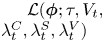 $\mathcal {L}(\boldsymbol {\phi };\tau,V_t, \lambda ^{C}_t,\lambda _t^{S},\lambda ^{V}_t)$ can be solved by the following PIDE
 \begin{align} 0& ={-}\frac{\partial \mathcal{L}}{\partial \tau} + \kappa(\theta-V_t)\frac{\partial \mathcal{L}}{\partial V_t} +\frac{1}{2}\sigma_V^{2} V_t \frac{\partial^{2} \mathcal{L}}{\partial V_t^{2}}+\alpha^{C}(\lambda^{C}_{\infty}-\lambda^{C}_t)\frac{\partial\mathcal{L}}{\partial \lambda_t^{C}}\nonumber\\ & \quad+\alpha^{S}(\lambda^{S}_{\infty}-\lambda^{S}_t)\frac{\partial \mathcal{L}}{\partial \lambda_t^{S}} +\alpha^{V}(\lambda^{V}_{\infty}-\lambda^{V}_t)\frac{\partial \mathcal{L}}{\partial \lambda_t^{V}}\nonumber\\ & \quad + \lambda_t^{C} \mathrm{E}_t^{\mathbb{Q}}(\mathcal{L}(\boldsymbol{\phi};\tau,V_t+\bar{J}^{V},\lambda_t^{C} +J_{\lambda}^{C},\lambda_t^{S},\lambda_t^{V})-\mathcal{L}(\boldsymbol{\phi};\tau,V_t,\lambda_t^{C},\lambda_t^{S},\lambda_t^{V}))\nonumber\\ & \quad + \lambda_t^{S} \mathrm{E}_t^{\mathbb{Q}}(\mathcal{L}(\boldsymbol{\phi};\tau,V_t,\lambda_t^{C},\lambda_t^{S} +J_{\lambda}^{S},\lambda_t^{V})-\mathcal{L}(\boldsymbol{\phi};\tau,V_t,\lambda_t^{C},\lambda_t^{S},\lambda_t^{V}))\nonumber\\ & \quad +\lambda_t^{V}\mathrm{E}_t^{\mathbb{Q}}(\mathcal{L}(\boldsymbol{\phi};\tau,V_t+J^{V},\lambda_t^{C},\lambda_t^{S}, \lambda_t^{V}+J_{\lambda}^{V})-\mathcal{L}(\boldsymbol{\phi};\tau,V_t,\lambda_t^{C},\lambda_t^{S},\lambda_t^{V})), \end{align}
with  $\mathcal {L}(\boldsymbol {\phi };0,V_t,\lambda ^{C}_t,\lambda _t^{S},\lambda ^{V}_t)=e^{\phi _1 V_t+\phi _2\lambda _t^{C}+\phi _3\lambda _t^{S}+\phi _4\lambda _t^{V}}$. Define
 $X_t=(\ln S_t,V_t,\lambda ^{C}_t,\lambda ^{S}_t,\lambda ^{V}_t)'$,
 $W_t=(W^{S}_t,W_t^{V},0,0,0)'$ and
 $\lambda (X_t)=(\lambda ^{C}_t,\lambda ^{S}_t,\lambda ^{V}_t)'$, and the Markov process
 $X_t$ is equivalent to
 $$\mathrm{d}X_t=(\mathcal{M}+\mathcal{K}X_t)\,\mathrm{d}t+\Sigma(X_t)\,\mathrm{d}W_t +\bar{J}\,\mathrm{d}N^{C}_t+J\,\mathrm{d}N_t,$$
where
 \begin{align*} \Sigma(X_t)& =\begin{bmatrix} \sqrt{V_t} & 0 & 0 & 0 & 0\\0 & \sigma_V\sqrt{V_t} & 0 & 0 & 0\\ 0 & 0 & 0 & 0 & 0\\ 0 & 0 & 0 & 0 & 0\\ 0 & 0 & 0 & 0 & 0 \end{bmatrix};\\ \bar{J}& =\begin{bmatrix} \bar{J^{S}} & 0 & 0 & 0 & 0\\0 & \bar{J}^{V} & 0 & 0 & 0\\0 & 0 & J_{\lambda}^{C} & 0 & 0\\0 & 0 & 0 & 0 & 0\\0 & 0 & 0 & 0 & 0\end{bmatrix};\quad J=\begin{bmatrix}J^{S} & 0 & 0 & 0 & 0\\0 & J^{V} & 0 & 0 & 0\\0 & 0 & 0 & 0 & 0\\0 & 0 & 0 & J_{\lambda}^{S} & 0\\0 & 0 & 0 & 0 & J_{\lambda}^{V}\end{bmatrix};\\ \mathrm{d}N_t^{C}& =(\mathrm{d}N_t^{C},\mathrm{d}N_t^{C},\mathrm{d}N_t^{C},0,0)';\quad \mathrm{d}N_t=(\mathrm{d}N_t^{S},\mathrm{d}N_t^{V},0,\mathrm{d}N_t^{S},\mathrm{d}N_t^{V})'. \end{align*}
The affine dependence of  $\mathcal {M}$,
 $\mathcal {K}$,
 $\Sigma (X_t)\Sigma (X_t)'$ and
 $\lambda (X_t)$ is given by
 \begin{align*} \mathcal{M}& =(r-q,\kappa\theta,\alpha^{C}\lambda_{\infty}^{C},\alpha^{S}\lambda_{\infty}^{S},\alpha^{V}\lambda_{\infty}^{V})',\\ \mathcal{K}& =\begin{bmatrix} 0 & -\frac 12 & -\bar{\zeta} & -\zeta & 0\\ 0 & -\kappa & 0 & 0 & 0\\ 0 & 0 & -\alpha^{C} & 0 & 0\\ 0 & 0 & 0 & -\alpha^{S} & 0\\ 0 & 0 & 0 & 0 & -\alpha^{V} \end{bmatrix},\\ \Sigma(X_t)\Sigma(X_t)'& =\begin{bmatrix} V_t & 0 & 0 & 0 & 0\\ 0 & \sigma_V^{2}V_t & 0 & 0 & 0\\ 0 & 0 & 0 & 0 & 0\\ 0 & 0 & 0 & 0 & 0\\ 0 & 0 & 0 & 0 & 0 \end{bmatrix}=H V_t,\quad \text{where } H=\begin{bmatrix} 1 & 0 & 0 & 0 & 0\\ 0 & \sigma_V^{2} & 0 & 0 & 0\\ 0 & 0 & 0 & 0 & 0\\ 0 & 0 & 0 & 0 & 0\\0 & 0 & 0 & 0 & 0\end{bmatrix}. \end{align*}
Thanks to the affine structure in the SVCIJ-H model, the solution to this PIDE can be written in the following form
 \begin{equation} \mathcal{L}(\boldsymbol{\phi};\tau,V_t,\lambda^{C}_t,\lambda_t^{S},\lambda^{V}_t) = e^{h_1(\boldsymbol{\phi};\tau)V_t + h_2(\boldsymbol{\phi};\tau)\lambda^{C}_t+h_3(\boldsymbol{\phi};\tau)\lambda^{S}_t+h_4(\boldsymbol{\phi};\tau)\lambda_t^{V} +h_5(\boldsymbol{\phi};\tau)}. \end{equation}
Substituting Eq. (B.7) into PDE (B.6), we have
 \begin{align} 0& ={-}\left(V_t\frac{\partial}{\partial\tau}h_1(\boldsymbol{\phi},\tau) +\lambda^{C}_t\frac{\partial}{\partial\tau}h_2(\boldsymbol{\phi},\tau) +\lambda^{S}_t\frac{\partial}{\partial\tau}h_3(\boldsymbol{\phi},\tau) +\lambda^{V}_t\frac{\partial}{\partial\tau}h_4(\boldsymbol{\phi},\tau) +\frac{\partial}{\partial\tau}h_5(\boldsymbol{\phi},\tau)\right)\nonumber\\ & \quad + \kappa(\theta-V_t)h_1(\boldsymbol{\phi},\tau)+\frac{1}{2}\sigma_V^{2} V_t h_1^{2}(\boldsymbol{\phi},\tau)+\alpha^{C}(\lambda^{C}_{\infty}-\lambda^{C}_t)h_2(\boldsymbol{\phi},\tau) +\alpha^{S}(\lambda^{S}_{\infty}-\lambda^{S}_t)h_3(\boldsymbol{\phi},\tau)\nonumber\\ & \quad +\alpha^{V}(\lambda^{V}_{\infty}-\lambda^{V}_t)h_4(\boldsymbol{\phi},\tau)+ \lambda_t^{C} \mathrm{E}_t^{\mathbb{Q}}(e^{\bar{J}^{V}h_1(\boldsymbol{\phi},\tau)+J_{\lambda}^{C}h_2(\boldsymbol{\phi},\tau)}-1) + \lambda_t^{S} \mathrm{E}_t^{\mathbb{Q}}(e^{J_{\lambda}^{S}h_3(\boldsymbol{\phi},\tau)}-1)\nonumber\\ & \quad +\lambda_t^{V} \mathrm{E}_t^{\mathbb{Q}}(e^{J^{V}h_1(\boldsymbol{\phi},\tau)+J_{\lambda}^{V}h_4(\boldsymbol{\phi},\tau)}-1). \end{align}
Since PDE (B.8) holds for all arbitrary  $t$,
 $V_t$,
 $\lambda ^{C}_t$,
 $\lambda ^{S}_t$ and
 $\lambda ^{V}_t$, this reduces the problem to solving four much simpler ODEs:
 $$\left\{ \begin{aligned} \frac{\partial}{\partial\tau}h_1(\boldsymbol{\phi},\tau) & ={-}\kappa h_1(\boldsymbol{\phi},\tau)+\frac{1}{2}\sigma_V^{2} h_1^{2}(\boldsymbol{\phi},t),\\ \frac{\partial}{\partial\tau}h_2(\boldsymbol{\phi},\tau) & ={-}\alpha^{C} h_2(\boldsymbol{\phi},\tau) +\frac{1}{1-\bar{\mu}_Vh_1(\boldsymbol{\phi},\tau)}\times\frac{1}{1-\mu_{\lambda}^{C}h_2(\boldsymbol{\phi},\tau)}-1,\\ \frac{\partial}{\partial\tau}h_3(\boldsymbol{\phi},\tau) & ={-}\alpha^{S} h_3(\boldsymbol{\phi},\tau) +\frac{1}{1-\mu_{\lambda}^{S}h_3(\boldsymbol{\phi},\tau)}-1,\\ \frac{\partial}{\partial\tau}h_4(\boldsymbol{\phi},\tau) & ={-}\alpha^{V} h_4(\boldsymbol{\phi},\tau) +\frac{1}{1-\mu_Vh_1(\boldsymbol{\phi},\tau)}\times\frac{1}{1-\mu_{\lambda}^{V}h_4(\boldsymbol{\phi},\tau)}-1,\\ \frac{\partial}{\partial\tau}h_5(\boldsymbol{\phi},\tau) & = \kappa\theta h_1(\boldsymbol{\phi},\tau)+\alpha^{C}\lambda^{C}_{\infty} h_2(\boldsymbol{\phi},\tau) + \alpha^{S}\lambda^{S}_{\infty} h_3(\boldsymbol{\phi},\tau)+ \alpha^{V}\lambda^{V}_{\infty} h_4(\boldsymbol{\phi},\tau), \end{aligned} \right.$$
with the initial conditions
 $$h_1(\boldsymbol{\phi},0)=\phi_1,\quad h_2(\boldsymbol{\phi},0)=\phi_2,\quad h_3(\boldsymbol{\phi},0)=\phi_3,\quad h_4(\boldsymbol{\phi},0)=\phi_4,\quad h_5(\boldsymbol{\phi},0)=0.$$
The solutions to the Riccati equation of  $h_1(\boldsymbol {\phi },\tau )$ is
 $$h_1(\boldsymbol{\phi},\tau)= \frac{2\kappa \phi_1}{\sigma_V^{2}\phi_1+(2\kappa-\sigma_V^{2}\phi_1)e^{\kappa \tau}}.$$
The ODEs cannot be solved in closed form except for  $h_1(\boldsymbol {\phi },\tau )$, but they can be solved numerically.
Proof of Lemma 1. Proof of Lemma 1.
For the SVCIJ-H model, given  $0< t< s$, by applying Itô's Lemma to
 $e^{\kappa t}\lambda _t^{i}$ (
 $i\in \{C,~S,~V\}$) we obtain
 $$\lambda^{i}_s=\lambda_t^{i} e^{-\alpha^{i}(s-t)}+\lambda_{\infty}^{i}(1-e^{-\alpha^{i}(s-t)}) +\int_t^{s}e^{-\alpha^{i}(s-u)}J_{\lambda}^{i}\,\mathrm{d}N_u^{i},$$
and the conditional expectation of  $\lambda ^{i}_s$ on
 $\mathcal {F}$ under the risk-neutral measure is
 \begin{equation} \mathbb{E}_t(\lambda_s^{i})=\lambda_t^{i}e^{-(\alpha^{i}-\mu_{\lambda}^{i})(s-t)} +\tilde{\lambda}^{i}[1-e^{-(\alpha^{i}-\mu_{\lambda}^{i})(s-t)}],\end{equation}
where 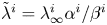 $\tilde {\lambda }^{i}=\lambda _{\infty }^{i}\alpha ^{i}/\beta ^{i}$ and
 $\beta ^{i}=\alpha ^{i}-\mu _{\lambda }^{i}>0$. Then, Eq. (B.9), an application of Itô's Lemma under the risk-neutral measure to obtain
 $\mathrm {d}(e^{\kappa t}V_t)$ and then integrating, and an application of the law of iterated expectations together imply
 \begin{align*} \mathbb{E}_t(V_s)& =V_te^{-\kappa(s-t)}+\theta(1-e^{-\kappa(s-t)})\\ & \quad +\bar{\mu}_V\left[\frac{\lambda_t^{C}-\tilde{\lambda}^{C}}{\kappa-\beta^{C}}(e^{-\beta^{C}(s-t)}-e^{-\kappa(s-t)}) +\frac{\tilde{\lambda}^{C}}{\kappa}(1-e^{-\kappa(s-t)})\right]\\ & \quad +\mu_V\left[\frac{\lambda_t^{V}-\tilde{\lambda}^{V}}{\kappa-\beta^{V}}(e^{-\beta^{V}(s-t)}-e^{-\kappa(s-t)}) +\frac{\tilde{\lambda}^{V}}{\kappa}(1-e^{-\kappa(s-t)})\right]. \end{align*}
Notably,  $\mathbb {E}_t(\lambda _s^{i})$ and
 $\mathbb {E}_t(V_s)$ are both increasing in
 $s$. Finally, for
 $\kappa \neq \alpha$,
 \begin{align*} \frac{1}{\tilde{\tau}}\mathbb{E}_t\left(\int_t^{t+\tilde{\tau}}V_s \,\mathrm{d}s\right)& =\varphi(\tilde{\tau})V_t+\theta(1-\varphi(\tilde{\tau})) +\bar{\mu}_V\left[\frac{\lambda_t^{C}-\tilde{\lambda}^{C}}{\kappa-\beta^{C}}(\varphi(\beta^{C}) -\varphi(\tilde{\tau}))+\frac{\tilde{\lambda}^{C}}{\kappa}(1-\varphi(\tilde{\tau}))\right]\\ & \quad +\mu_V\left[\frac{\lambda_t^{V}-\tilde{\lambda}^{V}}{\kappa-\beta^{V}}(\varphi(\beta^{V}) -\varphi(\tilde{\tau}))+\frac{\tilde{\lambda}^{V}}{\kappa}(1-\varphi(\tilde{\tau}))\right], \end{align*}
where  $\varphi (x)={(1-e^{-x\tilde {\tau }})}/{x\tilde {\tau }}$. The definition of the CBOE VIX formula is
 \begin{align} \text{VIX}_t^{2}(\tilde{\tau})& =\frac{2}{\tilde{\tau}}\mathbb{E}_t \left[\int_t^{t+\tilde{\tau}}\left(\frac{\mathrm{d}S_u}{S_u}-\mathrm{d}\log S_u\right)\right]\nonumber\\ & =\frac{1}{\tilde{\tau}}\mathbb{E}_t\left(\int_t^{t+\tilde{\tau}}V_u\, \mathrm{d}u\right)+\frac{2}{\tilde{\tau}}\mathbb{E}\left(\int_t^{t+\tilde{\tau}} (e^{\bar{J}_S}-\bar{J}_S-1)\,\mathrm{d}N_u^{C}\right)\nonumber\\ & \quad+\frac{2}{\tilde{\tau}}\mathbb{E} \left(\int_t^{t+\tilde{\tau}}(e^{J_S}-J_S-1)\,\mathrm{d}N_u^{S}\right)\nonumber\\ & =V_t\varphi(\tilde{\tau})+\lambda^{C}_t\left[\frac{\bar{\mu}_V(\varphi(\beta^{C})-a)}{\kappa-\beta^{C}}+2\varphi(\beta^{C}) (\bar{\zeta}- \bar{\mu}_S-\rho_J\bar{\mu}_V)\right]+\lambda^{S}_t[2\varphi(\beta^{S})(\zeta - \mu_S)]\nonumber\\ & \quad +\lambda^{V}_t\left[\frac{\mu_V(\varphi(\beta^{V})-a)}{\kappa-\beta^{V}}\right] +\left(\theta+\frac{\tilde{\lambda}^{C}\bar{\mu}_V + \tilde{\lambda}^{V} \mu_V}{\kappa}\right)(1-a)\nonumber\\ & \quad +2 \tilde{\lambda}^{C} (\bar{\zeta} - \bar{\mu}_S-\rho_J \bar{\mu}_V)(1-\varphi(\beta^{C}))+2\tilde{\lambda}^{S} (\zeta - \mu_S )(1-\varphi(\beta^{S}))\nonumber\\ & \quad - \frac{\bar{\mu}_V\tilde{\lambda}^{C}}{\kappa-\beta^{C}}(\varphi(\beta^{C})-a)- \frac{\mu_V\tilde{\lambda}^{V}}{\kappa-\beta^{V}}(\varphi(\beta^{V})-a). \end{align}
For the SVCIJ-I model, we obtain
 $$\mathbb{E}_t(V_s) =V_te^{{-}A\tilde{\tau}}+\frac{B}{A}-\frac{B}{A}e^{{-}A\tilde{\tau}},$$
where  $A=\kappa -\lambda ^{2,V}\mu _V-\lambda ^{2,C}\bar {\mu }_V$ and
 $B=\theta \kappa +\lambda ^{1,V}\mu _V+\lambda ^{1,C}\bar {\mu }_V$, and then
 \begin{align*} \text{VIX}_t^{2}(\tilde{\tau})& =\frac{1}{\tilde{\tau}}\mathbb{E}_t\left(\int_t^{t+\tilde{\tau}}V_u \mathrm{d}u\right)+\frac{2}{\tilde{\tau}}\mathbb{E}\left(\int_t^{t+\tilde{\tau}} (e^{\bar{J}_S}-\bar{J}_S-1)\,\mathrm{d}N_u^{C}\right)\\ & \quad +\frac{2}{\tilde{\tau}}\mathbb{E} \left(\int_t^{t+\tilde{\tau}}(e^{J_S}-J_S-1)\,\mathrm{d}N_u^{S}\right)\\ & =V_t\eta[1+2\lambda^{2,C}(\bar{\zeta} - \bar{\mu}_S-\rho_J \bar{\mu}_V)+2\lambda^{2,S}(\zeta - \mu_S)]+\frac{B}{A}(1-\eta) \\ & \quad +2(\bar{\zeta} - \bar{\mu}_S-\rho_J \bar{\mu}_V)\left[\lambda^{1,C}+\lambda^{2,C}\frac{B}{A}(1-\eta)\right] + 2(\zeta - \mu_S )\left[\lambda^{1,S}+\lambda^{2,S}\frac{B}{A}(1-\eta)\right]. \end{align*}
Proof of Theorem 1. Proof of Theorem 1.
Using the transform (4), the pricing problem of VIX futures can be computed as follows:
 \begin{equation} F(T)=\mathbb{E}[\text{VIX}_T]=\frac{1}{2\sqrt{\pi}}\int_0^{\infty} \frac{1-\mathbb{E}(e^{{-}s\text{VIX}_T^{2}})}{s^{3/2}}\,\mathrm{d} s, \end{equation}
where  $s\in \mathbb {R^{+}}$. Fortunately, we know the relationship between VIX square and state variables (see Lemma 1), so the above formula can be calculated. Specifically, for SVCIJ-I model, the pricing formula can be transformed into
 \begin{equation} F(T)=\frac{1}{2\sqrt{\pi}}\int_0^{\infty} \frac{1-\mathbb{E}(e^{{-}s(aV_T+b)})}{s^{3/2}}\,\mathrm{d} s. \end{equation}
For the SVCIJ-H model, the pricing formula can be transformed into
 \begin{equation} F(T)=\frac{1}{2\sqrt{\pi}}\int_0^{\infty} \frac{1-\mathbb{E}(e^{{-}s(aV_T+b\lambda_T^{C}+c\lambda_T^{S}+d\lambda_T^{V}+e)})}{s^{3/2}}\,\mathrm{d} s. \end{equation}
Proof of Theorem 2. Proof of Theorem 2.
Using the transform (5), the pricing problem of VIX options can be computed as follows:
 \begin{equation} C(T,K) =\mathbb{E}[(\text{VIX}_T-K)^{+}]=\frac{e^{{-}rT}}{2\sqrt{\pi}}\int_0^{\infty} \operatorname{Re}\left[\frac{1-\text{erf}(K\sqrt{\phi})}{\phi^{3/2}}\mathbb{E}(e^{\phi \text{VIX}_T^{2}})\right]\mathrm{d}\phi_I, \end{equation}
where  $\phi =\phi _R+i\phi _I\in Z$,
 $\phi _I\in \mathbb {R}$ and
 $\phi _I\in \mathbb {R}^{+}$. Fortunately, we know the relationship between VIX square and state variables (see Lemma 1), so the above formula can be calculated. Specifically, for SVCIJ-I model, the pricing formula can be transformed into
 \begin{equation} C(T,K) =\frac{e^{{-}rT}}{2\sqrt{\pi}}\int_0^{\infty} \operatorname{Re}\left[\frac{1-\text{erf}(K\sqrt{\phi})}{\phi^{3/2}}\mathbb{E}(e^{\phi (aV_T+b)})\right]\mathrm{d}\phi_I. \end{equation}
For the SVCIJ-H model, the pricing formula can be transformed into
 \begin{equation} C(T,K) =\frac{e^{{-}rT}}{2\sqrt{\pi}}\int_0^{\infty} \operatorname{Re}\left[\frac{1-\text{erf}(K\sqrt{\phi})}{\phi^{3/2}}\mathbb{E}(e^{\phi (aV_T+b\lambda_T^{C}+c\lambda_T^{S}+d\lambda_T^{V}+e)})\right]\mathrm{d}\phi_I. \end{equation}