1 Introduction
The Fourier law of heat conduction is one of the foundations of transport theory in the realm of continuum mechanics. The law states that the heat flux in the continuum regime is proportional to the magnitude of the temperature gradient, but opposite in direction, often called counter-gradient transport. It is known that deviations from the Fourier law occur outside the continuum regime. Flows in microscale devices often fall into the rarefied realm as the device size is not substantially larger than the mean free path of the gas. In many high-altitude flight applications, the flow is not only rarefied, but also compressible and in a state of thermodynamic non-equilibrium. Throughout this work the term thermodynamic non-equilibrium indicates a gas flow whose constituent molecular velocity distribution function is far from a Maxwellian. Thus, there is much fundamental interest in understanding and characterizing thermal transport in rarefied gas flows in various speed regimes far from thermodynamic equilibrium.
Lid-driven cavity flow is ideally suited for examining non-equilibrium rarefied effects as it incorporates important physics within a simple geometry. Microcavity flows are encountered in many MEMS (micro electro-mechanical systems) applications. In these systems, the overall device performance depends critically on the transport (mixing) within the cavity. Microcavity flows are also of interest in the study of thermal protection system of space re-entry vehicles. Slits, suction chambers, impact damage or any other pockets on the surface of a re-entry flight vehicle can be conveniently modelled as cavities of different sizes and shapes. In high-speed re-entry flows, the free stream may be rarefied but the flow within the cavity could be close to continuum due to the accumulation of trapped molecules. According to Bertin & Cummings (Reference Bertin and Cummings2006), one of the main reasons for the failure of the NASA space shuttle Columbia was the breaching of hot gas through cavities in the thermal protection system of the vehicle during its re-entry. Evidently, it is important to characterize the thermal transport in cavities of different shapes and sizes as a function of flow speed and degree of rarefaction.
The Knudsen number is the dimensionless parameter that characterizes the degree of rarefaction of a given flow field. The Knudsen number based on the density gradient (
 $\unicode[STIX]{x1D735}\unicode[STIX]{x1D70C}$
) is widely used to examine non-equilibrium effects due to rarefaction:
 $$\begin{eqnarray}\displaystyle Kn_{local}=\frac{\unicode[STIX]{x1D706}}{l_{\unicode[STIX]{x1D70C}}},\quad \text{where }l_{\unicode[STIX]{x1D70C}}=\frac{\unicode[STIX]{x1D70C}}{|\unicode[STIX]{x1D735}\unicode[STIX]{x1D70C}|}, & & \displaystyle\end{eqnarray}$$
and
 $\unicode[STIX]{x1D706}$
is the mean free path.
The well-known Navier–Stokes–Fourier (NS–F) equations are generally inapplicable beyond a local Knudsen number of approximately
 $0.01$
. Extended hydrodynamic equations such as the Burnett or super-Burnett equations further the applicability of the constitutive relations to a broader range of Knudsen numbers. The high degrees of rarefaction encountered in MEMS devices and high-altitude flight may fall outside the range of applicability of extended thermodynamic models. In highly rarefied regimes, the flow field is governed by the kinetic Boltzmann equation which describes the evolution of the single particle velocity distribution function (v.d.f.). Rather than using the constitutive relations, the transport fluxes are calculated directly from the moments of the v.d.f. leading to a much wider range of applicability.
The objective of the study is to characterize thermal transport as a function of the Knudsen and Mach numbers. We examine the thermal transport behaviour within a canonical lid-driven cavity flow experiencing a high degree of non-equilibrium (rarefaction) using kinetic approaches. Solving the complete Boltzmann equation is neither feasible nor necessary for the flow regimes of interest. Instead, we use two simplified kinetic models that retain much of the relevant physics. Direct simulation Monte Carlo (DSMC) is an excellent numerical approximation of the Boltzmann equation for the purpose of this study. It is computationally viable for a high degree of rarefaction (free molecular regime), but too expensive for moderate levels. The principal kinetic approach employed in the study is called the unified gas kinetic scheme (UGKS). This scheme is computationally more viable than DSMC over a wide range of Knudsen numbers. The approximations to the Boltzmann equation leading to DSMC and UGKS will be discussed in later sections. Thermal flux is computed in UGKS by integrating over the velocity distribution function. Before examining the heat transport, UGKS results are verified against DSMC computations over a range of transition-to-rarefied Knudsen numbers to ensure that the flow physics of interest is adequately captured. UGKS has already been verified in near-equilibrium flows in previous studies (Venugopal & Girimaji Reference Venugopal and Girimaji2015).
This work focuses on two foundational aspects of thermal transport in a rarefied medium: (i) the alignment of the UGKS thermal flux relative to the temperature gradient and predictions of two extended thermodynamic models; and (ii) entropy analyses at different Mach and Knudsen numbers. The UGKS fluxes are compared against closed analytical constitutive relations from the Fourier law and extended thermodynamic models – the Burnett (Yun et al.
Reference Yun, Agarwal, Balakrishnan, Yun, Agarwal and Balakrishnan1997) and Bhatnagar–Gross–Krook–Burnett (BGK-Burnett) models (Agarwal & Balakrishnan Reference Agarwal and Balakrishnan1996). Regimes of validity of these models are discussed. The entropy characteristics are examined at different degrees of rarefaction against two different entropy formulations: (i) the Sackur–Tetrode equation and (ii) the Boltzmann
 $H$
-theorem.
The remainder of the paper is arranged as follows. The kinetic Boltzmann equation is presented in § 2. A brief description of DSMC and a detailed account of UGKS are also provided in § 2. Section 3 contains the description of thermodynamic models used in the current study. Section 3 also presents continuum and kinetic entropy formulations. The details of the rarefied cavity numerical simulations are given in § 4. Verification studies of UGKS implementation performed by comparing against the DSMC are also presented in § 4. The thermal flux results are given in § 5 along with a discussion of the various ramifications of the findings. We conclude in § 6 with a summary.
2 Kinetic equations and computational models
Here, we present the kinetic equations, approximations and numerical approaches used in this study. The kinetic Boltzmann equation describes the evolution of the particle velocity distribution function
 $f$
in phase space (
 $x_{1},x_{2},x_{3},u_{1},u_{2},u_{3},t$
):
 $$\begin{eqnarray}\displaystyle \frac{\unicode[STIX]{x2202}(f)}{\unicode[STIX]{x2202}t}+u_{j}\frac{\unicode[STIX]{x2202}(f)}{\unicode[STIX]{x2202}x_{j}}+\frac{\unicode[STIX]{x2202}(F_{j}\,f)}{\unicode[STIX]{x2202}u_{j}}=Q, & & \displaystyle\end{eqnarray}$$
where,
 $\boldsymbol{x}$
is the position vector,
 $\boldsymbol{u}$
is the particle velocity and
 $\boldsymbol{F}$
is any external force per unit mass such as the acceleration due to gravity.
 $Q$
is the nonlinear collision operator. The mathematical form of
 $Q$
depends on the type of collisions and the Knudsen number. Under molecular chaos assumptions,
 $Q$
can be written as an integral of the product of pre- and post-collision distribution functions over velocity space. This makes the Boltzmann equation an integro-differential equation and therefore not amenable to simple analyses and computations. Simplifications to the collision operator can be invoked depending upon the degree of rarefaction, to allow for efficient numerical simulations.
2.1 Near-equilibrium regime
In the near-continuum regime, the complex collision operator can be simplified using a model proposed by Bhatnagar, Gross & Krook (Reference Bhatnagar, Gross and Krook1954). This collision operator, often known as the BGK collision model, is given by:
 $$\begin{eqnarray}\displaystyle Q=\frac{g-f}{\unicode[STIX]{x1D70F}}. & & \displaystyle\end{eqnarray}$$
The resulting kinetic equation is known as the Boltzmann-BGK (B-BGK) equation:
 $$\begin{eqnarray}\displaystyle \frac{\unicode[STIX]{x2202}(f)}{\unicode[STIX]{x2202}t}+u_{j}\frac{\unicode[STIX]{x2202}(f)}{\unicode[STIX]{x2202}x_{j}}+\frac{\unicode[STIX]{x2202}(F_{j}f)}{\unicode[STIX]{x2202}u_{j}}=\frac{g-f}{\unicode[STIX]{x1D70F}}. & & \displaystyle\end{eqnarray}$$
Here,
 $g$
is the Maxwellian distribution function that is unique for a given density (
 $\unicode[STIX]{x1D70C}$
), mean velocity (
 $\boldsymbol{U}$
) and temperature (
 $T$
); and
 $\unicode[STIX]{x1D70F}$
is the mean collision time that is inversely proportional to density (
 $\unicode[STIX]{x1D70C}$
) and can have a dependence on temperature. The B-BGK equation can be thought of as a mathematical model that describes the relaxation of a mildly non-equilibrium distribution (
 $f$
) towards the equilibrium distribution (
 $g$
) with a local relaxation time of
 $\unicode[STIX]{x1D70F}$
.
The B-BGK equation permits a solution through the method of characteristics which enables numerical simulation of a variety of flows of interest (Prendergast & Xu Reference Prendergast and Xu1993). This solution is utilized in constructing fluxes for finite volume schemes. Such an approach is called the gas kinetic scheme (GKS) and has been well developed by several authors – see for example Xu (Reference Xu2001), Xu & He (Reference Xu and He2003), Xu, Mao & Tang (Reference Xu, Mao and Tang2005), Kerimo & Girimaji (Reference Kerimo and Girimaji2007), May, Srinivasan & Jameson (Reference May, Srinivasan and Jameson2007), Kumar, Girimaji & Kerimo (Reference Kumar, Girimaji and Kerimo2013). A brief description of the GKS is given below.
For simplicity, we start from the one-dimensional B-BGK equation:
 $$\begin{eqnarray}\displaystyle \unicode[STIX]{x2202}_{t}f+u\unicode[STIX]{x2202}_{x}f=\frac{g-f}{\unicode[STIX]{x1D70F}}, & & \displaystyle\end{eqnarray}$$
where, the Maxwellian distribution,
 $g$
, is given by:
 $$\begin{eqnarray}\displaystyle g=\unicode[STIX]{x1D70C}\left(\frac{m}{2\unicode[STIX]{x03C0}k_{B}T}\right)^{(K+1)/2}\exp \left(-\frac{m}{2k_{B}T}((u-U)^{2}+\unicode[STIX]{x1D701}^{2})\right), & & \displaystyle\end{eqnarray}$$
where,
 $m$
is the molecular mass,
 $k_{B}$
is the Boltzmann constant,
 $U$
is the macroscopic fluid velocity,
 $K$
is the number of internal degrees of freedom and
 $\unicode[STIX]{x1D701}^{2}=\sum _{i=1}^{K}\unicode[STIX]{x1D701}_{i}^{2}$
is the energy associated with the internal degrees of freedom,
 $u$
is the particle velocity and
 $T$
is the temperature. The exponent
 $K+1$
indicates that we chose a one-dimensional (1-D) gas flow with one velocity component. For 3-D flows, the exponent would be
 $K+3$
;
 $\unicode[STIX]{x1D70C}$
,
 $U$
and
 $T$
are the moments of
 $g$
.
Consider solving equation (2.4) for the 1-D case on a finite volume grid where we compute the conserved variables at the cell centres (
 $x_{i}$
) and fluxes at the interfaces between the cells (
 $x_{i-1/2}$
), where,
 $$\begin{eqnarray}\displaystyle x_{i}=(i-1/2)\unicode[STIX]{x0394}x;\quad x_{i-1/2}=(i-1)\unicode[STIX]{x0394}x. & & \displaystyle\end{eqnarray}$$
The solution to the equilibrium distribution function at the cell interface is obtained via the method of characteristics:
 $$\begin{eqnarray}\displaystyle f(x_{j+1/2},t^{n+1},u,\unicode[STIX]{x1D701}) & = & \displaystyle \frac{1}{\unicode[STIX]{x1D70F}}\int _{t^{n}}^{t^{n+1}}g(x_{j+1/2}-u(t-t^{\prime }),t^{\prime },u,\unicode[STIX]{x1D701})\text{e}^{(t^{\prime }-t)/\unicode[STIX]{x1D70F}}\,\text{d}t^{\prime }\nonumber\\ \displaystyle & & \displaystyle +\,\text{e}^{(t^{n}-t)/\unicode[STIX]{x1D70F}}f_{0}^{n}(x_{j+1/2}-u(t-t^{n}),t^{n},u,\unicode[STIX]{x1D701}),\end{eqnarray}$$
where
 $f_{0}^{n}$
is the initial distribution function at
 $t^{n}$
and
 $n$
indicates the time step level. Nonlinear interpolation is applied to obtain
 $f_{0}^{n}$
, which is considered to be piecewise continuous in each cell and to have different slopes to the left and right of the interface at
 $x_{j+1/2}$
. The equilibrium distribution function,
 $g$
, can be obtained from
 $f_{0}^{n}$
by invoking the compatibility condition:
 $$\begin{eqnarray}\displaystyle \lim _{t\rightarrow 0}\int (g-f)\unicode[STIX]{x1D74D}\,\text{d}\unicode[STIX]{x1D6EF}=0, & & \displaystyle\end{eqnarray}$$
where,
 $\unicode[STIX]{x1D74D}=(1,u,0.5(u^{2}+\unicode[STIX]{x1D701}^{2}))^{T}$
are the collision invariants and
 $\text{d}\unicode[STIX]{x1D6EF}=\text{d}u\,\text{d}\unicode[STIX]{x1D701}_{1}\,\text{d}\unicode[STIX]{x1D701}_{2}\ldots \text{d}\unicode[STIX]{x1D701}_{k}$
. This implies that the moments of the collision term about the collision invariants must vanish in order to satisfy the conservation laws. Once
 $f_{0}^{n}$
and
 $g$
are determined, the fluxes are determined by taking the moments of equation (2.7) without having to explicitly determine the distribution function at the interface (Xu Reference Xu2001).
For a full three-dimensional formulation, the vector of conserved variables and fluxes can be determined from the distribution function as follows:
 $$\begin{eqnarray}\displaystyle \boldsymbol{W}=(\unicode[STIX]{x1D70C},\unicode[STIX]{x1D70C}\boldsymbol{U},\unicode[STIX]{x1D70C}e)^{T}=\int f\unicode[STIX]{x1D74D}\,\text{d}\unicode[STIX]{x1D6EF};\quad \boldsymbol{F}=\int _{t^{n}}^{t^{n+1}}\int \unicode[STIX]{x1D74D}f\boldsymbol{u}\,\text{d}\unicode[STIX]{x1D6EF}\,\text{d}t. & & \displaystyle\end{eqnarray}$$
Now, the conserved variables at the new time step can be computed using:
 $$\begin{eqnarray}\displaystyle \boldsymbol{W}_{i}^{n+1}=\boldsymbol{W}_{i}^{n}+\frac{1}{\unicode[STIX]{x0394}x}(\boldsymbol{F}_{i-1/2}-\boldsymbol{F}_{i+1/2}). & & \displaystyle\end{eqnarray}$$
The fluxes defined above contain both convective transport due to the macroscopic velocity (
 $\boldsymbol{U}$
) as well as molecular transport due to the peculiar velocity (
 $\boldsymbol{u}-\boldsymbol{U}$
). The molecular heat flux (thermal transport) is obtained by subtracting the convective contribution from the total flux:
 $$\begin{eqnarray}\displaystyle \boldsymbol{q}=\int \frac{1}{2}mf(\boldsymbol{u}-\boldsymbol{U})[(\boldsymbol{u}-\boldsymbol{U})\boldsymbol{\cdot }(\boldsymbol{u}-\boldsymbol{U})]\,\text{d}\unicode[STIX]{x1D6EF}. & & \displaystyle\end{eqnarray}$$
The advantage of the GKS is that the macroscopic variables can be obtained directly using closed form expressions for the moments of the Maxwell distribution function. The underlying distribution function is not calculated explicitly. In general, the GKS is not applicable for the transition or rarefied regime as it cannot accommodate large departures of the v.d.f. from a Maxwellian. Thus, the GKS is not adequate for the present study.
2.2 Transition and rarefied regime
We now present simplifications to the kinetic Boltzmann equation suitable in the transition/rarefied regime. Two such approximate methods are employed in this study – the unified gas kinetic scheme (UGKS) and direct simulation Monte Carlo (DSMC). UGKS falls into the category of discrete velocity methods (DVM) or discrete ordinate methods (DOM). DSMC is a stochastic approximation to the kinetic equation. Detailed discussions of above two methods can be found in Bird (Reference Bird1994) and Xu & Huang (Reference Xu and Huang2010). Here, we present a brief description of the two methods.
2.2.1 Unified gas kinetic scheme
UGKS (Xu & Huang Reference Xu and Huang2010; Huang, Xu & Yu Reference Huang, Xu and Yu2012, Reference Huang, Xu and Yu2013) is a version of the discrete ordinate method which utilizes GKS techniques to compute fluxes of individual ordinates. For the sake of simplicity, we describe the one-dimensional version of UGKS in the following.
The velocity space in the DOM approach is discretized into
 $2M+1$
cells each of size
 $\unicode[STIX]{x0394}u$
. In the
 $k$
th velocity cell, the particle velocity assumes a value in the range:
 $$\begin{eqnarray}\displaystyle u_{k}\in [(k-1/2)\unicode[STIX]{x0394}u,(k+1/2)\unicode[STIX]{x0394}u]. & & \displaystyle\end{eqnarray}$$
A separate velocity distribution function is considered for each velocity ordinate. The gas distribution function in the finite volume cell around
 $x_{j}$
with discrete velocity
 $u_{k}$
at time
 $t^{n}$
is defined as:
 $$\begin{eqnarray}\displaystyle f(x_{j},t^{n},u_{k})\equiv f_{j,k}^{n}\equiv \frac{1}{\unicode[STIX]{x0394}x\unicode[STIX]{x0394}u}\int _{x_{j-1/2}}^{x_{j+1/2}}\int _{u_{k}-\unicode[STIX]{x0394}u/2}^{u_{k}+\unicode[STIX]{x0394}u/2}f(x,t^{n},u)\,\text{d}x\,\text{d}u, & & \displaystyle\end{eqnarray}$$
where,
 $f(x_{j},t^{n},u_{k})$
is the full particle v.d.f. Thus the overall v.d.f. can be decomposed into a series of v.d.f.s, each representing the distribution function about the ordinate value.
In the rarefied regime, the total v.d.f. is far from Gaussian and the collision operator is not amenable to the BGK approximation. However, the evolution of individual ordinate v.d.f.s can be reasonably described by the B-BGK equation as the distribution only spans a narrow range of velocities. Thus, upon discretization of the velocity space, a methodology similar to GKS can be adopted for each discretized velocity. Such an approach allows for an accurate description of discontinuous velocity distribution functions in the rarefied regime. Once the individual ordinate v.d.f.s are known, the total v.d.f. can be computed.
For UGKS, we employ the BGK-Shakhov model (Shakhov Reference Shakhov1968) to account for Prandtl number effects rather than the original B-BGK collision operator for individual ordinate v.d.f.s:
 $$\begin{eqnarray}\displaystyle Q=\frac{f^{+}-f}{\unicode[STIX]{x1D70F}}. & & \displaystyle\end{eqnarray}$$
Here
 $f^{+}$
is a modified equilibrium distribution function that can accommodate a non-unity Prandtl number. It must be noted that the original B-BGK model restricts the Prandtl number to unity.
 $$\begin{eqnarray}\displaystyle f^{+}=g\left[1+(1-Pr)\boldsymbol{c}\boldsymbol{\cdot }\boldsymbol{q}\left.\left(\frac{c^{2}}{RT}-5\right)\right/(5pRT)\right], & & \displaystyle\end{eqnarray}$$
where,
 $Pr,\boldsymbol{c}$
and
 $\boldsymbol{q}$
are the Prandtl number, peculiar velocity and heat flux, respectively.
The kinetic equation for
 $f_{j,k}^{n}$
can be written as follows (Xu & Huang Reference Xu and Huang2010):
 $$\begin{eqnarray}\displaystyle f_{j,k}^{n+1}=f_{j,k}^{n}+\frac{1}{\unicode[STIX]{x0394}x}\int (u_{k}\hat{f}_{j-1/2,k}-u_{k}\hat{f}_{j+1/2,k})\,\text{d}t+\frac{1}{\unicode[STIX]{x0394}x}\int \int \frac{f^{+}-f}{\unicode[STIX]{x1D70F}}\,\text{d}x\,\text{d}t. & & \displaystyle\end{eqnarray}$$
The distribution function at the cell interface,
 $\hat{f}_{j+1/2,k}$
, can be determined using the method of characteristics:
 $$\begin{eqnarray}\displaystyle \hat{f}_{j+1/2,k} & = & \displaystyle \hat{f}(x_{j+1/2},t,u_{k},\unicode[STIX]{x1D709})=\frac{1}{\unicode[STIX]{x1D70F}}\int _{t^{n}}^{t}f^{+}(x^{\prime },t^{\prime },u_{k},\unicode[STIX]{x1D709})\text{e}^{-(t-t^{\prime })/\unicode[STIX]{x1D70F}}\,\text{d}t^{\prime }\nonumber\\ \displaystyle & & \displaystyle +\,\text{e}^{-(t-t^{n})/\unicode[STIX]{x1D70F}}f_{0,k}^{n}(x_{j+1/2}-u_{k}(t-t^{n}),t^{n},u_{k},\unicode[STIX]{x1D709}),\end{eqnarray}$$
where,
 $x^{\prime }=x_{j+1/2}-u_{k}(t-t^{\prime })$
is the particle trajectory and
 $f_{0,k}^{n}$
is the distribution function at time
 $t^{n}$
. Following the GKS methodology (described in § 2.1), the distribution function from the above (2.17) can be expressed as:
 $$\begin{eqnarray}\displaystyle \hat{f}(x_{j+1/2},t,u_{k},\unicode[STIX]{x1D709})\equiv \tilde{g}_{j+1/2,k}+\tilde{f}_{j+1/2,k}, & & \displaystyle\end{eqnarray}$$
where,
 $\tilde{g}_{j+1/2,k}$
contains the contributions from the equilibrium distribution function
 $f^{+}$
; and
 $\tilde{f}_{j+1/2,k}$
is determined based on the initial distribution function,
 $f_{0}^{n}$
, at the discretized velocity
 $u_{k}$
. Taking moments of (2.16) about collision invariants, we obtain evolution equations in terms of the conservative variables:
 $$\begin{eqnarray}\displaystyle \boldsymbol{W}_{j}^{n+1}=\boldsymbol{W}_{j}^{n}+\frac{1}{\unicode[STIX]{x0394}x}(\boldsymbol{F}_{j-1/2}-\boldsymbol{F}_{j+1/2}), & & \displaystyle\end{eqnarray}$$
where,
 $$\begin{eqnarray}\displaystyle \left.\begin{array}{@{}c@{}}\displaystyle \boldsymbol{F}_{j-1/2}=\int \int _{t^{n}}^{t^{n+1}}u\tilde{g}_{j-1/2}\unicode[STIX]{x1D74D}\,\text{d}t\,\text{d}\unicode[STIX]{x1D6EF}+\mathop{\sum }_{k}\int _{t^{n}}^{t^{n+1}}u_{k}\tilde{f}_{j-1/2,k}\unicode[STIX]{x1D74D}\,\text{d}t,\\ \displaystyle \boldsymbol{F}_{j+1/2}=\int \int _{t^{n}}^{t^{n+1}}u\tilde{g}_{j+1/2}\unicode[STIX]{x1D74D}\,\text{d}t\,\text{d}\unicode[STIX]{x1D6EF}+\mathop{\sum }_{k}\int _{t^{n}}^{t^{n+1}}u_{k}\tilde{f}_{j+1/2,k}\unicode[STIX]{x1D74D}\,\text{d}t.\end{array}\right\} & & \displaystyle\end{eqnarray}$$
The molecular transport can be computed from the total flux above by subtracting the convective transport. The main difference between GKS and UGKS lies in the terms containing the initial distribution function,
 $\tilde{f}_{j-1/2}$
in (2.20). In GKS, the initial distribution can be expressed in terms of the equilibrium distribution function, so the integral can be evaluated analytically.
The main features of UGKS are now summarized:
(a) The total v.d.f. is partitioned into several individual v.d.f.s centred at chosen discrete ordinates.
(b) The BGK approximation (or a suitable variant) is applicable for the evolution of an individual ordinate v.d.f.
(c) As the Knudsen number is increased, more discrete ordinates are needed to accurately represent the flow physics.
(d) For computational expediency, UGKS flux integration (summation) employs techniques such as Gauss–Hermite and Newton–Cotes quadratures to obtain analytical solutions (Shizgal Reference Shizgal1981). This requirement dictates the selection of velocity field discretization. The flux is thus given by analytical power series expressions.
Even in UGKS, the fluxes are computed directly from analytical expressions and the underlying v.d.f.s are not explicitly computed. For the analytical flux expressions, we direct the reader to Venugopal (Reference Venugopal2016). In this work, the expressions for the fluxes are derived and presented in terms of power series. The direct flux computation without a constitutive relation is the main aspect of UGKS that makes it computationally attractive for the entire range of Knudsen and Mach numbers.
2.2.2 Direct simulation Monte Carlo (DSMC)
DSMC is a statistical approach to solving the Boltzmann equation (Bird Reference Bird1994; Venugopal & Girimaji Reference Venugopal and Girimaji2015). DSMC describes the fluid motion by following the evolution of several simulation molecules. The model dynamics of each simulation molecule is purported to represent the statistical behaviour of a large collection of physical molecules. The solutions of DSMC with a sufficiently large number of simulation particles are shown to converge towards the solutions of the Boltzmann equation. An appropriate choice of collision pairs, along with a statistically significant number of collisions at any point in space and time, allows for an adequate representation of the physical flow. The intermolecular collisions are subject to the ‘molecular chaos’ hypothesis. The critical DSMC simplification is that the molecular streaming and intermolecular collisions can be decoupled within a cell at any given time step. More details on DSMC can be found in Bird (Reference Bird1994). Here we conclude our brief description of DSMC by listing the four key computational steps:
(a) advection of particles according to the velocity and time step size;
(b) application of boundary conditions, such as collisions with walls, inflow and outflow;
(c) execution of particle collisions (elastic and inelastic) based on collision probabilities and molecular models;
(d) computation of macroscopic flow field variables by averaging over the properties of the individual particles.
In a 3-D flow, the heat flux components are computed using the following expressions:
 $$\begin{eqnarray}\displaystyle \left.\begin{array}{@{}c@{}}q_{x}^{DSMC}=0.5~\text{nm}[(u_{p}^{2}+v_{p}^{2}+w_{p}^{2})u_{p}-(u_{p}^{2}+v_{p}^{2}+w_{p}^{2})u_{0}],\\ q_{y}^{DSMC}=0.5~\text{nm}[(u_{p}^{2}+v_{p}^{2}+w_{p}^{2})v_{p}-(u_{p}^{2}+v_{p}^{2}+w_{p}^{2})v_{0}],\\ q_{z}^{DSMC}=0.5~\text{nm}[(u_{p}^{2}+v_{p}^{2}+w_{p}^{2})w_{p}-(u_{p}^{2}+v_{p}^{2}+w_{p}^{2})w_{0}],\end{array}\right\} & & \displaystyle\end{eqnarray}$$
where
 $n$
is the number density and
 $m$
is the molecular mass. Subscript
 $p$
represents the individual particle velocity and
 $0$
represents the average or fluid velocity.
In this study, we employ both UGKS and DSMC. Most simulations are performed with UGKS. DSMC serves to validate UGKS in the rarefied limit.
3 Extended thermodynamic models and entropy formulations
In the continuum regime the thermal flux is accurately described by the Fourier constitutive law. Extended thermodynamic models further the applicability of the constitutive relations to moderate degrees of departure from the continuum limit. Continuum constitutive relations and extended thermodynamic models can be derived from the Boltzmann equation using Chapman–Enskog analysis by invoking suitable simplifying assumptions. In this paper, we compare UGKS fluxes against two extended thermodynamic constitutive relationships: the augmented Burnett and BGK-Burnett models.
The heat flux vector can be written as an asymptotic expansion in terms of the mean free path,
 $\unicode[STIX]{x1D706}$
, normalized by an appropriate macro length scale,
 $L$
:
 $$\begin{eqnarray}\displaystyle \boldsymbol{q}=\boldsymbol{q}^{(0)}+\boldsymbol{q}^{(1)}+\boldsymbol{q}^{(2)}+\boldsymbol{q}^{(3)}+\cdots +O\left(\frac{\unicode[STIX]{x1D706}}{L}\right)^{n},\quad \text{where, }\boldsymbol{q}^{(j)}\sim O\left(\frac{\unicode[STIX]{x1D706}}{L}\right)^{j}. & & \displaystyle\end{eqnarray}$$
It is well known that the zeroth-order approximation (
 $n=0$
) corresponds to the Euler equations and hence
 $\boldsymbol{q}^{(0)}=0$
. The first-order approximation eventually represents the Navier–Stokes–Fourier equations. The first-order Fourier heat flux components in a 3-D flow can be expressed as:
 $$\begin{eqnarray}\displaystyle q_{x}^{(1)}=-\unicode[STIX]{x1D705}\frac{\unicode[STIX]{x2202}T}{\unicode[STIX]{x2202}x};\quad q_{y}^{(1)}=-\unicode[STIX]{x1D705}\frac{\unicode[STIX]{x2202}T}{\unicode[STIX]{x2202}y};\quad q_{z}^{(1)}=-\unicode[STIX]{x1D705}\frac{\unicode[STIX]{x2202}T}{\unicode[STIX]{x2202}z}, & & \displaystyle\end{eqnarray}$$
where,
 $\unicode[STIX]{x1D705}$
is the coefficient of thermal conductivity. Although the classical Fourier law is known to be widely applicable in the continuum regime, non-classical effects appear in non-equilibrium and high-speed flows (Aristov Reference Aristov1998).
In the transition regime, with the onset of non-equilibrium and rarefaction effects, higher-order terms in (3.1) are needed to describe the heat flux components with reasonable accuracy. Numerous forms for these higher-order terms have been derived in the literature (Burnett Reference Burnett1936; Chang & Uhlenbeck Reference Chang and Uhlenbeck1948; Chapman & Cowling Reference Chapman and Cowling1970; Bobylev Reference Bobylev1982; Zhong Reference Zhong1991). In this work, we employ two specific extended thermodynamic models: the augmented Burnett (Yun et al.
Reference Yun, Agarwal, Balakrishnan, Yun, Agarwal and Balakrishnan1997) and the BGK-Burnett equations (Agarwal & Balakrishnan Reference Agarwal and Balakrishnan1996; Agarwal, Yun & Balakrishnan Reference Agarwal, Yun and Balakrishnan2001). These models have been chosen due to their stability to small wavenumber disturbances. For convenience, the augmented Burnett and BGK-Burnett heat fluxes are designated as
 $q_{i}^{(AB)}$
and
 $q_{i}^{(BB)}$
respectively. These flux expressions are given in appendix A.
3.1 Entropy formulation
Any consideration of non-equilibrium systems is incomplete without consideration of entropy behaviour. In the continuum regime, the entropy function can be calculated using the Sackur–Tetrode equation (Sackur Reference Sackur1911; Tetrode Reference Tetrode1912) for the absolute translational entropy.
 $$\begin{eqnarray}\displaystyle S_{tr}=nk_{B}\left[\frac{5}{2}R\log T-R\log P+R\left\{\log \left[\left(\frac{2\unicode[STIX]{x03C0}m}{h^{2}}\right)^{3/2}k_{B}^{5/2}\right]+\frac{5}{2}\right\}\right]. & & \displaystyle\end{eqnarray}$$
Here,
 $n$
is the number density (number of molecules per unit volume),
 $k_{B}$
is Boltzmann’s constant,
 $h$
is Planck’s constant and
 $m$
is the molecular mass. This entropy function is derived purely from quantum considerations for monatomic ideal gases and assumes that the region of interest is in local thermodynamic equilibrium.
In gases far from equilibrium, entropy can be directly related to the changes in the velocity distribution function according to Boltzmann’s
 $H$
theorem. Over a small time interval,
 $f$
changes to
 $f+\unicode[STIX]{x0394}f$
and the fractional change is
 $\unicode[STIX]{x0394}f/f$
or
 $\unicode[STIX]{x0394}(\ln f)$
. In a simple dilute monatomic gas that is free of any external force, Boltzmann’s
 $H$
function is the mean value of
 $\ln (nf)$
.
 $$\begin{eqnarray}\displaystyle H=\overline{\ln (nf)}=\int _{-\infty }^{\infty }f\ln (nf)\,\text{d}\boldsymbol{c}. & & \displaystyle\end{eqnarray}$$
Boltzmann’s
 $H$
theorem states that, for any initial distribution of molecules in the velocity space, the v.d.f. evolution is such that
 $H$
decreases monotonically,
 $$\begin{eqnarray}\displaystyle \frac{\unicode[STIX]{x2202}H}{\unicode[STIX]{x2202}t}<0, & & \displaystyle\end{eqnarray}$$
and at asymptotic times,
 $$\begin{eqnarray}\displaystyle \frac{\unicode[STIX]{x2202}H}{\unicode[STIX]{x2202}t}=0. & & \displaystyle\end{eqnarray}$$
It can be shown that
 $H$
converges to a value proportional to
 $S_{tr}$
at thermodynamic equilibrium
 $$\begin{eqnarray}\displaystyle H(f_{M})=\int _{-\infty }^{\infty }f_{M}\ln (nf_{M})\,\text{d}\boldsymbol{c}\sim -\frac{S_{tr}}{R}+c, & & \displaystyle\end{eqnarray}$$
where
 $f_{M}$
is the Maxwellian equilibrium distribution. The compatibility of UGKS results with the above two formulations of entropy is discussed in § 5.2.
4 Computational set-up and numerical approach
In this section, we describe the computational set-up and simulation parameters of the study and provide verification of the numerical approach.
We perform two- and three-dimensional DSMC computations of driven cavity flow in transition and rarefied regimes and compare the results against two-dimensional UGKS. The DSMC computations are performed using a suitably adapted open-source software called dsmcFOAM. We also present comparisons of the computational requirements of DSMC and UGKS in different regimes of Knudsen number. UGKS is the primary numerical method used in this study. In Venugopal & Girimaji (Reference Venugopal and Girimaji2015), UGKS was implemented into a finite volume code and a rigorous verification study was performed in the near-continuum regime. UGKS was also verified against continuum solvers for a variety of flow conditions.
4.1 Simulation set-up and relevant parameters
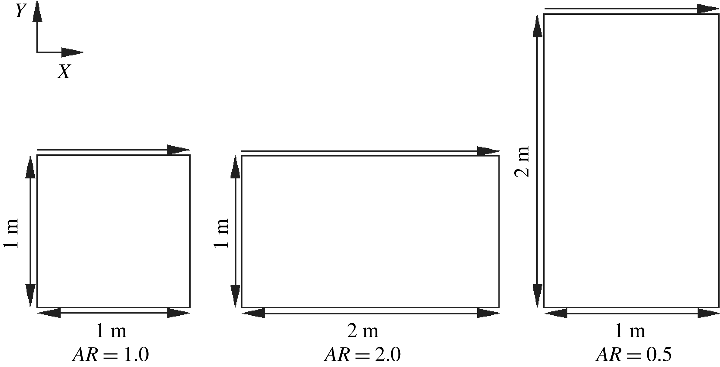
A schematic of cavities of different aspect ratios is shown in figure 1. The aspect ratio (AR) of a cavity is defined as follows:
 $$\begin{eqnarray}\displaystyle AR=\frac{\text{width of the cavity}}{\text{depth of the cavity}}. & & \displaystyle\end{eqnarray}$$
The aspect ratios of the three cavities in figure 1 are 1.0, 2.0 and 0.5. These will be referred to as the square, wide and deep cavities, respectively, in the subsequent sections. A flow is induced in the cavity by driving the top wall (lid) at different Mach numbers (
 $M_{lid}$
) defined as:
 $$\begin{eqnarray}\displaystyle M_{lid}=\frac{U_{lid}}{a};\quad a=\sqrt{\unicode[STIX]{x1D6FE}RT_{wall}}. & & \displaystyle\end{eqnarray}$$
The degree of rarefaction within the cavity is prescribed based on the reference Knudsen number,
 $Kn_{r}$
, defined as the ratio of free-stream mean free path (
 $\unicode[STIX]{x1D706}_{r}$
) to the characteristic length scale of the cavity (
 $L$
). The value of
 $\unicode[STIX]{x1D706}_{r}$
is defined based on the variable hard sphere (VHS) collision model.
 $$\begin{eqnarray}\displaystyle Kn_{r}=\frac{\unicode[STIX]{x1D706}_{r}}{L};\quad \unicode[STIX]{x1D706}_{r}(VHS)=\frac{16\unicode[STIX]{x1D707}_{r}}{5\unicode[STIX]{x1D70C}r\sqrt{2\unicode[STIX]{x03C0}RT_{r}}}=\frac{1}{\sqrt{2}\unicode[STIX]{x03C0}d_{r}^{2}n_{r}}. & & \displaystyle\end{eqnarray}$$
The subscript
 $r$
denotes the free-stream (reference) state;
 $d$
and
 $n$
are the molecular diameter and number density, respectively. At all of the walls of the cavity, a constant temperature (isothermal) of 273 K is maintained and no penetration boundary conditions are applied. The mathematical formulation of the boundary conditions in the kinetic theory framework is described in detail in Venugopal & Girimaji (Reference Venugopal and Girimaji2015), Venugopal (Reference Venugopal2016).
Dimensions of cavities with different aspect ratios.

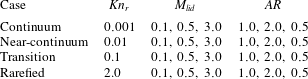
Four sets of numerical experiments are performed to span a broad range of reference Knudsen numbers (table 1). For a given
 $Kn_{r}$
, the lid Mach numbers (
 $M_{lid}$
) are chosen such that the flows can be classified into the incompressible subsonic (
 $M_{lid}=0.1$
), compressible subsonic (
 $M_{lid}=0.5$
) and supersonic (
 $M_{lid}=3.0$
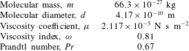
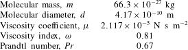
) regimes. Simulations are performed with argon gas (table 2) as the medium. Gauss–Hermite quadrature with
 $28\times 28$
discrete velocity points is utilized for simulations of low-speed, near-continuum flows. In rarefied high-speed flows, this choice of discrete velocities yields unphysical oscillations when the ordinate range is large and the minimum and maximum values of the velocity are far from the central value. This makes the contributions of the extreme velocity values to the integration negligible as the quadrature spans the entire velocity space (Guo, Xu & Wang Reference Guo, Xu and Wang2013). To overcome this limitation, we use Newton–Cotes quadrature with
 $100\times 100$
discrete velocity ordinates to capture the correct physical behaviour for high Knudsen and Mach numbers. Please see Venugopal & Girimaji (Reference Venugopal and Girimaji2015) for more details on the choice of velocity phase space discretization for different Mach and Knudsen numbers. A spatial resolution of
 $100\times 100$
, with a Courant–Friedrichs–Lewy (CFL) number of
 $0.6$
is chosen after a thorough grid sensitivity analysis.
Two sets of UGKS simulations are performed. The first set is used to examine the physical features of thermal transport in micro-cavities. The second set is performed expressly to compare the UGKS results against extended thermodynamic models. In the second part, the Prandtl number is set to unity as the augmented Burnett and the BGK-Burnett models do not account for Prandtl number effects. It is important to note that a change in the Prandtl number did not significantly affect the fundamental features of the observed thermal transport.
Due to the motion of the lid, the flow domain experiences an initial transient stage. After the transients are complete, the flow settles down to a steady or statistically steady state. Thermal transport characteristics are examined after the initial transients have subsided. The transient stage is investigated in the entropy evolution analysis. We now present the verification study results.
Simulation parameters.

Properties of argon gas at reference state (
 $101\,325$
Pa and 273 K).
4.2 Three-dimensional versus two-dimensional DSMC
Three-dimensional (3-D) DSMC computations are performed using the open source code dsmcFOAM for a cubic cavity of
 $AR=1$
. The end planes in the third direction are considered periodic and all other walls including the lid are kept at a constant temperature of 273 K. A Maxwellian diffuse reflection model is selected for representing the gas–surface interaction with the solid walls. The number of collision subcells are automatically generated by dsmcFOAM based on the free-stream number density and the number of molecules representing a simulated particle,
 $F_{num}$
. This is chosen such that there are
 $20$
simulated particles on an average per sampling cell. The time step was set to be one third of the mean collision time in the reference state
 $\unicode[STIX]{x1D70F}_{ref}$
given by:
 $$\begin{eqnarray}\displaystyle \unicode[STIX]{x1D70F}_{ref}=\frac{1}{\unicode[STIX]{x03C0}d_{ref}^{2}n_{ref}\overline{c}_{r,ref}}, & & \displaystyle\end{eqnarray}$$
where,
 $\overline{c}_{r,ref}=(16kT_{ref}/\unicode[STIX]{x03C0}m)^{1/2}$
is the mean magnitude of the relative velocity of colliding molecules in the reference state. The reference Knudsen numbers (
 $Kn_{r}$
) for the 3-D simulations are chosen to be
 $0.5$
and
 $4.0$
with lid Mach numbers of
 $0.5$
and
 $1.0$
.
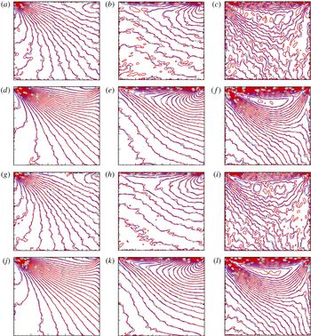
Two-dimensional DSMC (blue) versus 3-D DSMC (red). [
 $Kn_{r}$
,
 $M_{lid}$
] are as follows. (a–c) [
 $0.5$
,
 $0.5$
]; (d–f) [
 $0.5$
,
 $1.0$
]; (g–i) [
 $4.0$
,
 $0.5$
]; (j–l) [
 $4.0$
,
 $1.0$
]. (a,d,g,j): isotherms; (b,e,h,k): constant
 $q_{x}$
lines; (c,f,i,l) constant
 $q_{y}$
lines.

The temperature profiles and heat flux components at statistically steady state are compared with corresponding two-dimensional DSMC simulations as shown in figure 2. It can be seen that the peak temperature is always at the top right corner in all cases, which is captured well even with a 2-D DSMC model. The temperature contours and heat flux components within the cavity computed by 3-D and 2-D DSMC simulations match well with each other. However, the isotherms are not smooth in any of the 3-D simulations, which could be attributed to statistical noise. The velocity profiles of the 2-D DSMC cases have already been verified with the corresponding 3-D cases in Venugopal & Girimaji (Reference Venugopal and Girimaji2015). The implication is clearly that key transport features can be more expeditiously examined in a 2-D calculation as it requires a significantly lower level of computational resources.
4.3 Two-dimensional DSMC versus 2-D UGKS
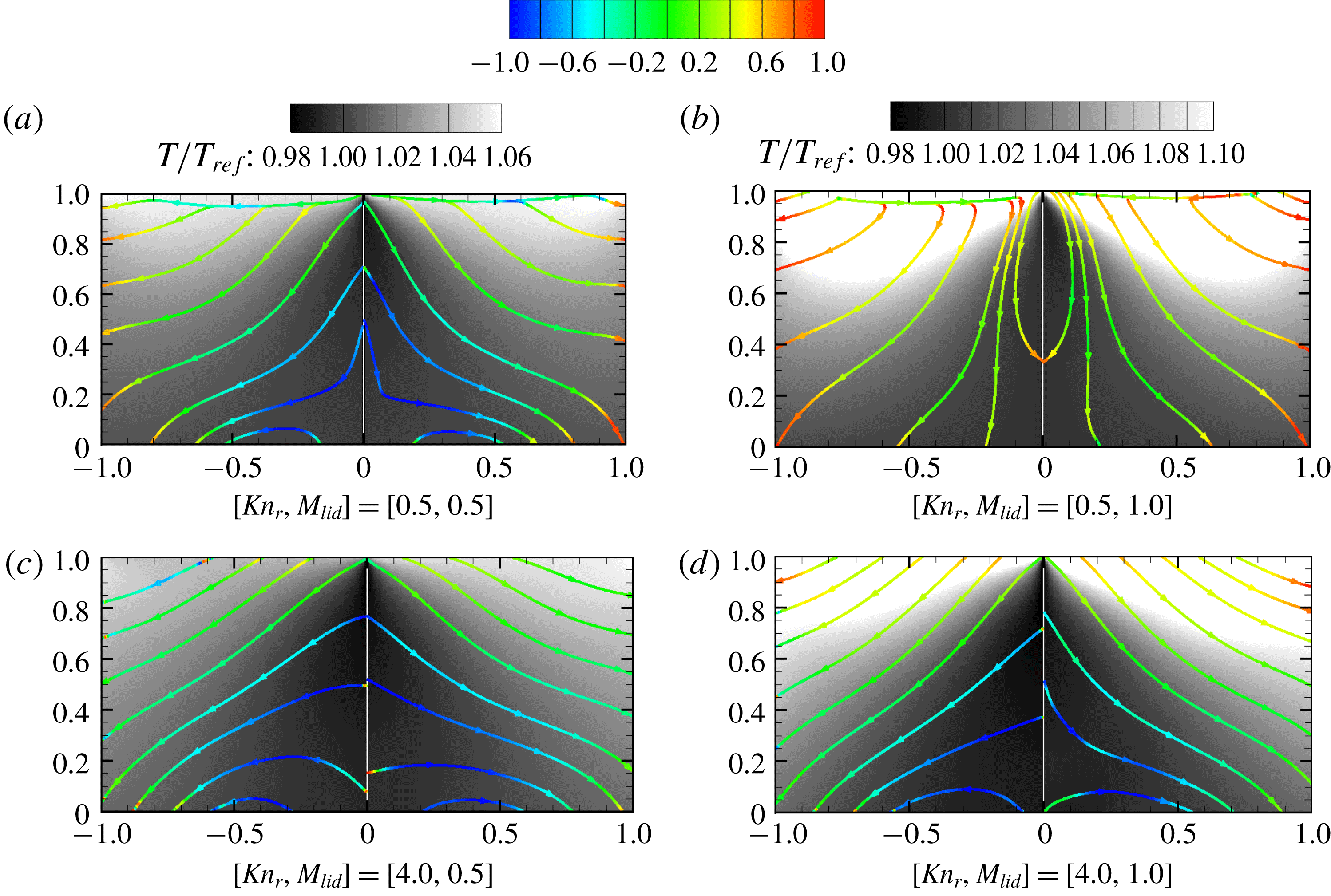
Two-dimensional UGKS simulations are now performed to verify the results against the corresponding 2-D DSMC data. The temperature contours overlaid by streamlines of heat flux are illustrated in figure 3. It can be seen that the heat flux streamlines and the temperature contours computed from the 2-D UGKS simulation agree well with its 2-D DSMC counterpart. The streamlines are coloured according to the cosine of the angle
 $\unicode[STIX]{x1D6FD}$
which is defined as the angle between the negative temperature gradient
 $(-\unicode[STIX]{x1D735}T)$
and the heat flux vector
 $(\boldsymbol{q})$
. A value of unity (red colour in figure 3) for this measure implies a counter-gradient heat flux, i.e. heat flux opposite to the temperature gradient, in conformance with the Fourier relationship. Any other value for this measure would indicate that the Fourier constitutive heat flux model is violated. The degree of violation can be surmised from the colour code of
 $\cos (\unicode[STIX]{x1D6FD})$
. It can be concluded from figure 3 that the heat flux lines violate the Fourier relationship over a large portion of the domain in the highly rarefied case (
 $Kn_{r}=4.0$
). The purpose of this comparison is to demonstrate that the 2-D UGKS and the 2-D DSMC results are qualitatively and, even more importantly, quantitatively similar.
DSMC (left half) versus UGKS (right half) comparison: temperature contours overlaid with heat flux streamlines coloured by
 $\cos (-\unicode[STIX]{x1D735}T,\boldsymbol{q})$
. The contour legend of alignment,
 $\cos (-\unicode[STIX]{x1D735}T,\boldsymbol{q})$
, is given above.

The verification studies lead to two important observations: (i) 2-D DSMC agrees very well with 3-D DSMC results for a variety of flow and thermodynamic variables; and (ii) 2-D UGKS results match well with those of 2-D DSMC for the flow configurations considered. Similar observations regarding transport properties in 2-D microcavity flows have been made by other authors – e.g. Mohammadzadeh et al. (Reference Mohammadzadeh, Roohi, Niazmand, Stefanov and Myong2012).
Computational cost. For
 $Kn_{r}<1$
, UGKS is an order of magnitude cheaper than DSMC, as it requires only
 $28\times 28$
Gauss–Hermite points in the velocity space. For
 $Kn_{r}>1$
, UGKS uses
 $100\times 100$
Newton–Cotes quadrature points for velocity–space discretization. Thus, the memory and computational requirements of UGKS are higher than those of DSMC in the rarefied regime. By utilizing implicit schemes and adaptive mesh refinement techniques, UGKS has been proven to demonstrate better performance than DSMC even in hypersonic rarefied flows over complex geometries (Zhu, Zhong & Xu Reference Zhu, Zhong and Xu2017). As this paper only focuses on the proof-of-concept of UGKS within all regimes of
 $Kn_{r}$
, we do not make attempts to reduce the computational burden.
We now proceed to perform a comprehensive study of thermal transport at different Mach and Knudsen numbers in 2-D cavity flows.
5 Results and discussion
The UGKS simulation results provide important physical insight and quantitative data for characterizing momentum and thermal transport over a wide range of Knudsen and Mach numbers. While the long term goal of the present effort is to characterize both momentum and thermal transport, the focus of this paper is restricted to thermal flux. Momentum transport is more complicated as it entails characterizing a stress tensor as opposed to a thermal flux vector. This data set will be used in future work to investigate momentum transfer as well.
Normalized temperature ranges achieved in UGKS simulations for different
 $M_{lid},Kn_{ref}$
and
 $AR$
. Ratios of maximum-to-stagnation temperatures (
 $\unicode[STIX]{x1D703}_{s}$
) are also indicated for all of the simulations.
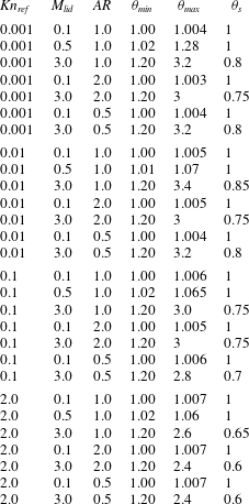
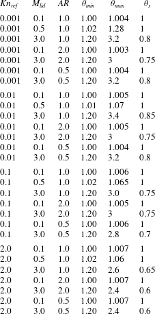
In table 3, we present the global minimum and maximum temperatures attained within the cavity as a function of Knudsen number, lid Mach number and cavity shape:
 $$\begin{eqnarray}\displaystyle \unicode[STIX]{x1D703}_{min}=\frac{T_{min}}{T_{ref}};\quad \unicode[STIX]{x1D703}_{max}=\frac{T_{max}}{T_{ref}};\quad T_{ref}=273\;\text{K}. & & \displaystyle\end{eqnarray}$$
The ratio of maximum temperature to the stagnation temperature,
 $\unicode[STIX]{x1D703}_{s}$
, is also presented:
 $$\begin{eqnarray}\displaystyle \unicode[STIX]{x1D703}_{s}=\frac{T_{max}}{T_{s}};\quad \text{where, }T_{s}\equiv T_{ref}\left(1+\frac{\unicode[STIX]{x1D6FE}-1}{2}M_{lid}^{2}\right). & & \displaystyle\end{eqnarray}$$
The difference between the minimum and maximum temperatures represents the thermal transport potential within the cavity. Stagnation temperature is a measure of the maximum temperature that can be attained within the cavity.
In all cases, the minimum cavity temperature is close to the reference or free-stream value. The maximum temperature occurs in the vicinity of the downstream upper lip (corner) of the cavity. The distributions of the temperature within the cavity depend strongly on the Knudsen and Mach numbers. This will be discussed in detail later. The attained value of maximum temperature also shows a dependence on all the three parameters – Knudsen number, Mach number and aspect ratio. The maximum temperature goes up to three times the value of the free-stream temperature at the highest Mach number. The value of
 $\unicode[STIX]{x1D703}_{s}$
decreases with Mach number. The observed behaviour is weakly dependent on aspect ratio.
At low Mach and Knudsen numbers (continuum limit),
 $\unicode[STIX]{x1D703}_{s}$
is nearly unity. Even at higher Knudsen numbers, the ratio is still close to unity so long as the Mach number remains small. In the continuum limit, the maximum-to-stagnation temperature ratio decreases with increasing Mach number and attains a value of approximately
 $0.80$
at
 $M_{lid}=3.0$
. The reduction is more pronounced when both the Knudsen and Mach numbers are high. For
 $Kn_{r}=2.0$
and
 $M_{lid}=3.0$
,
 $\unicode[STIX]{x1D703}_{s}$
value goes down to approximately
 $0.6$
. The observed behaviour can be understood by examining the number of molecular collisions required to achieve the stagnation temperature. In low Mach number flows, the stagnation temperature is not very different from the free-stream temperature due to the small value of the continuum (collective molecular) velocity. As a result, only a small number of collisions is required to attain the stagnation temperature. However, with increasing Mach number, the difference between the free-stream and stagnation energy escalates. Then substantially high number of collisions is required to transfer energy from kinetic to internal forms. In low Knudsen number flows, the frequency of the collisions is high, leading to a higher
 $\unicode[STIX]{x1D703}_{s}$
. Conversely, at higher Knudsen numbers there is a smaller number of collisions, leading to a reduced maximum-to-stagnation temperature ratio. Further, owing to the fact that the difference in the free-stream and stagnation velocities is very small at low Knudsen and Mach numbers, the temperature gradients are very mild in these simulation cases. This observation will be invoked later in the paper to explain some of the observed thermal flux behaviour.
Preliminary examination of the thermal flux data indicates that the direction, rather than the magnitude, of the flux vector shows vast deviations from the Fourier and extended thermodynamic model predictions. As will be seen shortly, the thermal flux even exhibits a co-temperature gradient, rather than the classical counter-temperature-gradient alignment, in many regions of the flow. In unforced and isolated systems, co-gradient diffusion/conduction is generally considered a violation of the second law of thermodynamics. In the present case, the system is forced by the moving lid and hence, deviations from the Fourier law can be expected. Non-classical thermal transfer has been reported in open systems of supersonic, non-equilibrium gas flows of non-uniform relaxation (Aristov Reference Aristov1998; Aristov, Frolova & Zabelok Reference Aristov, Frolova and Zabelok2009, Reference Aristov, Frolova and Zabelok2012; Ilyin Reference Ilyin2017).
Motivated by the preliminary findings, we focus on thermal transport alignment and entropy analyses.
5.1 Thermal transport alignment
The thermal flux behaviour is investigated in the continuum, near-continuum, transition and rarefied cavity regimes whose reference Knudsen numbers are
 $0.001$
,
 $0.01$
,
 $0.1$
and
 $2$
respectively. Thermal flux vectors are calculated from UGKS simulations and the orientation is compared against the flux vectors computed using the Fourier, augmented Burnett and BGK-Burnett constitutive models. At any given point in space, the cosine of the angle between the UGKS and model flux vectors is taken to be the local measure of deviation or error in the constitutive relation. For example,
 $\cos (Q_{UGKS},Q_{AB})$
would be the deviation measure of the augmented Burnett heat flux (
 $Q_{AB}$
) with respect to the UGKS field. These deviations are characterized for each
 $Kn_{r}$
,
 $M_{lid}$
and
 $AR$
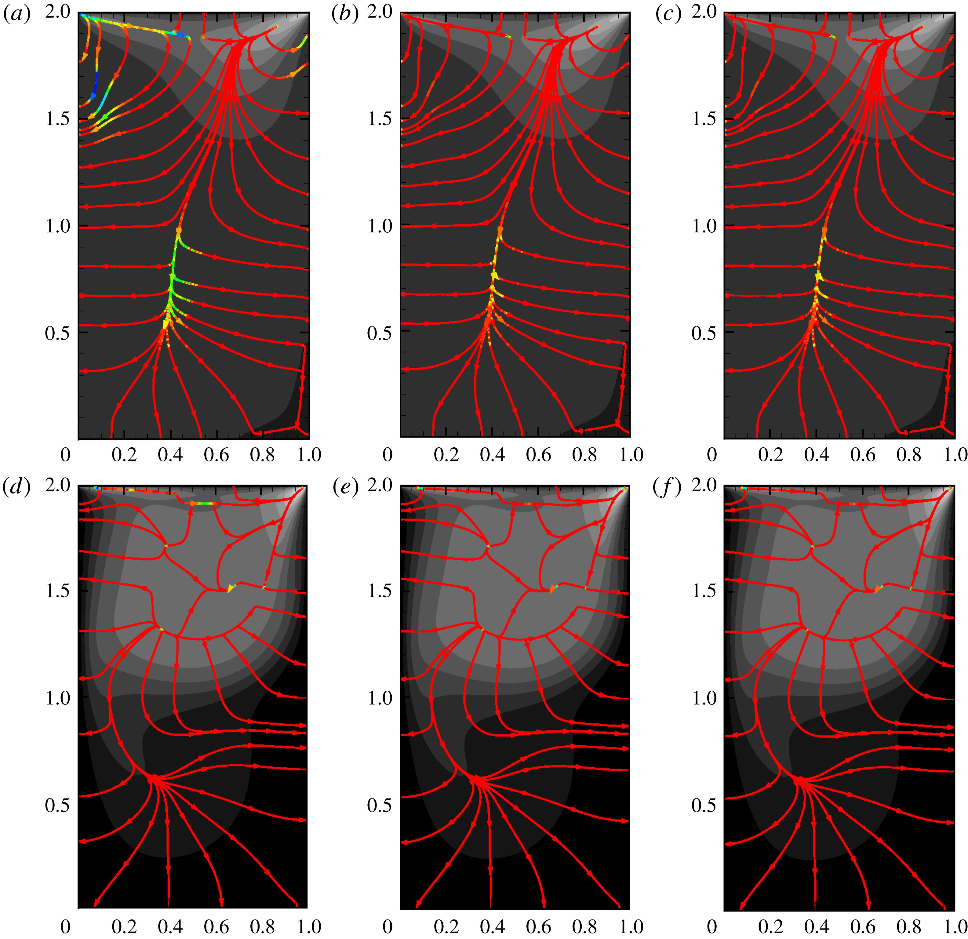
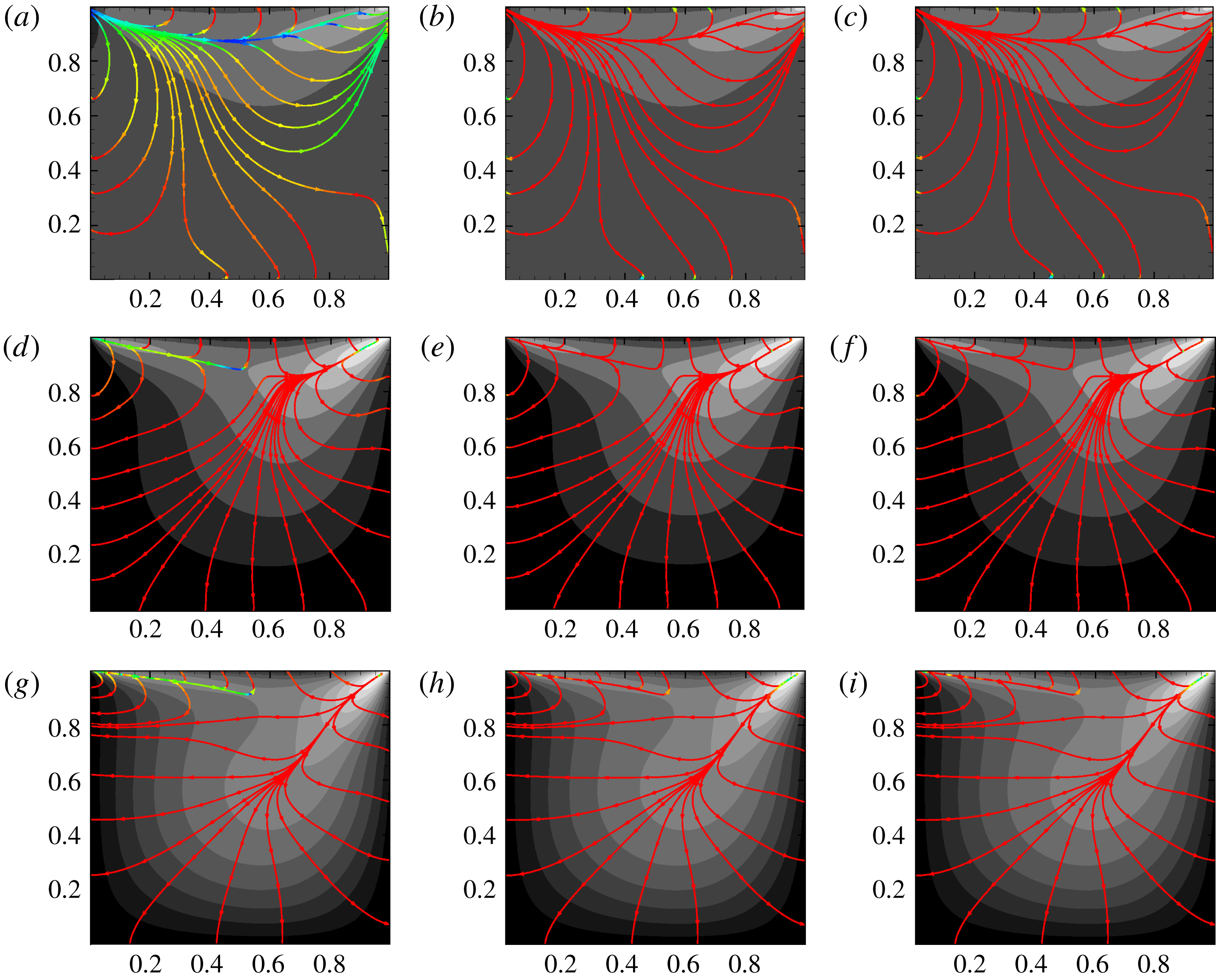
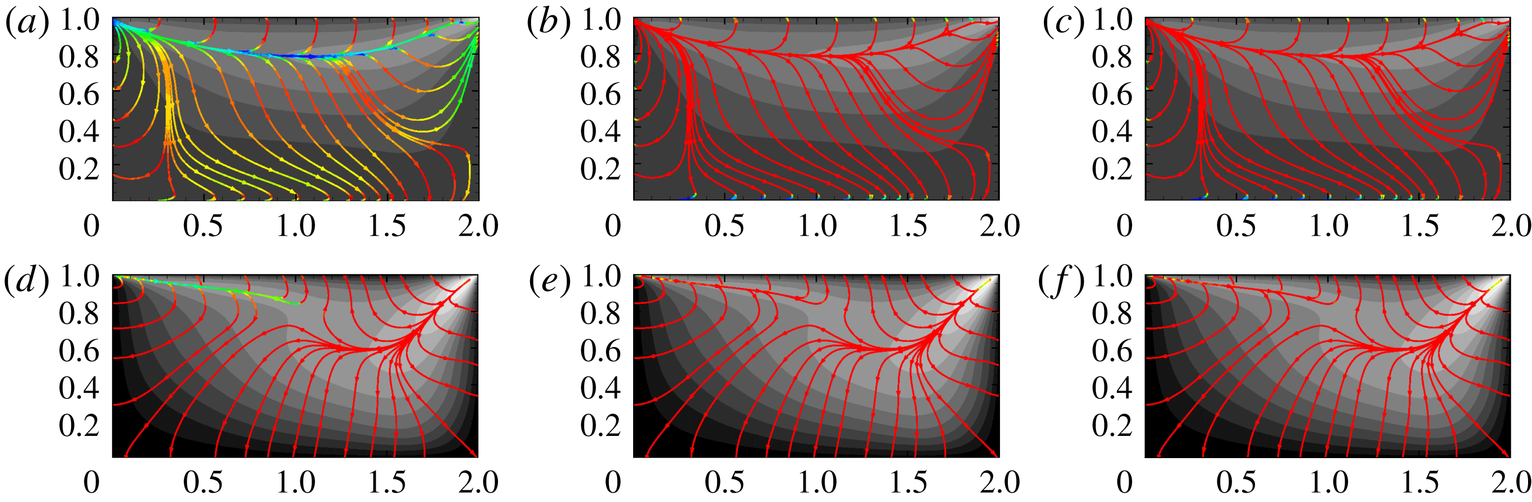
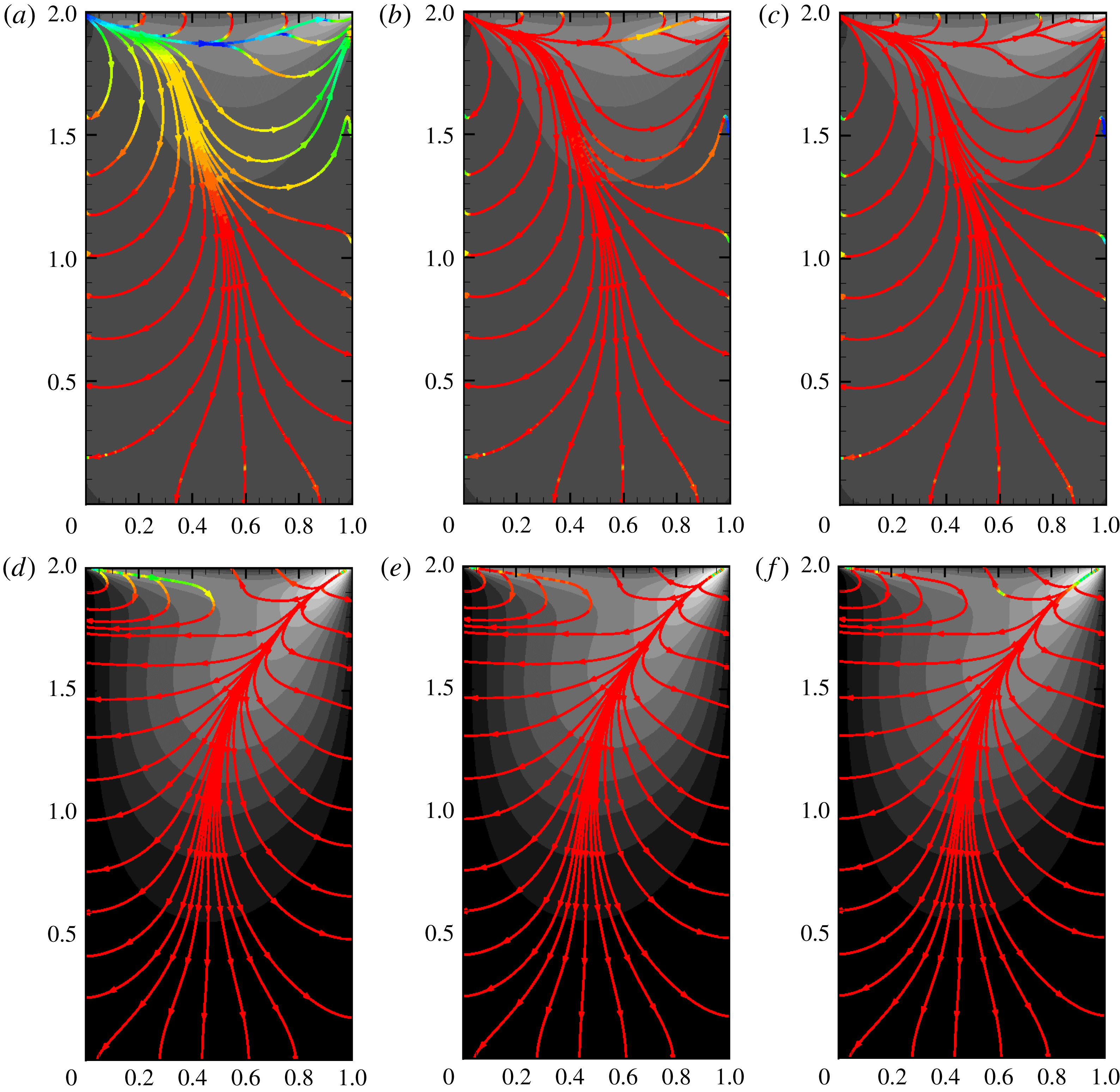
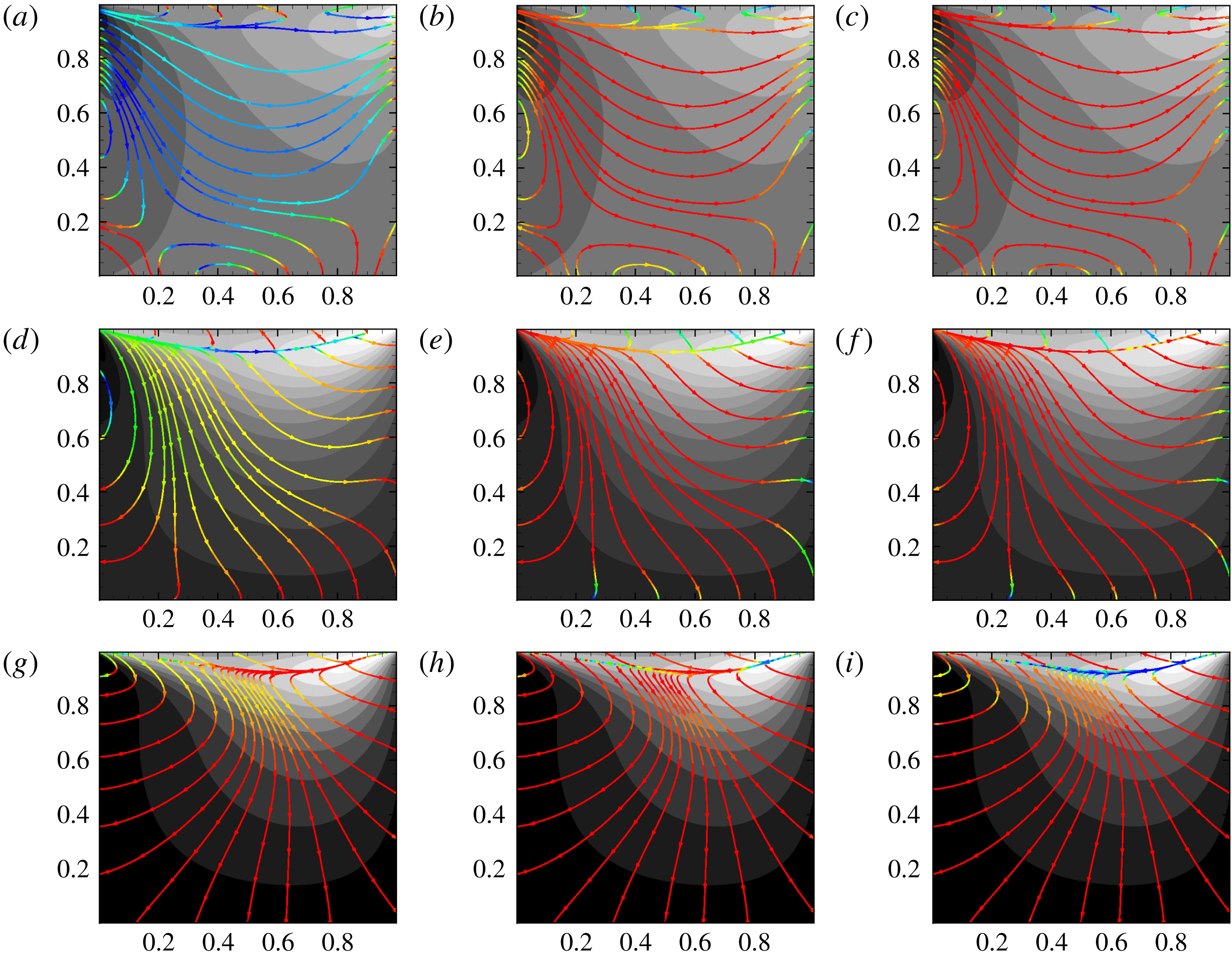
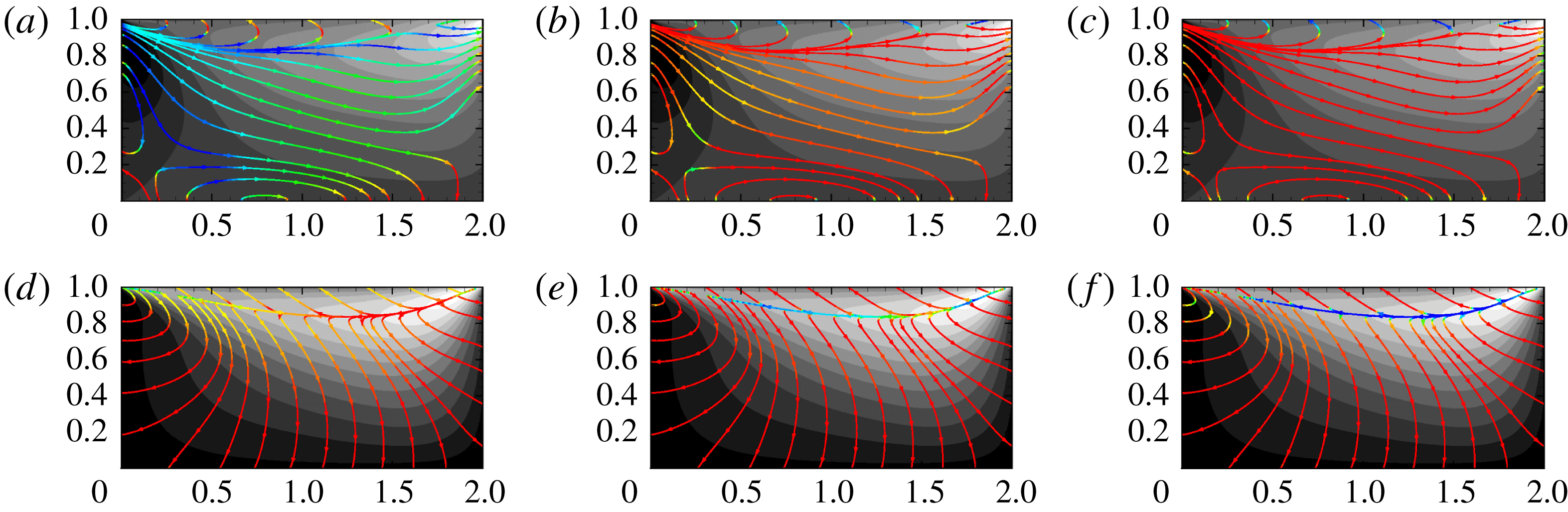
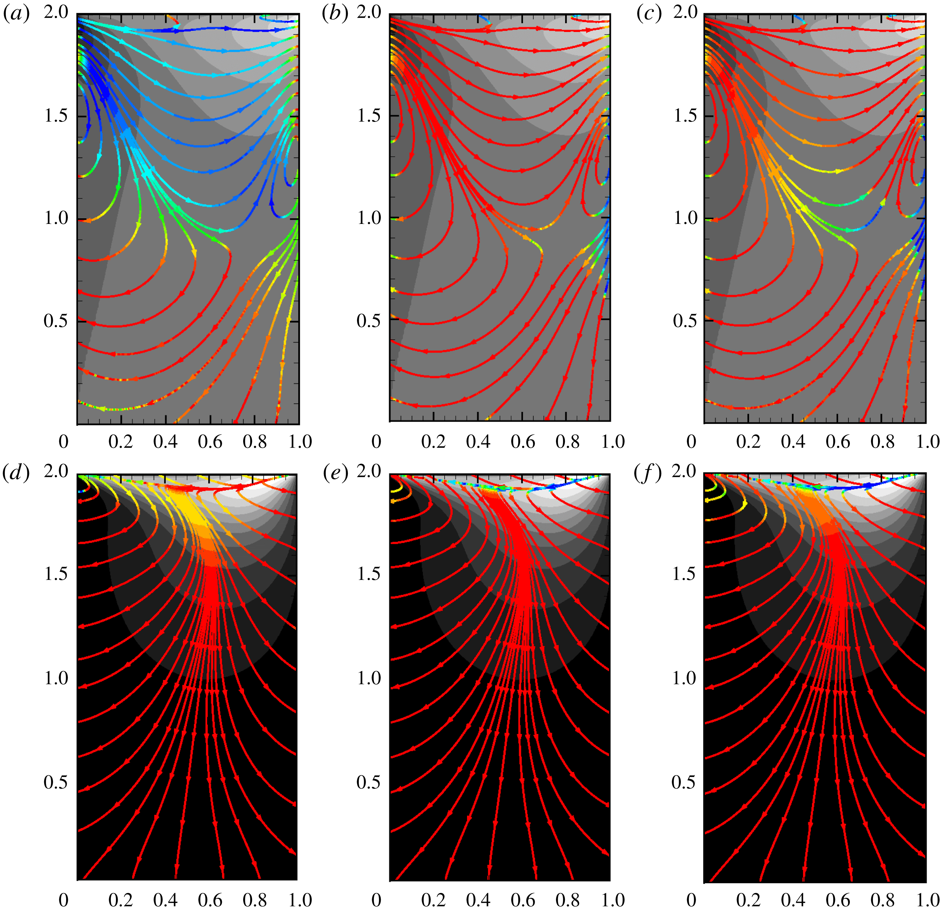
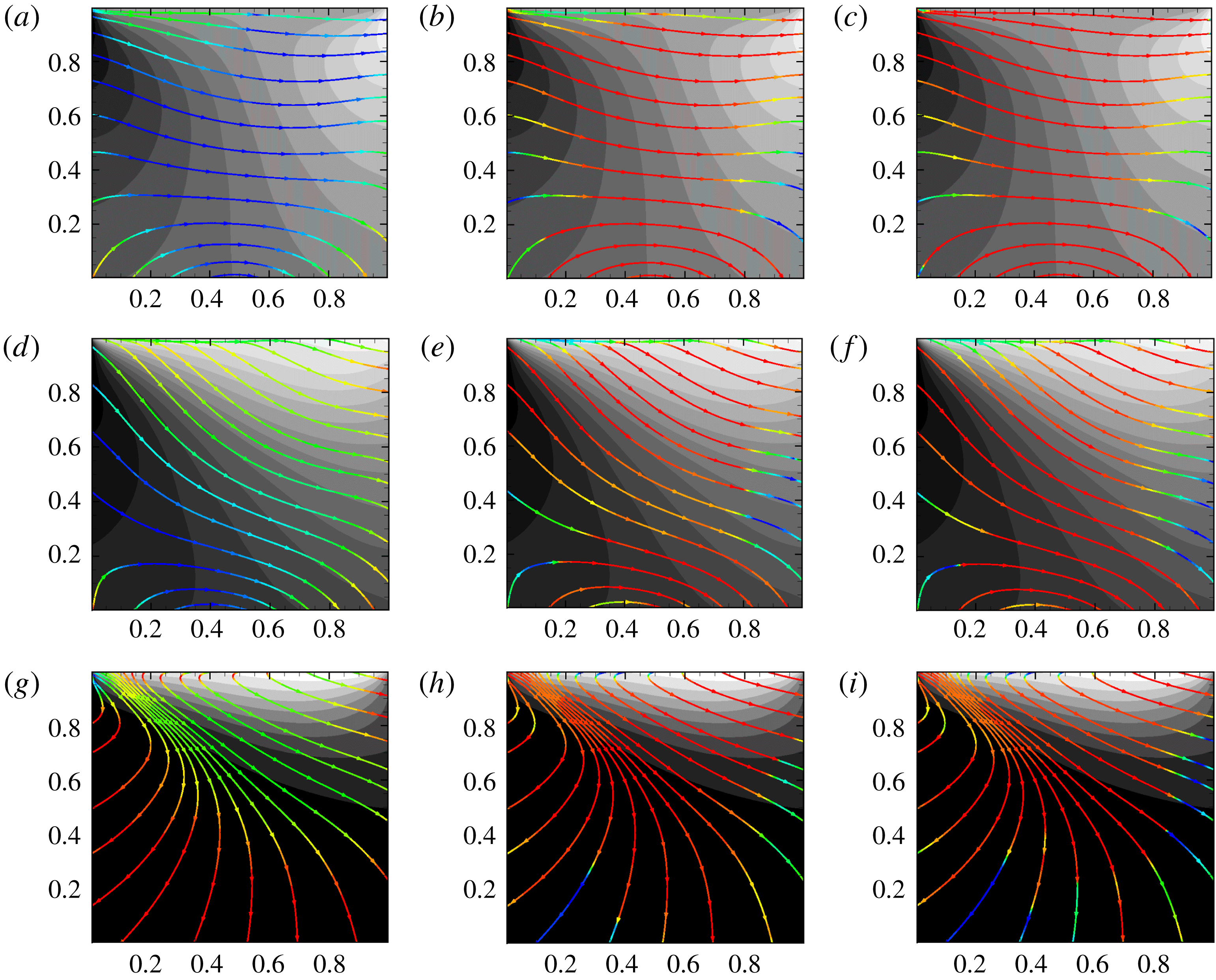
in figures 4–15. The figures show temperature (grey scale) contours overlaid by the heat flux streamlines of the corresponding cases. It is very important to note that the temperature levels in each plot are different. The maximum (white or light grey) and minimum (black) temperatures for each figure are as given in table 3. The heat flux streamlines are coloured according to the local deviation measure – i.e. the cosine of the angle between the UGKS and the constitutive relation under consideration. A value of
 $+1$
(red) for this measure would then imply that the modelled flux is in agreement with the corresponding UGKS flux. On the other hand, a value of
 $-1$
(blue) indicates that the UGKS and model fluxes are in exactly opposite directions, indicating maximum disagreement between the two. Red colouring of the Fourier flux line indicates classical counter-gradient thermal transport. On the other hand, blue coloured lines represent local co-gradient thermal flux. Yellow and green colours indicate intermediate degrees of violation.
The results are presented in four groupings based on the reference Knudsen number. In each group, the first set of figures shows the results for square cavities with
 $AR=1.0$
, the second set for wide cavities of
 $AR=2.0$
and the third set for deep cavities of
 $AR=0.5$
. As mentioned earlier, for each Knudsen number, we consider three different Mach numbers ranging from subsonic to supersonic. All three speeds are illustrated for square cavities, whereas for the other shapes, only the extreme speeds are discussed.
5.1.1 Continuum regime (
 $Kn_{r}=0.001$
)

Temperature contours and flux alignment deviation measures (cosine of angles) in the continuum flow cavity (
 $Kn_{r}=0.001$
) are shown in figures 4–6 for cavity aspect ratios of
 $1$
,
 $2$
and
 $0.5$
respectively.
For the low Mach number case of
 $M_{lid}=0.1$
(a–c of figures 4–6), the maximum temperature within the cavity is only approximately
 $0.5\,\%$
higher than the lowest temperature. At low
 $M_{lid}$
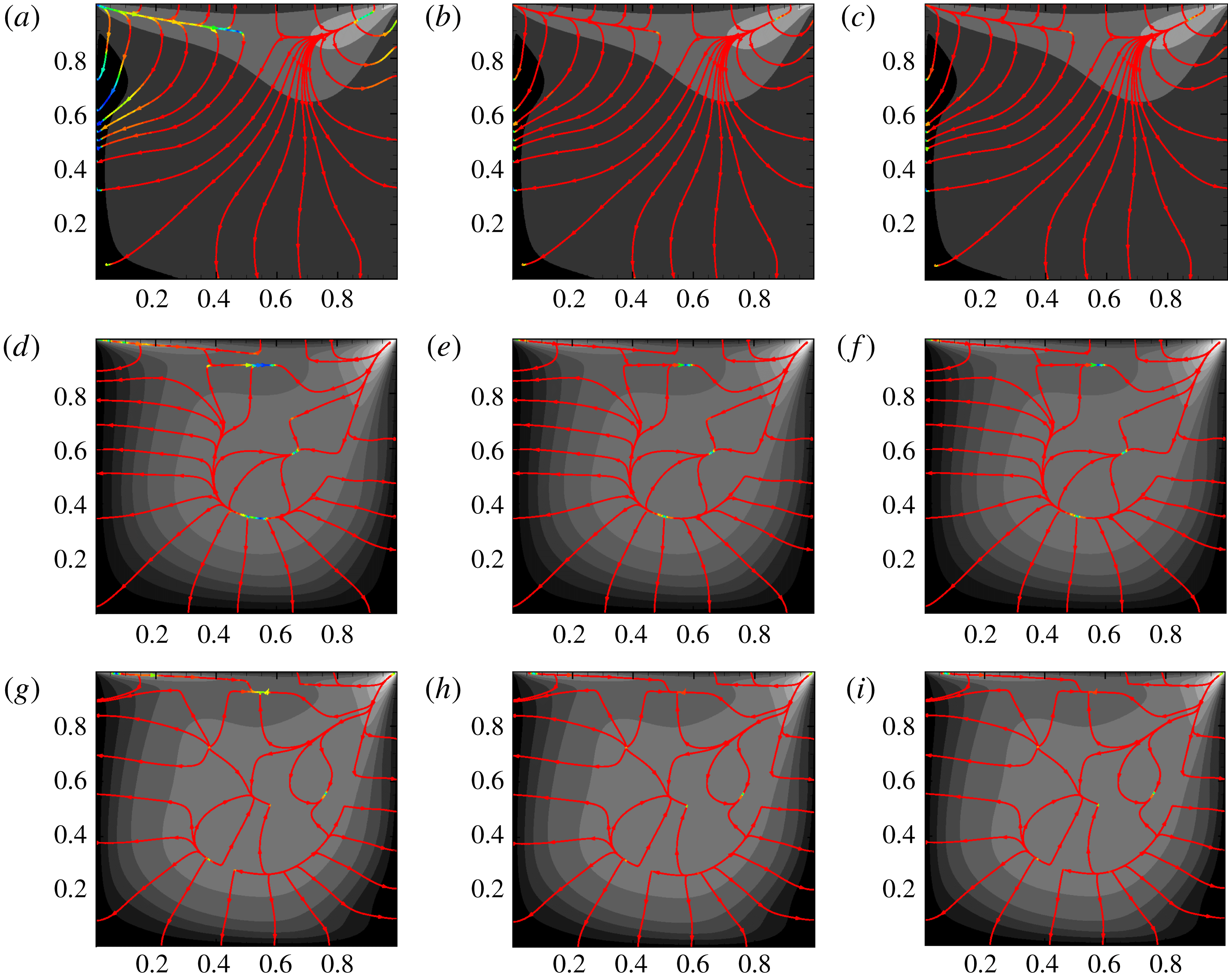
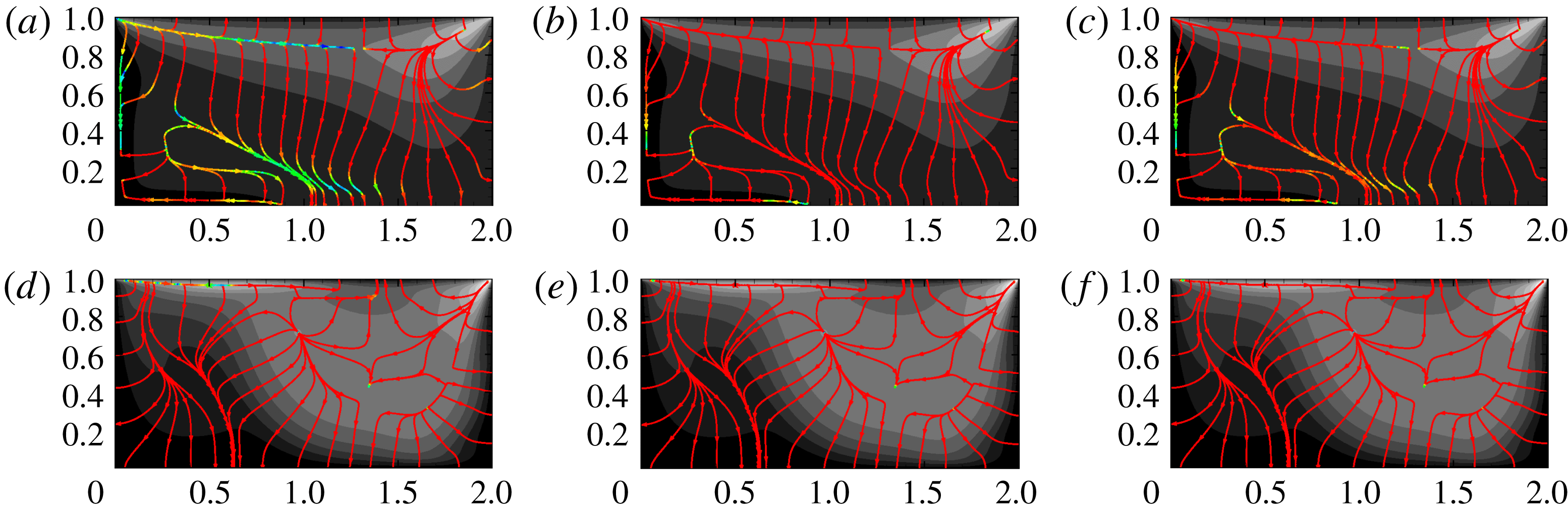
, higher temperatures are restricted to the top of the cavity. The thermal fluxes throughout the cavity are very small. It can be seen that the Fourier heat flux model (a) alignment is inaccurate in a region of the domain for all of the cavity aspect ratios. Due to the vanishingly small temperature gradients in this region, the first-order Fourier model cannot represent the thermal flux computed from the kinetic simulation accurately. However, it must be noted that the Fourier model error is quite small in terms of heat flux magnitude. The augmented Burnett and BGK-Burnett (b,c) models are in good agreement with UGKS flux alignments. In the absence of the first derivative of the temperature, the heat flux is governed exclusively by higher-order terms in the expansion. The extended thermodynamic models with higher-order terms easily capture the heat flux behaviour.
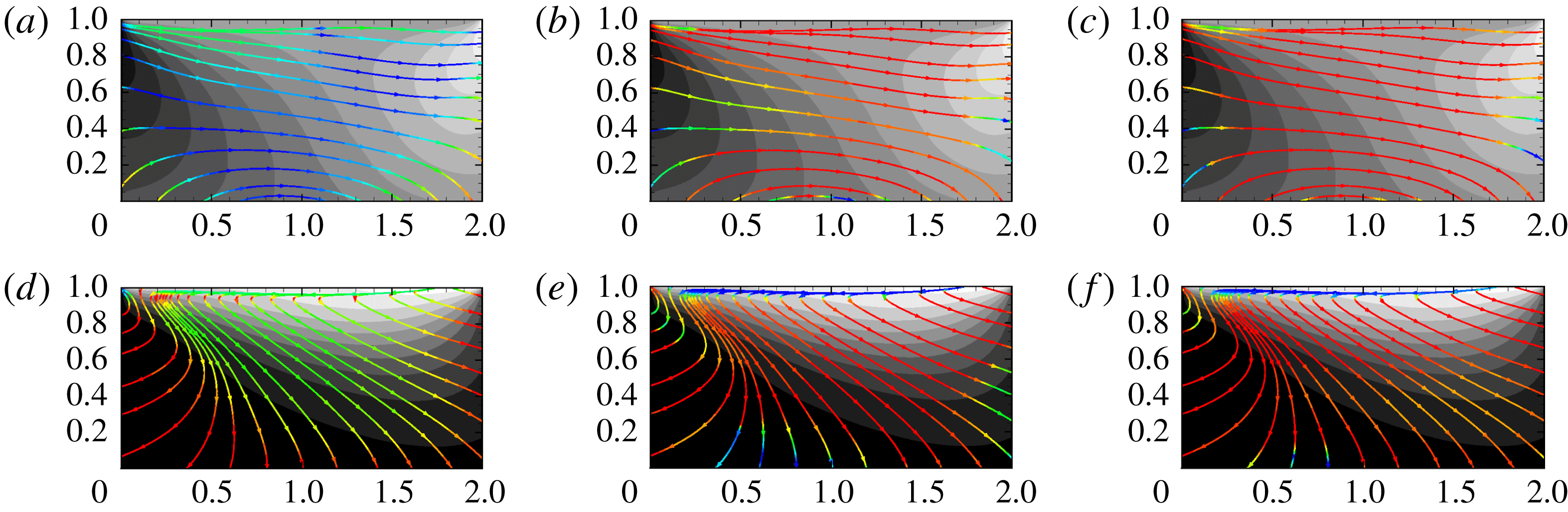
Temperature contours overlaid with heat flux streamlines for
 $Kn_{r}=0.001$
,
 $AR=1.0$
. (a–c)
 $M_{lid}=0.1$
with
 $\unicode[STIX]{x1D703}_{min}=1.0$
,
 $\unicode[STIX]{x1D703}_{max}=1.004$
; (d–f)
 $M_{lid}=0.5$
with
 $\unicode[STIX]{x1D703}_{min}=1.02$
,
 $\unicode[STIX]{x1D703}_{max}=1.28$
; (g–i)
 $M_{lid}=3.0$
with
 $\unicode[STIX]{x1D703}_{min}=1.2$
,
 $\unicode[STIX]{x1D703}_{max}=3.2$
. Heat flux contours are coloured according to alignment (see figure 3 for colour scale). (a,d,g)
 $\cos (Q_{UGKS},Q_{F})$
; (b,e,h)
 $\cos (Q_{UGKS},Q_{AB})$
; and (c,f,i)
 $\cos (Q_{UGKS},Q_{BGKB})$
.

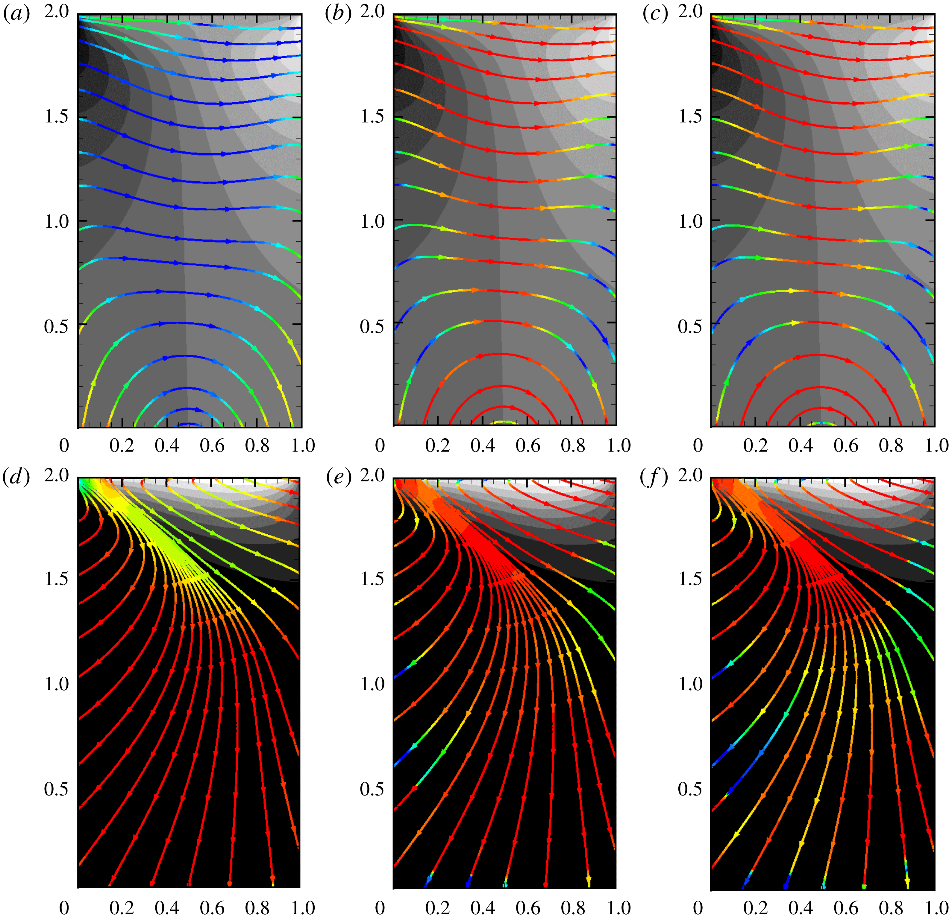
Temperature contours overlaid with heat flux streamlines for
 $Kn_{r}=0.001$
,
 $AR=2.0$
. (a–c)
 $M_{lid}=0.1$
with
 $\unicode[STIX]{x1D703}_{min}=1.0$
,
 $\unicode[STIX]{x1D703}_{max}=1.003$
; (d–f)
 $M_{lid}=3.0$
with
 $\unicode[STIX]{x1D703}_{min}=1.2$
,
 $\unicode[STIX]{x1D703}_{max}=3.0$
. Heat flux contours are coloured according to alignment (see figure 3 for colour scale). (a,d)
 $\cos (Q_{UGKS},Q_{F})$
; (b,e)
 $\cos (Q_{UGKS},Q_{AB})$
; and (c,f)
 $\cos (Q_{UGKS},Q_{BGKB})$
.

Temperature contours overlaid with heat flux streamlines for
 $Kn_{r}=0.001$
,
 $AR=0.5$
. (a–c)
 $M_{lid}=0.1$
with
 $\unicode[STIX]{x1D703}_{min}=1.0$
,
 $\unicode[STIX]{x1D703}_{max}=1.004$
; (d–f)
 $M_{lid}=3.0$
with
 $\unicode[STIX]{x1D703}_{min}=1.2$
,
 $\unicode[STIX]{x1D703}_{max}=3.2$
. Heat flux contours are coloured according to alignment (see figure 3 for colour scale). (a,d)
 $\cos (Q_{UGKS},Q_{F})$
; (b,e)
 $\cos (Q_{UGKS},Q_{AB})$
; and (c,f)
 $\cos (Q_{UGKS},Q_{BGKB})$
.

Temperature contours overlaid with heat flux streamlines for
 $Kn_{r}=0.01$
,
 $AR=1.0$
. (a–c)
 $M_{lid}=0.1$
with
 $\unicode[STIX]{x1D703}_{min}=1.0$
,
 $\unicode[STIX]{x1D703}_{max}=1.005$
; (d–f)
 $M_{lid}=0.5$
with
 $\unicode[STIX]{x1D703}_{min}=1.01$
,
 $\unicode[STIX]{x1D703}_{max}=1.07$
; (g–i)
 $M_{lid}=3.0$
with
 $\unicode[STIX]{x1D703}_{min}=1.2$
,
 $\unicode[STIX]{x1D703}_{max}=3.4$
. Heat flux contours are coloured according to alignment (see figure 3 for colour scale). (a,d,g)
 $\cos (Q_{UGKS},Q_{F})$
; (b,e,h)
 $\cos (Q_{UGKS},Q_{AB})$
; and (c,f,i)
 $\cos (Q_{UGKS},Q_{BGKB})$
.

Temperature contours overlaid with heat flux streamlines for
 $Kn_{r}=0.01$
,
 $AR=2.0$
. (a–c)
 $M_{lid}=0.1$
with
 $\unicode[STIX]{x1D703}_{min}=1.0$
,
 $\unicode[STIX]{x1D703}_{max}=1.005$
; (d–f)
 $M_{lid}=3.0$
with
 $\unicode[STIX]{x1D703}_{min}=1.2$
,
 $\unicode[STIX]{x1D703}_{max}=3.0$
. Heat flux contours are coloured according to alignment (see figure 3 for colour scale). (a,d)
 $\cos (Q_{UGKS},Q_{F})$
; (b,e)
 $\cos (Q_{UGKS},Q_{AB})$
; and (c,f)
 $\cos (Q_{UGKS},Q_{BGKB})$
.

Temperature contours overlaid with heat flux streamlines for
 $Kn_{r}=0.01$
,
 $AR=0.5$
. (a–c)
 $M_{lid}=0.1$
with
 $\unicode[STIX]{x1D703}_{min}=1.0$
,
 $\unicode[STIX]{x1D703}_{max}=1.004$
; (d–f)
 $M_{lid}=3.0$
with
 $\unicode[STIX]{x1D703}_{min}=1.2$
,
 $\unicode[STIX]{x1D703}_{max}=3.2$
. Heat flux contours are coloured according to alignment (see figure 3 for colour scale). (a,d)
 $\cos (Q_{UGKS},Q_{F})$
; (b,e)
 $\cos (Q_{UGKS},Q_{AB})$
; and (c,f)
 $\cos (Q_{UGKS},Q_{BGKB})$
.

Temperature contours overlaid with heat flux streamlines for
 $Kn_{r}=0.1$
,
 $AR=1.0$
. (a–c)
 $M_{lid}=0.1$
with
 $\unicode[STIX]{x1D703}_{min}=1.0$
,
 $\unicode[STIX]{x1D703}_{max}=1.006$
; (d–f)
 $M_{lid}=0.5$
with
 $\unicode[STIX]{x1D703}_{min}=1.02$
,
 $\unicode[STIX]{x1D703}_{max}=1.065$
; (g–i)
 $M_{lid}=3.0$
with
 $\unicode[STIX]{x1D703}_{min}=1.2$
,
 $\unicode[STIX]{x1D703}_{max}=3.0$
. Heat flux contours are coloured according to alignment (see figure 3 for colour scale). (a,d,g):
 $\cos (Q_{UGKS},Q_{F})$
; (b,e,h)
 $\cos (Q_{UGKS},Q_{AB})$
; and (c,f,i)
 $\cos (Q_{UGKS},Q_{BGKB})$
.

Temperature contours overlaid with heat flux streamlines for
 $Kn_{r}=0.1$
,
 $AR=2.0$
. (a–c)
 $M_{lid}=0.1$
with
 $\unicode[STIX]{x1D703}_{min}=1.0$
,
 $\unicode[STIX]{x1D703}_{max}=1.005$
; (d–f)
 $M_{lid}=3.0$
with
 $\unicode[STIX]{x1D703}_{min}=1.2$
,
 $\unicode[STIX]{x1D703}_{max}=3.0$
. Heat flux contours are coloured according to alignment (see figure 3 for colour scale). (a,d)
 $\cos (Q_{UGKS},Q_{F})$
; (b,e)
 $\cos (Q_{UGKS},Q_{AB})$
; and (c,f)
 $\cos (Q_{UGKS},Q_{BGKB})$
.

Temperature contours overlaid with heat flux streamlines for
 $Kn_{r}=0.1$
,
 $AR=0.5$
. (a–c)
 $M_{lid}=0.1$
with
 $\unicode[STIX]{x1D703}_{min}=1.0$
,
 $\unicode[STIX]{x1D703}_{max}=1.006$
; (d–f)
 $M_{lid}=3.0$
with
 $\unicode[STIX]{x1D703}_{min}=1.2$
,
 $\unicode[STIX]{x1D703}_{max}=2.8$
. Heat flux contours are coloured according to alignment (see figure 3 for colour scale). (a,d)
 $\cos (Q_{UGKS},Q_{F})$
; (b,e)
 $\cos (Q_{UGKS},Q_{AB})$
; and (c,f)
 $\cos (Q_{UGKS},Q_{BGKB})$
.

Temperature contours overlaid with heat flux streamlines for
 $Kn_{r}=2.0$
,
 $AR=1.0$
. (a–c)
 $M_{lid}=0.1$
with
 $\unicode[STIX]{x1D703}_{min}=1.0$
,
 $\unicode[STIX]{x1D703}_{max}=1.007$
; (d–f)
 $M_{lid}=0.5$
with
 $\unicode[STIX]{x1D703}_{min}=1.02$
,
 $\unicode[STIX]{x1D703}_{max}=1.06$
; (g–i)
 $M_{lid}=3.0$
with
 $\unicode[STIX]{x1D703}_{min}=1.2$
,
 $\unicode[STIX]{x1D703}_{max}=2.6$
. Heat flux contours are coloured according to alignment (see figure 3 for colour scale). (a,d,g)
 $\cos (Q_{UGKS},Q_{F})$
; (b,e,h)
 $\cos (Q_{UGKS},Q_{AB})$
; and (c,f,i)
 $\cos (Q_{UGKS},Q_{BGKB})$
.

Temperature contours overlaid with heat flux streamlines for
 $Kn_{r}=2.0$
,
 $AR=2.0$
. (a–c)
 $M_{lid}=0.1$
with
 $\unicode[STIX]{x1D703}_{min}=1.0$
,
 $\unicode[STIX]{x1D703}_{max}=1.007$
; (d–f)
 $M_{lid}=3.0$
with
 $\unicode[STIX]{x1D703}_{min}=1.2$
,
 $\unicode[STIX]{x1D703}_{max}=2.4$
. Heat flux contours are coloured according to alignment (see figure 3 for colour scale). (a,d)
 $\cos (Q_{UGKS},Q_{F})$
; (b,e)
 $\cos (Q_{UGKS},Q_{AB})$
; and (c,f)
 $\cos (Q_{UGKS},Q_{BGKB})$
.

Temperature contours overlaid with heat flux streamlines for
 $Kn_{r}=2.0$
,
 $AR=0.5$
. (a–c)
 $M_{lid}=0.1$
with
 $\unicode[STIX]{x1D703}_{min}=1.0$
,
 $\unicode[STIX]{x1D703}_{max}=1.007$
; (d–f)
 $M_{lid}=3.0$
with
 $\unicode[STIX]{x1D703}_{min}=1.2$
,
 $\unicode[STIX]{x1D703}_{max}=2.4$
. Heat flux contours are coloured according to alignment (see figure 3 for colour scale). (a,d)
 $\cos (Q_{UGKS},Q_{F})$
; (b,e)
 $\cos (Q_{UGKS},Q_{AB})$
; and (c,f)
 $\cos (Q_{UGKS},Q_{BGKB})$
.

For higher Mach number cases (figures 4
d–i, 5
d–f and 6
d–f) higher temperatures penetrate into larger regions of the interior. All of the three heat flux models show conformance with the UGKS heat flux. It can be seen that the maximum temperature change in the domain is much higher (
 ${\approx}300\,\%$
for
 $M_{lid}=3.0$
) than that of
 $M_{lid}=0.1$
case. Correspondingly the temperature gradients and heat flux values are large. Then the Fourier law adequately represents the heat flux. The higher-order improvements in the extended thermodynamic models are negligible.
5.1.2 Near-continuum regime (
$Kn_{r}=0.01$
)

Results for the near-continuum regime (
 $Kn_{r}=0.01$
) square, wide and deep cavity cases are shown in figures 7, 8 and 9, respectively.
For the low Mach number (
 $M_{lid}=0.1$
) case shown in (a) of figures 7–9, it can be seen that the violations of the Fourier models at low temperature gradients are far more pronounced. The inaccuracy of the Fourier heat flux model extends deeper into all the three cavities as compared to the continuum case. However, the Fourier model is still reasonable towards the bottom of the square (figure 7
a) and deep (figure 9
a) cavities. Consistent with the behaviour exhibited at
 $Kn=0.001$
, the augmented Burnett and BGK-Burnett (b,c) capture the UGKS heat flux accurately at lower speeds.
The behaviour of the Fourier heat flux is improved as the Mach number increases (figures 7 d,g, 8 d and 9 d). However, the Fourier heat flux still does not capture the physics accurately near the lid. This is due to fact that particles accumulate deep in the cavity as they are trapped in a recirculation region. This accumulation creates continuum-like conditions locally at the bottom of the cavity, even though the top of the cavity continues to experience high Knudsen number effects. As before, the augmented Burnett (figures 7 e,h, 8 e and 9 e) and BGK-Burnett (figures 7 f,i, 8 f and 9 f) models capture the heat fluxes accurately for all of the Mach numbers and cavity geometries.
5.1.3 Transition regime (
$Kn_{r}=0.1$
)

Figures 10–12 illustrate the results when the reference Knudsen number is
 $0.1$
, a value that is typical of the transition regime.
At low Mach numbers, a distinct change in the temperature distribution within the cavity is observed. The high temperature regions shift from the cavity centre toward the downstream wall. This is due to the reduced number of collisions in the interior at higher Knudsen numbers. The collisions with the walls are not affected by the Knudsen number. As shown in figure 10 (a), it can be seen that the Fourier model is inaccurate nearly everywhere. Indeed co-gradient transport is observed at the central region of the cavity. Similar observations can be made even for the wide cavity case at low Mach number (figure 11 a). However, for a deep cavity (figure 12 a), the Fourier law is upheld in the bottom half of the cavity. This, once again, is due to the accumulation of particles deep in the recirculation region of the cavity, resulting in local continuum conditions. Extended thermodynamic model fluxes (b,c) on the other hand predict the heat flux accurately in the interior, but poorly near the boundaries. The near-wall violation can perhaps be attributed to significant temperature and velocity slip, i.e. significant differences in the properties of the molecules and the wall, at this degree of rarefaction.
As the lid Mach number is increased for all the cavity geometries, a clear demarcation of the domain into locally rarefied (at the top) and continuum (at the bottom) regions can be made. This is again due to higher density of particles in the lower parts of the cavity due to the formation of a recirculating region. The domain over which Fourier law is upheld increases. The augmented Burnett and BGK-Burnett models also perform better for higher
 $M_{lid}$
as compared to the
 $M_{lid}=0.1$
case. But, the extended thermodynamic models continue to be deficient at the walls. Clearly, these models require further analysis to account for the non-equilibrium effects due to the temperature jump and velocity slip at the wall. Overall, the BGK-Burnett model performs better than the augmented Burnett model at low
 $M_{lid}$
. The converse is true at higher
 $M_{lid}$
.
5.1.4 Rarefied regime (
$Kn_{r}=2.0$
)

The fully rarefied flow (
 $Kn_{r}=2.0$
) results for square, wide and deep cavities are shown in figures 13–15, respectively. The temperature distribution within the cavity changes further. At lower Mach numbers, the high temperature region shifts completely to the downstream cavity wall. The recirculation region continues to be strong in the lower regions at high
 $M_{lid}$
. It can be seen that the non-equilibrium effects permeate over a larger portion of the domain as compared to what is seen in the transition regime.
For the low Mach number case of
 $M_{lid}=0.1$
, the Fourier model fails to capture the heat flux throughout the domain for all of the cavity shapes. Indeed, a co-gradient thermal flux is strongly in evidence. The underlying physics can be explained as follows. As noted earlier, in this case the downstream wall is the hottest region within the cavity. The interior temperature monotonically goes from cold upstream to hot downstream walls as the intermolecular collisions in the interior diminish in frequency. The particle (molecular) motion is nearly ballistic as it collides predominantly with the wall rather than with other molecules. This leads to thermal transport from the cold upstream wall to the hot downstream wall. The augmented Burnett and BGK-Burnett models capture the rarefaction effects everywhere in the domain except at the boundaries as in the transition regime (
 $Kn_{r}=0.1$
) cases. Even for the intermediate Mach number case (
 $M_{lid}=0.5$
for the square cavity), the performance of the Fourier model improves only marginally. The augmented Burnett and BGK-Burnett models also fail to capture the fluxes at the boundaries for the intermediate lid Mach number,
 $M_{lid}=0.5$
. For the highest Mach number (
 $M_{lid}=3.0$
) case, Fourier model captures the heat flux well in the lower half of the domain reasonably well for all cavity shapes. For this high Mach number case, the deficiency of the augmented Burnett and BGK-Burnett models spreads to the interior of the domain from the boundaries. The deficiency of higher-order Burnett models in the wall region and the consequent effects on the interior domain is more evident in the shallow cavity (figure 14) than the deep cavity (figure 15). Once again, the BGK-Burnett model is better at low
 $M_{lid}$
and the augmented Burnett is superior at higher
 $M_{lid}$
.
5.2 Entropy analysis
A precise entropy analysis of the UGKS thermal transport within the cavity is rendered difficult due to many factors. First and foremost, energy is continuously added into the system by the moving lid. However, this addition is uniform in time. In the following computation, the wall conditions are set to adiabatic to ensure further isolation of the system from the surroundings. The inhomogeneity of the flow would entail that we examine the global entropy of the cavity system. The aim of this analysis is to investigate the behaviour of the entropy as defined by the Sackur–Tetrode entropy formulation and Boltzmann
 $H$
-theorem (discussed in § 3.1). Of particular interest is the rarefied case wherein co-gradient transport is dominant.
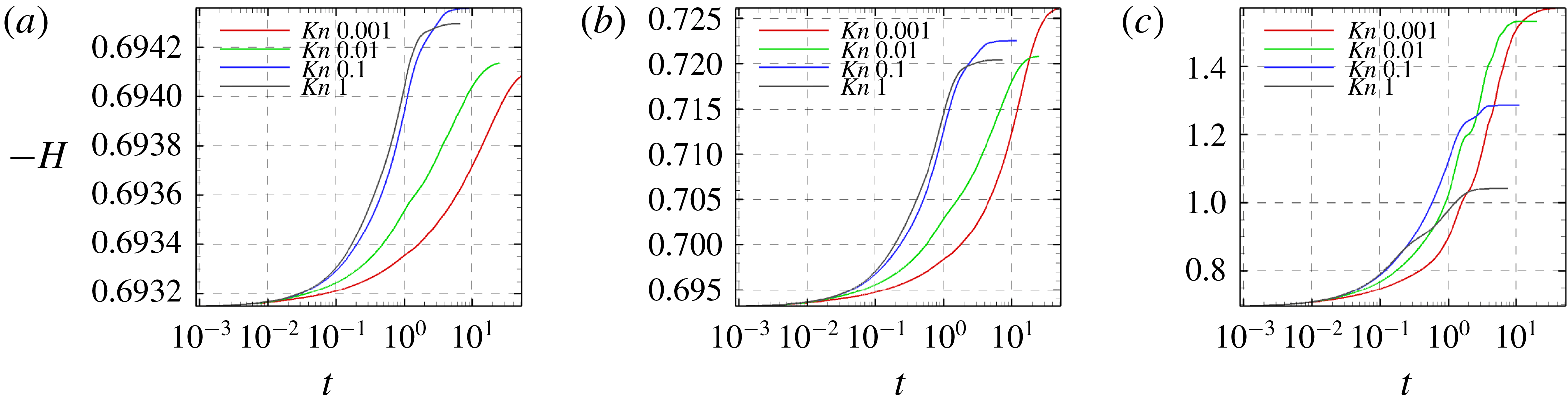
We analyse the temporal evolution of the Sackur–Tetrode entropy (
 $S_{tr}$
) and kinetic (
 $H$
)-function entropy in the cavity flow at different lid Mach (
 $M_{lid}$
) and reference Knudsen numbers (
 $Kn_{r}$
). Figure 16 compares the evolution of
 $S_{tr}$
with that of
 $-H$
for the whole cavity at different
 $M_{lid}$
and
 $Kn_{r}$
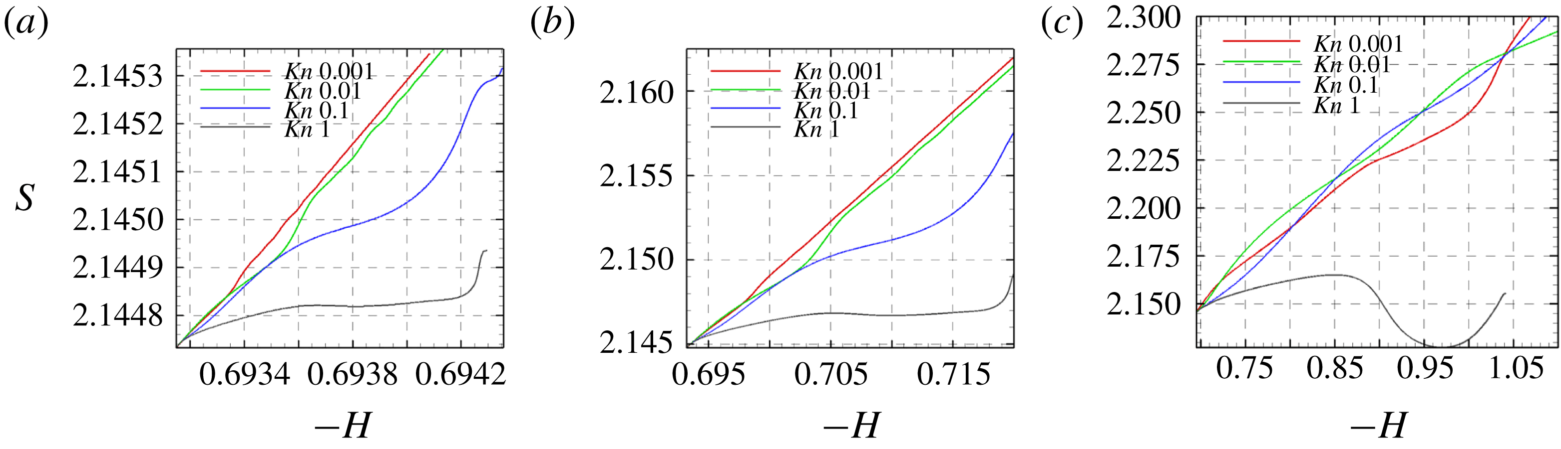
. It can be seen that
 $S_{tr}$
increases monotonically and maintains a direct proportionality with
 $-H$
for low Knudsen number (continuum and near-continuum) flows. This can be attributed to the absence of non-equilibrium effects within the system. With an increase in the degree of rarefaction,
 $S_{tr}$
does not grow linearly or even decreases as
 $-H$
increases.
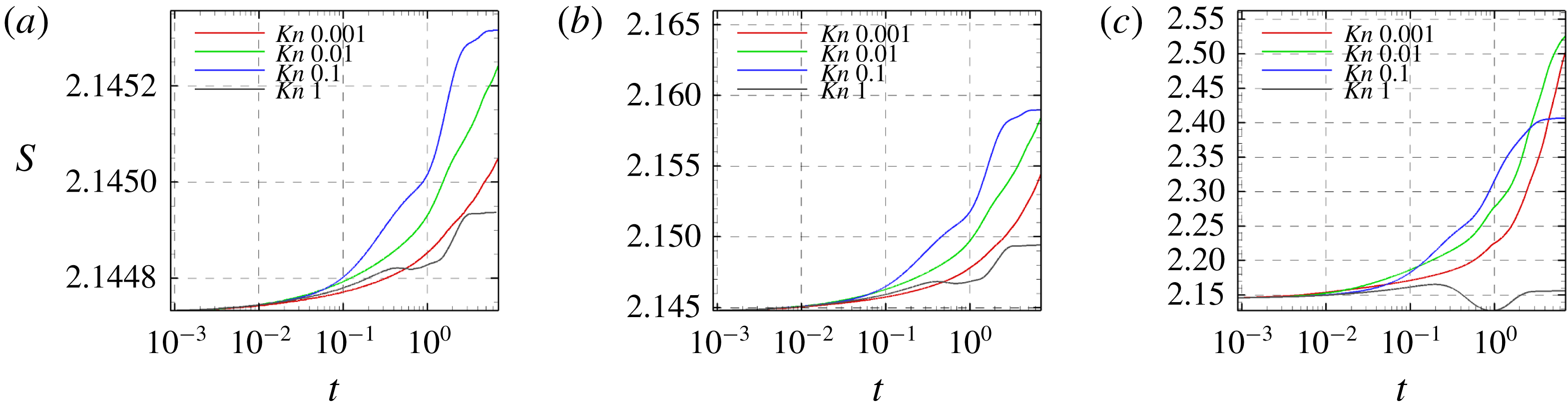
To further explain the above observations, we plot the temporal evolution of
 $S_{tr}$
and
 $-H$
for different cases in figures 17 and 18. As shown in figure 17,
 $S_{tr}$
experiences monotonic growth only for continuum or near-continuum cases. On the other hand,
 $-H$
increases monotonically at all Knudsen and Mach numbers. This implies that the time rate of change of
 $H$
is negative, upholding the entropy stipulation of
 $H$
-theorem. Therefore, it is clear that the Sackur–Tetrode entropy criterion is valid or near valid only in continuum flows where regions of high non-equilibrium transport are not dominant. Recall that the Sackur–Tetrode entropy presumes thermodynamic state variables at equilibrium. The contribution to entropy increase due to the non-equilibrium effects like the extreme rarefaction effects and velocity slip/temperature jump effects at the cavity walls must also be taken into account in order to obtain a correct estimate of the entropy in the system.
From the results, we conclude the following:
(a) In the continuum and near-continuum regimes, the UGKS numerical scheme is consistent with the Sackur–Tetrode entropy formulation.
(b) The UGKS thermal transport, even in the presence of significant co-gradient heat flux, is fully consistent with Boltzmann
$H$
–theorem at all degrees of rarefaction. This is not entirely surprising since the UGKS methodology is developed within the constraints of
$H$
–theorem.


Evolution of
 $S_{tr}$
with
 $-H$
(a)
 $M_{lid}=0.1$
, (b)
 $M_{lid}=0.5$
, (c)
 $M_{lid}=3.0$
.

Evolution of
 $S_{tr}$
with time (a)
 $M_{lid}=0.1$
(b)
 $M_{lid}=0.5$
(c)
 $M_{lid}=3.0$
.

Evolution of
 $-H$
with time (a)
 $M_{lid}=0.1$
, (b)
 $M_{lid}=0.5$
, (c)
 $M_{lid}=3.0$
.

6 Conclusion
The goal of this work is to characterize thermal transport over a range of Knudsen and Mach numbers. The UGKS numerical approach is used to simulate transport within driven cavities of various shapes. The UGKS temperature distribution and thermal flux alignment within the cavity are compared against the Fourier law and two extended thermodynamic models. The main findings of the study can be summarized as follows:
(a) The temperature distribution within the cavity is a strong function of the Knudsen and Mach numbers. At low Knudsen numbers, the cavity centre region experiences a high temperature due to the predominance of molecular collisions. With increasing Knudsen number (at fixed Mach number), the high temperature region shifts to the downstream wall. This is due to the fact that intermolecular collision frequency decreases, while collisions with the wall remain relatively unchanged.
(b) The ratio of the maximum-to-stagnation temperatures decreases with increasing Knudsen and Mach numbers.
(c) When the Mach number increases (at fixed Knudsen number), a recirculation region develops in the lower parts of the cavity. This is due to entrapment of molecules that collide more frequently than in the upper region. In this region, continuum-like conditions prevail even at high Knudsen numbers.
(d) The alignment of the thermal flux vector in cavities with very mild temperature gradients (low Knudsen and Mach numbers) is not well captured by the Fourier model even in the continuum limit. With only the first-order gradient term in the constitutive equation, the Fourier model is inherently incapable of capturing the nearly insignificant level of flux in these cases. In most cases, the error incurred by the Fourier model can be considered negligible as the flux magnitude is very small. Higher-order models capture the alignment of these low magnitude fluxes more precisely.
(e) In the continuum and near-continuum regimes, the Fourier model agrees well with UGKS fluxes at higher Mach numbers wherein the temperature gradients are reasonably large.
(f) In the transition and rarefied regimes, the Fourier model is deficient in the upper rarefied region of the cavity. It performs better in the lower recirculation region wherein continuum-like conditions prevail.
(g) Thermal fluxes computed from both the extended thermodynamic models are accurate throughout the domain in the continuum and near-continuum regimes. In the rarefied regime, both extended thermodynamic models are reasonably accurate in the interior of the cavity. The BGK-Burnett model is more accurate than the augmented Burnett model for low-speed flows. The opposite is seen for high-speed flows.
(h) Near the wall, regions of velocity slip and temperature jump appear with increasing Knudsen number. This in turn leads to non-equilibrium effects that permeate into the cavity interior. Even with the inclusion of higher-order terms, the augmented Burnett and BGK-Burnett models fail to predict these non-equilibrium effects near the wall adequately.
This study is the first in a series of investigations to characterize thermal and momentum transport in rarefied flows. The results of this study help to identify crucial aspects of thermal transport alignment in rarefied flows in different speed regimes. The strengths and weaknesses of popular extended thermodynamic models are also identified. In future studies, the thermal flux magnitudes will be examined. Further, momentum transport will also be investigated as a function of Mach and Knudsen numbers.
Appendix A. Flux expressions in extended thermodynamic models
The augmented Burnett heat flux components for a 2-D flow are given as:
 $$\begin{eqnarray}\displaystyle q_{x}^{(AB)} & = & \displaystyle q_{x}^{(0)}+q_{x}^{(1)}+\frac{\unicode[STIX]{x1D707}^{2}}{\unicode[STIX]{x1D70C}}\left(\unicode[STIX]{x1D6FE}_{1}\frac{1}{T}T_{x}u_{x}+\unicode[STIX]{x1D6FE}_{2}\frac{1}{T}T_{x}v_{y}+\unicode[STIX]{x1D6FE}_{3}u_{xx}+\unicode[STIX]{x1D6FE}_{4}u_{yy}+\unicode[STIX]{x1D6FE}_{5}v_{xy}+\unicode[STIX]{x1D6FE}_{6}\frac{1}{T}T_{y}v_{x}\right.\nonumber\\ \displaystyle & & \displaystyle +\left.\unicode[STIX]{x1D6FE}_{7}\frac{1}{T}T_{y}u_{y}+\unicode[STIX]{x1D6FE}_{8}\frac{1}{\unicode[STIX]{x1D70C}}\unicode[STIX]{x1D70C}_{x}u_{x}+\unicode[STIX]{x1D6FE}_{9}\frac{1}{\unicode[STIX]{x1D70C}}\unicode[STIX]{x1D70C}_{x}v_{y}+\unicode[STIX]{x1D6FE}_{10}\frac{1}{\unicode[STIX]{x1D70C}}\unicode[STIX]{x1D70C}_{y}u_{y}+\unicode[STIX]{x1D6FE}_{11}\frac{1}{\unicode[STIX]{x1D70C}}\unicode[STIX]{x1D70C}_{y}v_{x}\right)\nonumber\\ \displaystyle & & \displaystyle +\,\frac{\unicode[STIX]{x1D707}^{3}R}{p\unicode[STIX]{x1D70C}}\left(\unicode[STIX]{x1D6FE}_{12}T_{xxx}+\unicode[STIX]{x1D6FE}_{12}T_{xyy}+\unicode[STIX]{x1D6FE}_{13}\frac{T}{\unicode[STIX]{x1D70C}}\unicode[STIX]{x1D70C}_{xxx}+\unicode[STIX]{x1D6FE}_{13}\frac{T}{\unicode[STIX]{x1D70C}}\unicode[STIX]{x1D70C}_{xyy}\right),\end{eqnarray}$$
 $$\begin{eqnarray}\displaystyle q_{y}^{(AB)} & = & \displaystyle q_{y}^{(0)}+q_{y}^{(1)}+\frac{\unicode[STIX]{x1D707}^{2}}{\unicode[STIX]{x1D70C}}\left(\unicode[STIX]{x1D6FE}_{1}\frac{1}{T}T_{y}u_{y}+\unicode[STIX]{x1D6FE}_{2}\frac{1}{T}T_{y}v_{x}+\unicode[STIX]{x1D6FE}_{3}v_{yy}+\unicode[STIX]{x1D6FE}_{4}v_{xx}+\unicode[STIX]{x1D6FE}_{5}u_{xy}+\unicode[STIX]{x1D6FE}_{6}\frac{1}{T}T_{x}u_{y}\right.\nonumber\\ \displaystyle & & \displaystyle +\left.\unicode[STIX]{x1D6FE}_{7}\frac{1}{T}T_{x}v_{x}+\unicode[STIX]{x1D6FE}_{8}\frac{1}{\unicode[STIX]{x1D70C}}\unicode[STIX]{x1D70C}_{y}v_{y}+\unicode[STIX]{x1D6FE}_{9}\frac{1}{\unicode[STIX]{x1D70C}}\unicode[STIX]{x1D70C}_{y}u_{x}+\unicode[STIX]{x1D6FE}_{10}\frac{1}{\unicode[STIX]{x1D70C}}\unicode[STIX]{x1D70C}_{x}v_{x}+\unicode[STIX]{x1D6FE}_{11}\frac{1}{\unicode[STIX]{x1D70C}}\unicode[STIX]{x1D70C}_{x}u_{y}\right)\nonumber\\ \displaystyle & & \displaystyle +\,\frac{\unicode[STIX]{x1D707}^{3}R}{p\unicode[STIX]{x1D70C}}\left(\unicode[STIX]{x1D6FE}_{12}T_{yyy}+\unicode[STIX]{x1D6FE}_{12}T_{xxy}+\unicode[STIX]{x1D6FE}_{13}\frac{T}{\unicode[STIX]{x1D70C}}\unicode[STIX]{x1D70C}_{yyy}+\unicode[STIX]{x1D6FE}_{13}\frac{T}{\unicode[STIX]{x1D70C}}\unicode[STIX]{x1D70C}_{xxy}\right).\end{eqnarray}$$
The BGK-Burnett heat flux components are given by:
 $$\begin{eqnarray}\displaystyle q_{x}^{(BB)} & = & \displaystyle q_{x}^{(0)}+q_{x}^{(1)}+\frac{\unicode[STIX]{x1D707}^{2}}{\unicode[STIX]{x1D70C}}\left(\unicode[STIX]{x1D6FE}_{1}\frac{1}{T}T_{x}u_{x}+\unicode[STIX]{x1D6FE}_{2}\frac{1}{T}T_{x}v_{y}+\unicode[STIX]{x1D6FE}_{3}u_{xx}+\unicode[STIX]{x1D6FE}_{4}u_{yy}+\unicode[STIX]{x1D6FE}_{5}v_{xy}+\unicode[STIX]{x1D6FE}_{6}\frac{1}{T}T_{y}v_{x}\right.\nonumber\\ \displaystyle & & \displaystyle +\left.\unicode[STIX]{x1D6FE}_{7}\frac{1}{T}T_{y}u_{y}+\unicode[STIX]{x1D6FE}_{8}\frac{1}{\unicode[STIX]{x1D70C}}\unicode[STIX]{x1D70C}_{x}u_{x}+\unicode[STIX]{x1D6FE}_{9}\frac{1}{\unicode[STIX]{x1D70C}}\unicode[STIX]{x1D70C}_{x}v_{y}+\unicode[STIX]{x1D6FE}_{10}\frac{1}{\unicode[STIX]{x1D70C}}\unicode[STIX]{x1D70C}_{y}u_{y}+\unicode[STIX]{x1D6FE}_{11}\frac{1}{\unicode[STIX]{x1D70C}}\unicode[STIX]{x1D70C}_{y}v_{x}\right)\nonumber\\ \displaystyle & & \displaystyle +\,\frac{\unicode[STIX]{x1D707}^{3}}{p\unicode[STIX]{x1D70C}}\left(R\unicode[STIX]{x1D703}_{1}\left(T_{xxx}+T_{xyy}-\frac{1}{\unicode[STIX]{x1D70C}}\unicode[STIX]{x1D70C}_{x}T_{xx}-\frac{1}{\unicode[STIX]{x1D70C}}\unicode[STIX]{x1D70C}_{x}T_{yy}\right)+\unicode[STIX]{x1D703}_{2}u_{x}u_{xx}+\unicode[STIX]{x1D703}_{3}u_{x}v_{xy}+\unicode[STIX]{x1D703}_{4}u_{x}u_{yy}\right.\nonumber\\ \displaystyle & & \displaystyle +\,\unicode[STIX]{x1D703}_{5}v_{y}u_{xx}+\unicode[STIX]{x1D703}_{6}v_{y}v_{xy}+\unicode[STIX]{x1D703}_{7}v_{y}u_{yy}+\unicode[STIX]{x1D703}_{8}u_{y}v_{xx}+\unicode[STIX]{x1D703}_{9}u_{y}u_{xy}+\unicode[STIX]{x1D703}_{4}u_{y}v_{yy}+\unicode[STIX]{x1D703}_{8}v_{x}v_{xx}\nonumber\\ \displaystyle & & \displaystyle +\,\unicode[STIX]{x1D703}_{9}v_{x}u_{xy}+\unicode[STIX]{x1D703}_{4}v_{x}v_{yy}-\left(\frac{\unicode[STIX]{x1D70C}_{x}}{\unicode[STIX]{x1D70C}}+\frac{T_{x}}{T}\right) (\unicode[STIX]{x1D703}_{10}u_{x}^{2}+2\unicode[STIX]{x1D703}_{11}u_{x}v_{y}+2\unicode[STIX]{x1D703}_{12}u_{y}v_{x}+\unicode[STIX]{x1D703}_{12}u_{y}^{2}\nonumber\\ \displaystyle & & \displaystyle +\left.\unicode[STIX]{x1D703}_{12}v_{x}^{2}+\unicode[STIX]{x1D703}_{10}v_{y}^{2} )+\frac{R\unicode[STIX]{x1D703}_{1}}{T}(T_{x}T_{xx}+T_{x}T_{yy})\right),\end{eqnarray}$$
 $$\begin{eqnarray}\displaystyle q_{y}^{(BB)} & = & \displaystyle q_{y}^{(0)}+q_{y}^{(1)}+\frac{\unicode[STIX]{x1D707}^{2}}{\unicode[STIX]{x1D70C}}\left(\unicode[STIX]{x1D6FE}_{1}\frac{1}{T}T_{y}u_{y}+\unicode[STIX]{x1D6FE}_{2}\frac{1}{T}T_{y}v_{x}+\unicode[STIX]{x1D6FE}_{3}v_{yy}+\unicode[STIX]{x1D6FE}_{4}v_{xx}+\unicode[STIX]{x1D6FE}_{5}u_{xy}+\unicode[STIX]{x1D6FE}_{6}\frac{1}{T}T_{x}u_{y}\right.\nonumber\\ \displaystyle & & \displaystyle +\left.\unicode[STIX]{x1D6FE}_{7}\frac{1}{T}T_{x}v_{x}+\unicode[STIX]{x1D6FE}_{8}\frac{1}{\unicode[STIX]{x1D70C}}\unicode[STIX]{x1D70C}_{y}v_{y}+\unicode[STIX]{x1D6FE}_{9}\frac{1}{\unicode[STIX]{x1D70C}}\unicode[STIX]{x1D70C}_{y}u_{x}+\unicode[STIX]{x1D6FE}_{10}\frac{1}{\unicode[STIX]{x1D70C}}\unicode[STIX]{x1D70C}_{x}v_{x}+\unicode[STIX]{x1D6FE}_{11}\frac{1}{\unicode[STIX]{x1D70C}}\unicode[STIX]{x1D70C}_{x}u_{y}\right)\nonumber\\ \displaystyle & & \displaystyle +\,\frac{\unicode[STIX]{x1D707}^{3}}{p\unicode[STIX]{x1D70C}}\left(R\unicode[STIX]{x1D703}_{1}\left(T_{yyy}+T_{xxy}-\frac{1}{\unicode[STIX]{x1D70C}}\unicode[STIX]{x1D70C}_{y}T_{yy}-\frac{1}{\unicode[STIX]{x1D70C}}\unicode[STIX]{x1D70C}_{y}T_{xx}\right)+\unicode[STIX]{x1D703}_{2}v_{y}v_{yy}+\unicode[STIX]{x1D703}_{3}v_{y}u_{xy}+\unicode[STIX]{x1D703}_{4}v_{y}v_{xx}\right.\nonumber\\ \displaystyle & & \displaystyle +\,\unicode[STIX]{x1D703}_{5}u_{x}v_{yy}+\unicode[STIX]{x1D703}_{6}u_{x}u_{xy}+\unicode[STIX]{x1D703}_{7}u_{x}v_{xx}+\unicode[STIX]{x1D703}_{8}v_{x}u_{yy}+\unicode[STIX]{x1D703}_{9}v_{x}v_{xy}+\unicode[STIX]{x1D703}_{4}v_{x}u_{xx}+\unicode[STIX]{x1D703}_{8}u_{y}u_{yy}\nonumber\\ \displaystyle & & \displaystyle +\,\unicode[STIX]{x1D703}_{9}u_{y}v_{xy}+\unicode[STIX]{x1D703}_{4}u_{y}u_{xx}-\left(\frac{\unicode[STIX]{x1D70C}_{y}}{\unicode[STIX]{x1D70C}}+\frac{T_{y}}{T}\right) (\unicode[STIX]{x1D703}_{10}u_{x}^{2}+2\unicode[STIX]{x1D703}_{11}u_{x}v_{y}+2\unicode[STIX]{x1D703}_{12}u_{y}v_{x}+\unicode[STIX]{x1D703}_{12}u_{y}^{2}\nonumber\\ \displaystyle & & \displaystyle +\left.\unicode[STIX]{x1D703}_{12}v_{x}^{2}+\unicode[STIX]{x1D703}_{10}v_{y}^{2} )+\frac{R\unicode[STIX]{x1D703}_{1}}{T}(T_{y}T_{xx}+T_{y}T_{yy})\right).\end{eqnarray}$$
The coefficients for argon gas (Agarwal & Balakrishnan Reference Agarwal and Balakrishnan1996) from
 $\unicode[STIX]{x1D6FE}_{1}$
through
 $\unicode[STIX]{x1D6FE}_{14}$
are
 $-11.101$
,
 $-1.0$
,
 $-1.384$
,
 $-2.0$
,
 $-3.333$
,
 $-6.5$
,
 $-5.667$
,
 $-1.051$
,
 $1.0$
,
 $-3.0$
,
 $-3.0$
,
 $0.6875$
and
 $-0.625$
respectively; and from
 $\unicode[STIX]{x1D703}_{1}$
through
 $\unicode[STIX]{x1D703}_{12}$
are
 $4.167$
,
 $6.222$
,
 $-1.778$
,
 $1.333$
,
 $-3.111$
,
 $4.222$
,
 $-0.667$
,
 $4.333$
,
 $3.667$
,
 $2.222$
,
 $-1.111$
and
 $1.667$
respectively.