1 Introduction
Consider the Kolmogorov system

where
$x_i$
 is the population density of the ith species, and
$f_i$
 is the per capita growth rate of the ith species in the variables
$x=(x_{1},\ x_{2},\ \ldots ,\ x_{n})\in \mathbb {R}^{n}_{+}$
 . Hereafter,
$\mathbb R_+$
 is the set of nonnegative real numbers. In the case that
$f=(f_{1},\ f_{2},\ \ldots ,\ f_{n}): \mathbb {R}^{n}_{+}\rightarrow \mathbb {R}^{n}$
 is a
${C}^{1}$
 map, such a system is called a type- K monotone system if the Jacobian matrix
$\mathrm {D}f(x)$
 of f has the form

where
$A_{1}$
 is an
$m\times m$
 matrix,
$A_{2}$
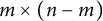
 is an
$m\times (n-m)$
 matrix,
$A_{3}$
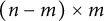
 is an
$(n-m)\times m$
 matrix,
$A_{4}$
 is an
$(n-m)\times (n-m)$
 matrix with
$0\leq m\leq n-1$
 , and each off-diagonal element of
$A_{1}$
 and
$A_{4}$
 is nonnegative, and
$A_{2}$
 and
$A_{3}$
 are nonnegative matrices. Under this setting, the species could be divided into two subgroups
$I:=\{x_i|\ i\in \{1,2,\ldots ,m\}\}$
 and
$J:=\{x_j|\ j\in \{m+1,m+2,\ldots ,n\}\}$
 , in such a way that the species in subgroup I form a mutualistic or cooperative subcommunity, while the species in subgroup J form a cooperative subcommunity. And the species in the subgroup I compete with the species in the subgroup J. System (1.1) is a generalization of the extended Lotka–Volterra system

where
$x_i$
 is again the population density of the ith species,
$r=(r_1,\ r_2, \ldots , r_n)^{\tau }$
 is the vector of intrinsic growth rates, and
$a_{ij}$
 represents the effect of interspecific (if
$i\neq j$
 ) or intraspecific (if
$i=j$
 ) interaction.
On study of dynamics of the systems of form (1.2) which are in the type-K monotone, there is a long history. Takeuchi, Adachi, and Tokumaru [Reference Takeuchi, Adachi and Tokumaru14] in 1978, Travis and Post [Reference Travis and Post15] in 1979, and Takeuchi and Adachi [Reference Takeuchi and Adachi13] in 1980 studied its long term behaviors without explicitly using the monotonicity properties of the systems. Precisely, by applying the results from mathematical programming and Lyapunov function arguments (due to Goh [Reference Goh2]) to the type-K monotone Lotka–Volterra system (1.2), Takeuchi and Adachi [Reference Takeuchi and Adachi13] in 1980 got a remarkable result, which can be stated as: if the coefficient matrix
$A=(a_{ij})$
 of (1.2) is stable, then the system possesses an equilibrium attracting all positive initial points. Smith [Reference Smith11] in 1986 extended Hirsch’s ideas for the cooperative systems to the type-K monotone systems of form (1.1) and obtained sufficient conditions for persistence of all species. Smith [Reference Smith11] in 1986 and [Reference Smith12] in 1988 proved by the theory of monotone semiflow that the type-K monotone system (1.2) admits a globally asymptotically stable equilibrium in the interior of the positive octant if the intrinsic growth rates are all positive, the coefficient matrix A is stable and either of the two cooperative subcommunities of system (1.2) admits a globally asymptotically stable equilibrium in the interior of the space which is unstable to its complementary space. Tu and Jiang [Reference Tu and Jiang16] in 1998, [Reference Tu and Jiang17, Reference Tu and Jiang18] in 1999 and Liang and Jiang [Reference Liang and Jiang8] in 2002 provided the necessary and sufficient conditions for the type-K monotone system (1.2) to have a globally asymptotically stable positive equilibrium. Liang and Jiang [Reference Liang and Jiang7] in 2002 classified the finite dynamics of the type-K monotone Lotka–Volterra system (1.2) for
$n=3$
 , and obtained 16 different classes of phase portraits without assuming the identical intrinsic growth rates but with all equilibria being hyperbolic. Here, the finite dynamics means the dynamics that do not include the ones at infinity. We mention that Zeeman [Reference Zeeman19] defined a combinatorial equivalence relation among three dimensional competitive Lotka–Volterra systems by its nullclines and classified them into
$33$
 stable nullcline classes, with
$27$
 of which admitting no periodic orbits, so their finite dynamics can be fully described. Llibre and Martinez [Reference Llibre and Martínez10] classified a three-dimensional competitive Lotka–Volterra system with different intrinsic growth rates and the same interspecific and intraspecific interactions in the positive octant of the Poincaré ball, whose carrying simplex is a flat triangle and finite dynamics belongs to Zeeman’s class
$1$
 . The remaining 6 cases in the Zeeman’s 33 classes may posses limit cycles. But how many limit cycles they have still remains open (see [Reference Li and Jiang5] and references therein). The similar work was done by Liang and Jiang [Reference Liang and Jiang9] for three dimensional type-K competitive Lotka–Volterra systems, especially they may admit limit cycles, but one cannot decide their number. There are no periodic orbits in 3D type-K monotone Lotka–Volterra systems, so their finite dynamics are simpler than those of 3D type-K competitive Lotka–Volterra systems.
In this paper, we will study global dynamics of the 3D type-K monotone Lotka–Volterra system with the identical intrinsic growth rate in
$\mathbb {R}^{3}_{+}$
 , i.e.,

where
$\mathbb R_+^3=\{(x_1,x_2,x_3)\in \mathbb R^3:\ x_1,x_2,x_3\ge 0\}$
 . By means of the replicator equations, we classify all global dynamics of system (1.3) in the first octant of the Poincaré ball under the assumption:
-
(H) Each equilibrium of the compactified vector field associated with system (1.3) in $\mathbb {R}^{3}_{+}$
 at infinity is hyperbolic.

Poincaré compatification was developed initially for studying dynamics of planar polynomial differential systems at infinity. This method was extended to any finite dimensional polynomial differential systems. For detailed information on Poincaré compactification applying to higher dimensional polynomial differential systems, see e.g., Cima and Llibre [Reference Cima and Llibre1]. Roughly speaking, Poincaré compactification in
$\mathbb R^3$
 defines in an equivalent way a vector field near the surface of the Poincaré ball (the compact unit ball centered at the origin), which is called Poincaré compactified vector field. It, after time rescaling, is still a polynomial one in each of the local charts.
With the help of Poincaré compactification in
$\mathbb R^3$
 , we classify here all global dynamics of system (1.3) in the first octant of
$\mathbb {R}^{3}$
 , i.e.,
$\{(x_1,x_2,x_3)\in \mathbb R^3:\ x_{1}\geq 0,\ x_{2}\geq 0,\ x_{3}\geq 0\}$
 under the assumption (H).
Define

and set

These quantities are traces and determinants of various (principal) minors of the matrix A. As we shall see in Section 3.1 system (1.3) has at most eight finite equilibria, which are the origin O, the finite equilibria

on the axes, the finite equilibria

in the interior of the coordinate planes and the positive finite equilibrium

Besides, system (1.3) has at most seven equilibria at the infinity of
$\mathbb {R}^{3}_{+}$
 , namely

Obviously, it follows from the signs of
$a_{ij}$
 that
$\alpha _{1}>0$
 and
$\beta _{2}>0$
 . The assumption (H) means that
$\alpha _{2}, \alpha _{3}, \beta _{1}, \beta _{3}, J_i\neq 0, \ i=1,\ 2,\ 3$
 . The local behaviors of the finite equilibria and the equilibria at infinity of system (1.3) are determined by the parameters
$\alpha _{2}, \alpha _{3}, \beta _{1}, \beta _{3}, I_{12}, J_{1}, J_{2}$
 , and
$J_{3}$
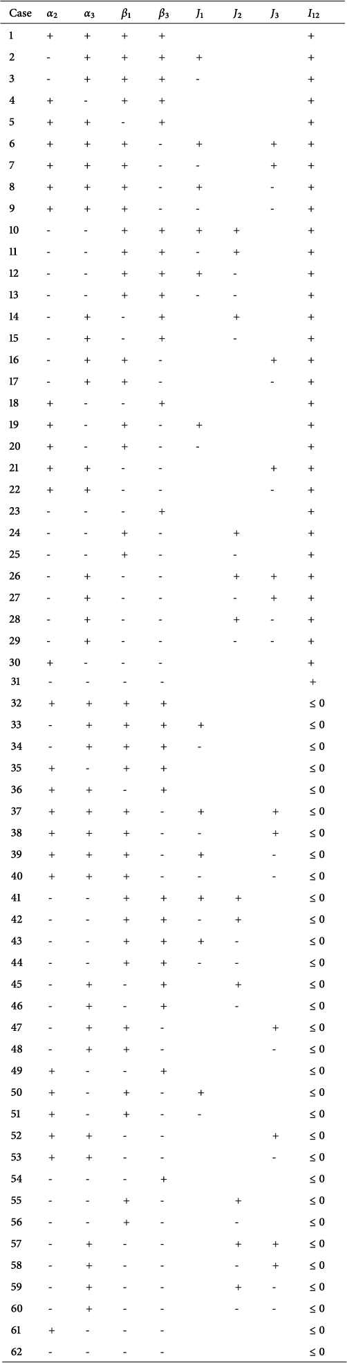
 . If system (1.3) satisfies the assumption (H), there are totally
$62$
 cases according to all the logical possibilities of the signs of these parameter values, which are listed in the following Table 4. We will determine which of these cases can be actually realized.
Having these local properties, we then study the topological classification of the corresponding replicator equations for the authentic systems in Section 5. By utilizing the configuration of the separatrices of the replicator equations, the invariant interfaces of system (1.3) in the Poincaré ball will be further constructed. These invariant interfaces together with the unstable manifolds of the saddles separate the Poincaré ball into mutually disjoint invariant domains, in each of which all trajectories have the same
$\alpha $
 -limit and
$\beta $
 -limit. Finally, combining these facts together with the expressions in (1.4), we characterize in Section 6 all global topological phase portraits of system (1.3), which are totally
$35$
 topologically different ones. As a by product of these classifications, we obtain the necessary and sufficient condition for all positive trajectories of system (1.3) in
$\mathbb {R}^{3}_{+}$
 to be bounded, that is, the
$2\times 2$
 principal minor
$I_{12}$
 of the coefficient matrix A is positive. We comment that the restriction of the identical intrinsic growth rate is essential in our study. Otherwise, the problem would become much involved, and, of course, there will be more topologically different phase portraits than 35. We hope that we will handle with this case in the future.
2 Statements of main results
As we mentioned previously, this paper focuses on the dynamics of system (1.3) in the first octant of
$\mathbb R^3$
 via the Poincaré compactification. To compactify system (1.3) in the Poincaré ball, we adopt the strategy in [Reference Cima and Llibre1]. Let
$\mathbb {S}^{3}$
 denote the unit sphere in
$\mathbb {R}^{4}$
 , and
$\mathbb {S}^{3}_{+}$
 the northern hemisphere. The tangent space to
$\mathbb {S}^{3}$
 at the point
$y\in \mathbb {S}^{3}$
 is denoted by
$T_{y}\mathbb {S}^{3}$
 . Then the tangent hyperplane
$T_{(0,\ 0,\ 0,\ 1)}\mathbb {S}^{3}$
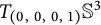 is identified with
$\mathbb {R}^{3}$
 . Let us consider the central projection
$f_{+}:\mathbb {R}^{3}=T_{(0,\ 0,\ 0,\ 1)}\mathbb {S}^{3}\rightarrow \mathbb {S}^{3}_{+}$
 defined by

where
$\Delta x=(1+x_{1}^{2}+x_{2}^{2}+x_{3}^{2})^{1/2}$
 . Through this central projection,
$\mathbb {R}^{3}$
 can be identified with
$\mathbb {S}^{3}_{+}\backslash \{y_{4}=0\}$
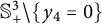 . By this central projection, the study of the properties of system (1.3) at infinity is turned to the corresponding system along the equator
$\mathbb {S}^{2}:=\left \{y\in \mathbb {S}^{3}: y_{4}=0\right \}$
 of the sphere
$\mathbb S^3$
 . To do so, taking the sphere coordinate transformation in
$\mathbb R^3$


with
$r\ge 1$
 . The points on the equator
$\mathbb {S}^{2}$
 are
$(\sin \theta \cos \varphi ,\ \sin \theta \sin \varphi , \ \cos \theta ,\ 0)$
 with
$\theta \in [0,\pi ]$
 and
$\varphi \in [0,2\pi ]$
 . Under this correspondence, if
$K_{1}$
 is a subset of
$\mathbb {R}^{3}$
 , then the subset inside the Poincaré ball which is identified with
$K_{1}$
 is denoted by
$p(K_{1})$
 . Thus for instance
$p((k_{1},\ k_{2},\ k_{3}))$
 denotes the point
$\left (\frac {k_{1}}{\Delta k},\ \frac {k_{2}}{\Delta k},\ \frac {k_{3}}{\Delta k}\right )$
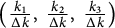 . Let us denote by
$\mathbb {D}$
 the set of the endpoints of the directional vectors
$(\sin \theta \cos \varphi , \ \sin \theta \sin \varphi , \ \cos \theta )$
 for
$\theta \in [0,\pi ]$
 and
$\varphi \in [0,2\pi ]$
 , i.e., the infinity of
$\mathbb {R}^{3}$
 . If
$K_{2}$
 is a subset of
$\mathbb {D}$
 , then the subset of the Poincaré sphere which is identified with
$K_{2}$
 through
$f_+$
 is also denoted by
$p(K_{2})$
 . Thus for instance if W is the positive endpoint of the line
$\{x_{2}=l_{1}x_{1}\}\cap \{x_{3}=l_{2}x_{1}\} (l_{1}>0, l_{2}>0)$
 then
$p(W)$
 denotes the point
$\left (\frac {1}{\sqrt {1+l_{1}^{2}+l_{2}^{2}}},\ \frac {l_{1}}{\sqrt {1+l_{1}^{2}+l_{2}^{2}}},\ \frac {l_{2}}{\sqrt {1+l_{1}^{2}+l_{2}^{2}}}\right )$
 . For more details on the Poincaré compactification in
$\mathbb {R}^{3}$
 , see e.g., [Reference Cima and Llibre1]. As usual we denote by
$\partial R$
 the boundary of

and by
$\mathrm {Int}R$
 the interior of R. Denote by
$\Sigma _+^\infty $
 the infinity of
$\mathbb R^3$
 in the positive octant, which according to the above correspondence can be treated as
$\partial R\cap \left \{x_{1}^{2}+x_{2}^{2}+x_{3}^{2}=1\right \}$
 . Next we shall state the flow of the compactified vector field associated with system (1.3) in the region R of
$\mathbb R^3$
 .
Theorem 2.1 (Global classification theorem)
Under the assumption (H), system (1.3) restricted to the positive octant has exactly
$35$
 topologically different global dynamics in the Poincaré compactification, which are listed in Table 5 together with the corresponding parameter conditions.
The next Theorems 2.2–2.8 present the concrete information on the dynamics in each of the 35 classes stated in Theorem 2.1.
Theorem 2.2 For the classes
$1$
 –
$5$
 in Table 5, the following statements hold.
-
(a) For the class $1$
, the phase portrait is topologically equivalent to Figure
$(1b)$
in Table 5, which contains two invariant domains limited by the invariant surface passing
$p(U_{12})$
and
$p(B_{i})$
for
$i=1, 2, 3$
. In the interior of one
$(resp.\ the\ other)$
of the domains all orbits have their
$\alpha $
-limits at
$O (resp. p(A_{1}))$
, and have their
$\omega $
-limits at
$p(U_{12})$
, which is the global attractor in
$\mathrm {Int}R$
. -
(b) For the class $2$
, the phase portrait is topologically equivalent to Figure
$(2b)$
in Table 5, which contains four invariant domains limited by the invariant surface passing
$ p(U_{12}),\ p(U_{23})$
, and
$p(B_{i})$
for
$i=1, 2, 3$
and the invariant surface passing
$O,\ p(B_{1}),\ p(A_{1}),\ p(U_{23})$
, and
$p(V_{23})$
. In the interior of the two domains nearby O all orbits have their
$\alpha $
-limits at O, and their
$\omega $
-limits at either
$p(U_{12})$
or
$p(B_{3})$
. In the interior of the other two domains all orbits have their
$\alpha $
-limits at
$p(A_{1})$
, and their
$\omega $
-limits at either
$p(U_{12})$
or
$p(B_{3})$
. -
(c) For the class $3$
, the phase portrait is topologically equivalent to Figure
$(3b)$
in Table 5, which contains six invariant domains limited by the invariant surface passing
$p(U_{12})$
,
$ p(U_{23})$
,
$p(P)$
and
$p(B_{i})$
for
$i=1, 2, 3$
, the invariant surface passing O,
$p(B_{1})$
,
$p(A_{1})$
,
$p(P)$
,
$ p(Q)$
,
$ p(U_{23})$
and
$p(V_{23})$
, and the invariant surface passing
$p(B_{3})$
,
$ p(A_{3})$
,
$ p(P)$
,
$ p(Q)$
,
$p(U_{12})$
and
$p(V_{12})$
. In the interior of the two domains adjoin O all orbits have their
$\alpha $
-limits at O, and their
$\omega $
-limits at either
$p(U_{12})$
or
$p(B_{3})$
. In the interior of the two domains adjoin the line segment between
$p(A_3)$
and
$p(B_3)$
all orbits have their
$\alpha $
-limits at either
$p(A_{1})$
or
$p(V_{23})$
, and their
$\omega $
-limits at
$p(B_{3})$
. In the interior of the two domains adjoin the line segment between
$p(U_{12})$
and
$p(V_{12})$
all orbits have their
$\alpha $
-limits at either
$p(A_{1})$
or
$p(V_{23})$
, and their
$\omega $
-limits at
$p(U_{12})$
. -
(d) For the class $4$
, the phase portrait is topologically equivalent to Figure
$(4b)$
in Table 5, which contains two invariant domains limited by the invariant surface passing
$p(U_{12}),\ p(U_{13})$
, and
$p(B_{i})$
for
$i=1, 2, 3$
. In the interior of the two domains all orbits have their
$\alpha $
-limits at either O or
$p(V_{13})$
, and their
$\omega $
-limits at
$p(U_{12})$
, which is the global attractor in
$\mathrm {Int}R$
. -
(e) For the class $5$
, the phase portrait is topologically equivalent to Figure
$(5b)$
in Table 5, which contains three invariant domains limited by the invariant surface passing
$p(U_{12}),\ p(U_{13})$
, and
$p(B_{i})$
for
$i=1, 2, 3$
and the invariant surface passing
$p(U_{12}),\ p(U_{13}),\ p(V_{12})$
, and
$p(V_{13})$
. In the interior of the domain adjoin O all orbits have their
$\alpha $
-limit at O, and their
$\omega $
-limit at
$p(U_{12})$
. In the interior of the other two domains all orbits have their
$\alpha $
-limits at either
$p(A_{1})$
or
$p(A_{3})$
, and their
$\omega $
-limits at
$p(U_{12})$
, which is the global attractor in
$\mathrm {Int}R$
.






















Theorem 2.3 For the classes
$6$
 –
$10$
 in Table 5, the following statements hold.
-
(a) For the class $6$
, the phase portrait is topologically equivalent to Figure
$(6b)$
in Table 5, which contains three invariant domains limited by the invariant surface passing
$p(U_{12})$
,
$p(U_{23})$
,
$ p(P)$
, and
$p(B_{i})$
for
$i=1, 2, 3$
and the invariant surface passing
$p(U_{12})$
,
$ p(V_{12})$
,
$p(P)$
,
$p(Q)$
,
$p(U_{23})$
, and
$p(V_{23})$
. In the interior of the domain adjoin O all orbits have their
$\alpha $
-limits at O, and their
$\omega $
-limits at
$p(P)$
. In the interior of the other two domains all orbits have their
$\alpha $
-limits at either
$p(A_{1})$
or
$p(A_{2})$
, and their
$\omega $
-limits at
$p(P)$
, which is the global attractor in
$\mathrm {Int}R$
. -
(b) For the class $7$
, the phase portrait is topologically equivalent to Figure
$(7b)$
in Table 5, which contains three invariant domains limited by the invariant surface passing
$p(U_{12}),\ p(U_{23})$
, and
$p(B_{i})$
for
$i=1, 2, 3$
and the invariant surface passing
$p(U_{12}),\ p(V_{12}),\ p(U_{23})$
, and
$p(V_{23})$
. In the interior of the domain adjoin O all orbits have their
$\alpha $
-limits at O, and their
$\omega $
-limits at
$p(U_{12})$
. In the interior of the other two domains all orbits have their
$\alpha $
-limits at either
$p(A_{1})$
or
$p(A_{2})$
, and their
$\omega $
-limits at
$p(U_{12})$
, which is the global attractor in
$\mathrm {Int}R$
. -
(c) For the class $8$
, the phase portrait is topologically equivalent to Figure
$(8b)$
in Table 5, which contains six invariant domains limited by the invariant surface passing
$p(U_{12})$
,
$p(U_{23})$
,
$p(P)$
, and
$p(B_{i})$
for
$i=1, 2, 3$
, the invariant surface passing O,
$p(B_{1})$
,
$ p(A_{1})$
,
$p(P)$
,
$p(Q)$
,
$ p(B_{2})$
, and
$p(A_{2})$
, and the invariant surface passing
$p(U_{12})$
,
$p(V_{12})$
,
$p(P)$
,
$p(Q)$
,
$p(U_{23})$
, and
$p(V_{23})$
. In the interior of the two domains adjoin O all orbits have their
$\alpha $
-limits at O, and their
$\omega $
-limits at either
$p(U_{12})$
or
$p(U_{23})$
. In the interior of the two domains adjoin the line segment between
$p(U_{12})$
and
$p(V_{12})$
all orbits have their
$\alpha $
-limits at either
$p(A_{1})$
or
$p(A_{2})$
, and their
$\omega $
-limits at
$p(U_{12})$
. In the interior of the two domains adjoin the line segment between
$p(U_{23})$
and
$p(V_{23})$
all orbits have their
$\alpha $
-limits at either
$p(A_{1})$
or
$p(A_{2})$
, and their
$\omega $
-limits at
$p(U_{23})$
. -
(d) For the class $9$
, the phase portrait is topologically equivalent to Figure
$(9b)$
in Table 5, which contains four invariant domains limited by the invariant surface passing
$ p(U_{12})$
,
$p(U_{13})$
,
$ p(U_{23})$
, and
$p(B_{i})$
for
$i=1, 2, 3$
and the invariant surface passing O,
$p(U_{13})$
,
$p(V_{13})$
,
$ p(U_{23})$
, and
$p(V_{23})$
. In the interior of the two domains adjoin O all orbits have their
$\alpha $
-limits at O, and their
$\omega $
-limits at either
$p(U_{12})$
or
$p(B_{3})$
. In the interior of the other two domains all orbits have their
$\alpha $
-limits at
$p(V_{23})$
, and their
$\omega $
-limits at either
$p(U_{12})$
or
$p(B_{3})$
. -
(e) For the class $10$
, the phase portrait is topologically equivalent to Figure
$(10b)$
in Table 5, which contains six invariant domains limited by the invariant surface passing
$p(U_{12})$
,
$p(U_{13})$
,
$p(U_{23})$
,
$ p(P)$
, and
$p(B_{i})$
for
$i=1, 2, 3$
, the invariant surface passing O,
$p(U_{13})$
,
$p(V_{13})$
,
$p(P)$
,
$p(Q)$
,
$p(U_{23})$
, and
$p(V_{23})$
, and the invariant surface passing
$p(B_{3}),\ p(A_{3}),\ p(P),\ p(Q),\ p(U_{12})$
, and
$p(V_{12})$
. In the interior of the two domains adjoin O all orbits have their
$\alpha $
-limits at O, and their
$\omega $
-limits at either
$p(U_{12})$
or
$p(B_{3})$
. In the interior of the two domains adjoin the line segment between
$p(A_3)$
and
$p(B_3)$
all orbits have their
$\alpha $
-limits at either
$p(V_{13})$
or
$p(V_{23})$
, and their
$\omega $
-limits at
$p(B_{3})$
. In the interior of the two domains adjoin the line segment between
$p(U_{12})$
and
$p(V_{12})$
all orbits have their
$\alpha $
-limits at either
$p(V_{13})$
or
$p(V_{23})$
, and their
$\omega $
-limits at
$p(U_{12})$
.











Theorem 2.4 For the classes
$11$
 –
$15$
 in Table 5, the following statements hold.
-
(a) For the class $11$
, the phase portrait is topologically equivalent to Figure
$(11b)$
in Table 5, which contains three invariant domains limited by the invariant surface passing
$p(U_{12})$
,
$p(U_{13})$
,
$ p(U_{23})$
, and
$p(B_{i})$
for
$i=1, 2, 3$
and the invariant surface passing
$p(U_{12})$
,
$p(U_{13})$
,
$p(V_{12})$
, and
$p(V_{13})$
. In the interior of the domain adjoin O all orbits have their
$\alpha $
-limits at O, and their
$\omega $
-limits at
$p(U_{12})$
. In the interior of the other two domains all orbits have their
$\alpha $
-limits at either
$p(A_{1})$
or
$p(V_{23})$
, and their
$\omega $
-limits at
$p(U_{12})$
, which is the global attractor in
$\mathrm {Int}R$
. -
(b) For the class $12$
, the phase portrait is topologically equivalent to Figure
$(12b)$
in Table 5, which contains six invariant domains limited by the invariant surface passing
$p(U_{12})$
,
$ p(U_{13})$
,
$p(U_{23})$
,
$p(P)$
, and
$p(B_{i})$
for
$i=1, 2, 3$
, the invariant surface passing O,
$p(B_{1})$
,
$p(A_{1})$
,
$p(P)$
,
$p(Q)$
,
$p(U_{23})$
, and
$p(V_{23})$
, and the invariant surface passing
$p(U_{12})$
,
$p(V_{12})$
,
$p(P)$
,
$p(Q)$
,
$p(U_{13})$
, and
$p(V_{13})$
. In the interior of the two domains adjoin O all orbits have their
$\alpha $
-limits at O, and their
$\omega $
-limits at either
$p(U_{12})$
or
$p(U_{13})$
. In the interior of the two domains adjoin the line segment between
$p(U_{13})$
and
$p(V_{13})$
all orbits have their
$\alpha $
-limits at either
$p(A_{1})$
or
$p(V_{23})$
, and their
$\omega $
-limits at
$p(U_{13})$
. In the interior of the two domains adjoin the line segment between
$p(U_{12})$
and
$p(V_{12})$
all orbits have their
$\alpha $
-limits at either
$p(A_{1})$
or
$p(V_{23})$
, and their
$\omega $
-limits at
$p(U_{12})$
. -
(c) For the class $13$
, the phase portrait is topologically equivalent to Figure
$(13b)$
in Table 5, which contains three invariant domains limited by the invariant surface passing
$ p(U_{12})$
and
$p(B_{i})$
for
$i=1, 2, 3$
and the invariant surface passing
$p(B_{3}),\ p(A_{3}),\ p(U_{12})$
, and
$p(V_{12})$
. In the interior of the domain adjoin O all orbits have their
$\alpha $
-limits at O, and their
$\omega $
-limits at
$p(B_{3})$
. In the interior of the two domains all orbits have their
$\alpha $
-limits at either
$p(A_{1})$
or
$p(A_{2})$
, and their
$\omega $
-limits at
$p(B_{3})$
, which is the global attractor in
$\mathrm { Int}R$
. -
(d) For the class $14$
, the phase portrait is topologically equivalent to Figure
$(14b)$
in Table 5, which contains six invariant domains limited by the invariant surface passing
$p(U_{12}),\ p(P)$
, and
$p(B_{i})$
for
$i=1, 2, 3$
, the invariant surface passing O,
$p(B_{1})$
,
$p(A_{1})$
,
$p(P)$
,
$p(Q)$
,
$p(B_{2})$
, and
$p(A_{2})$
, and the invariant surface passing
$p(U_{12})$
,
$p(V_{12})$
,
$ p(P)$
,
$p(Q)$
,
$p(B_{3})$
, and
$p(A_{3})$
. In the interior of the two domains adjoin O all orbits have their
$\alpha $
-limits at O, and their
$\omega $
-limits at either
$p(U_{12})$
or
$p(B_{3})$
. In the interior of the two domains adjoin the line segment between
$p(B_3)$
and
$p(A_3)$
all orbits have their
$\alpha $
-limits at either
$p(A_{1})$
or
$p(A_{2})$
, and their
$\omega $
-limits at
$p(B_{3})$
. In the interior of the two domains adjoin the line segment between
$p(U_{12})$
and
$p(V_{12})$
all orbits have their
$\alpha $
-limits at either
$p(A_{1})$
or
$p(A_{2})$
, and their
$\omega $
-limits at
$p(U_{12})$
. -
(e) For the class $15$
, the phase portrait is topologically equivalent to Figure
$(15b)$
in Table 5, which contains two invariant domains limited by the invariant surface passing
$p(U_{12})$
and
$p(B_{i})$
for
$i=1, 2, 3$
. In the interior of the two domains all orbits have their
$\alpha $
-limits at either O or
$p(A_{3})$
, and their
$\omega $
-limits at
$p(U_{12})$
, which is the global attractor in
$\mathrm {Int}R$
.








Theorem 2.5 For the classes
$16$
 –
$20$
 in Table 5, the following statements hold.
-
(a) For the class $16$
, the phase portrait is topologically equivalent to Figure
$(16b)$
in Table 5, which contains four invariant domains limited by the invariant surface passing
$p(U_{12})$
,
$ p(U_{13})$
,
$p(U_{23})$
,
$p(P)$
, and
$p(B_{i})$
for
$i=1, 2, 3$
, the invariant surface passing
$p(U_{12})$
,
$p(V_{12})$
,
$p(P)$
, and
$p(Q)$
, the invariant surface passing
$p(U_{13})$
,
$p(V_{13})$
,
$p(P)$
, and
$p(Q)$
, and the invariant surface passing
$p(U_{23})$
,
$p(V_{23})$
,
$p(P)$
, and
$p(Q)$
. In the interior of the domain adjoin O all orbits have their
$\alpha $
-limits at O, and their
$\omega $
-limits at
$p(P)$
. In the interior of the domain adjoin the line segment between
$p(A_3)$
and
$p(B_3)$
all orbits have their
$\alpha $
-limits at
$p(A_{3})$
, and their
$\omega $
-limits at
$p(P)$
. In the interior of the other two domains all orbits have their
$\alpha $
-limits at either
$p(A_{1})$
or
$p(A_{2})$
, and their
$\omega $
-limits at
$p(P)$
, which is the global attractor in
$\mathrm {Int}R$
. -
(b) For the class $17$
, the phase portrait is topologically equivalent to Figure
$(17b)$
in Table 5, which contains four invariant domains limited by the invariant surface passing
$p(U_{12})$
,
$p(U_{13})$
,
$p(U_{23})$
, and
$p(B_{i})$
for
$i=1, 2, 3$
, the invariant surface passing
$p(U_{12})$
,
$p(V_{12})$
,
$p(U_{13})$
, and
$p(V_{13})$
, and the invariant surface passing
$p(U_{12})$
,
$p(V_{12})$
,
$p(U_{23})$
, and
$p(V_{23})$
. In the interior of the domain adjoin O all orbits have their
$\alpha $
-limits at O, and their
$\omega $
-limits at
$p(U_{12})$
. In the interior of the other three domains all orbits have their
$\alpha $
-limits at either
$p(A_{1})$
or
$p(A_{2})$
or
$p(A_{3})$
, and their
$\omega $
-limits at
$p(U_{12})$
, which is the global attractor in
$\mathrm {Int}R$
. -
(c) For the class $18$
, the phase portrait is topologically equivalent to Figure
$(18b)$
in Table 5, which contains two invariant domains limited by the invariant surface passing
$p(V_{12})$
and
$p(B_{i})$
for
$i=1, 2, 3$
. In the interior of the two domains all orbits have their
$\alpha $
-limits at either O or
$p(A_{1})$
, and their
$\omega $
-limits at
$p(V_{12})$
, which is the global attractor in
$\mathrm {Int}R$
. -
(d) For the class $19$
, the phase portrait is topologically equivalent to Figure
$(19b)$
in Table 5, which contains four invariant domains limited by the invariant surface passing
$ p(V_{12})$
,
$p(U_{23})$
, and
$p(B_{i})$
for
$i=1, 2, 3$
and the invariant surface passing O,
$p(B_{1})$
,
$p(A_{1})$
,
$p(U_{23})$
, and
$p(V_{23})$
. In the interior of the two domains adjoin O all orbits have their
$\alpha $
-limits at O, and their
$\omega $
-limits at either
$p(V_{12})$
or
$p(B_{3})$
. In the interior of the other two domains all orbits have their
$\alpha $
-limits at
$p(A_{1})$
, and their
$\omega $
-limits at either
$p(V_{12})$
or
$p(B_{3})$
. -
(e) For the class $20$
, the phase portrait is topologically equivalent to Figure
$(20b)$
in Table 5, which contains six invariant domains limited by the invariant surface passing
$p(V_{12})$
,
$ p(U_{23})$
,
$p(P)$
, and
$p(B_{i})$
for
$i=1, 2, 3$
, the invariant surface passing O,
$p(B_{1})$
,
$ p(A_{1})$
,
$p(P)$
,
$p(Q)$
,
$p(U_{23})$
, and
$p(V_{23})$
, and the invariant surface passing
$p(B_{3})$
,
$p(A_{3})$
,
$p(P)$
,
$p(Q)$
, and
$p(V_{12})$
. In the interior of the two domains adjoin O all orbits have their
$\alpha $
-limits at O, and their
$\omega $
-limits at either
$p(V_{12})$
or
$p(B_{3})$
. In the interior of the two domains adjoin the line segment between
$p(A_3)$
and
$p(B_3)$
all orbits have their
$\alpha $
-limits at either
$p(A_{1})$
or
$p(V_{23})$
, and their
$\omega $
-limits at
$p(B_{3})$
. In the interior of the two domains adjoin the line segment between
$p(Q)$
and
$p(V_{12})$
all orbits have their
$\alpha $
-limits at either
$p(A_{1})$
or
$p(V_{23})$
, and their
$\omega $
-limits at
$p(V_{12})$
.


Theorem 2.6 For the classes
$21$
 –
$25$
 in Table 5, the following statements hold.
-
(a) For the class $21$
, the phase portrait is topologically equivalent to Figure
$(21b)$
in Table 5, which contains two invariant domains limited by the invariant surface passing
$p(V_{12})$
,
$p(U_{13})$
, and
$p(B_{i})$
for
$i=1, 2, 3$
. In the interior of the two domains all orbits have their
$\alpha $
-limits at either O or
$p(V_{13})$
, and their
$\omega $
-limits at
$p(V_{12})$
, which is the global attractor in
$\mathrm {Int}R$
. -
(b) For the class $22$
, the phase portrait is topologically equivalent to Figure
$(22b)$
in Table 5, which contains three invariant domains limited by the invariant surface passing
$p(V_{12})$
,
$p(U_{13})$
, and
$p(B_{i})$
for
$i=1, 2, 3$
and the invariant surface passing
$p(U_{13})$
,
$p(V_{12})$
, and
$p(V_{13})$
. In the interior of the lower domain of the first invariant surface all orbits have their
$\alpha $
-limits at O, and have their
$\omega $
-limits at
$p(V_{12})$
. In the interior of one
$($
resp. the other
$)$
of the remaining two domains all orbits have their
$\alpha $
-limits at
$p(A_{1}) (resp. p(A_{3}))$
, and have their
$\omega $
-limits at
$p(V_{12})$
, which is the global attractor in
$\mathrm {Int}R$
. -
(c) For the class $23$
, the phase portrait is topologically equivalent to Figure
$(23b)$
in Table 5, which contains three invariant domains limited by the invariant surface passing
$p(V_{12})$
,
$p(U_{23})$
,
$p(P)$
,
$p(Q)$
, and
$p(B_{i})$
for
$i=1, 2, 3$
and the invariant surface passing
$p(P)$
,
$p(Q)$
,
$p(U_{23})$
, and
$p(V_{23})$
. In the interior of the domain adjoin O all orbits have their
$\alpha $
-limits at O, and their
$\omega $
-limits at
$p(P)$
. In the interior of the other two domains all orbits have their
$\alpha $
-limits at either
$p(A_{1})$
or
$p(A_{2})$
, and their
$\omega $
-limits at
$p(P)$
, which is the global attractor in
$\mathrm {Int}R$
. -
(d) For the class $24$
, the phase portrait is topologically equivalent to Figure
$(24b)$
in Table 5, which contains three invariant domains limited by the invariant surface passing
$p(B_{1})$
,
$ p(B_{3})$
,
$p(U_{23})$
,
$p(V_{23})$
, and
$p(V_{12})$
, and the invariant surface passing
$p(B_{2})$
,
$p(U_{23})$
,
$p(V_{23})$
, and
$p(V_{12})$
. In the interior of the domain adjoin O all orbits have their
$\alpha $
-limits at O, and their
$\omega $
-limits at
$p(U_{23})$
. In the interior of the other two domains all orbits have their
$\alpha $
-limits at either
$p(A_{1})$
or
$p(A_{2})$
, and their
$\omega $
-limits at
$p(U_{23})$
, which is the global attractor in
$\mathrm {Int}R$
. -
(e) For the class $25$
, the phase portrait is topologically equivalent to Figure
$(25b)$
in Table 5, which contains three invariant domains limited by the invariant surface passing
$p(V_{12})$
,
$p(U_{23})$
and
$p(B_{i})$
for
$i=1, 2, 3$
and the invariant surface passing
$p(V_{12})$
,
$p(U_{23})$
and
$p(V_{23})$
. In the interior of the domain adjoin O all orbits have their
$\alpha $
-limits at O, and their
$\omega $
-limits at
$p(V_{12})$
. In the interior of the other two domains all orbits have their
$\alpha $
-limits at either
$p(A_{1})$
or
$p(A_{2})$
, and their
$\omega $
-limits at
$p(V_{12})$
, which is the global attractor in
$\mathrm {Int}R$
.





Theorem 2.7 For the classes
$26$
 –
$30$
 in Table 5, the following statements hold.
-
(a) For the class $26$
, the phase portrait is topologically equivalent to Figure
$(26b)$
in Table 5, which contains six invariant domains limited by the invariant surface passing
$p(V_{12})$
,
$p(U_{23})$
,
$p(P)$
, and
$p(B_{i})$
for
$i=1, 2, 3$
, the invariant surface passing
$O,\ p(B_{1})$
,
$p(A_{1})$
,
$p(P)$
,
$p(Q)$
,
$p(B_{2})$
, and
$p(A_{2})$
, and the invariant surface passing
$p(V_{12})$
,
$p(P)$
,
$p(Q)$
,
$p(U_{23})$
, and
$p(V_{23})$
. In the interior of the two domains adjoin O all orbits have their
$\alpha $
-limits at O, and their
$\omega $
-limits at either
$p(V_{12})$
or
$p(U_{23})$
. In the interior of the two domains adjoin the line segment between
$p(U_{23})$
and
$p(V_{23})$
all orbits have their
$\alpha $
-limits at either
$p(A_{1})$
or
$p(A_{2})$
, and their
$\omega $
-limits at
$p(U_{23})$
. In the interior of the two domains adjoin the line segment between
$p(Q)$
and
$p(V_{12})$
all orbits have their
$\alpha $
-limits at either
$p(A_{1})$
or
$p(A_{2})$
, and their
$\omega $
-limits at
$p(V_{12})$
. -
(b) For the class $27$
, the phase portrait is topologically equivalent to Figure
$(27b)$
in Table 5, which contains four invariant domains limited by the invariant surface passing
$ p(V_{12})$
,
$p(U_{13})$
,
$p(U_{23})$
, and
$p(B_{i})$
for
$i=1, 2, 3$
and the invariant surface passing O,
$ p(U_{13})$
,
$p(V_{13})$
,
$p(U_{23})$
, and
$p(V_{23})$
. In the interior of the two domains adjoin O all orbits have their
$\alpha $
-limits at O, and their
$\omega $
-limits at either
$p(V_{12})$
or
$p(B_{3})$
. In the interior of the other two domains all orbits have their
$\alpha $
-limits at
$p(V_{23})$
, and their
$\omega $
-limits at either
$p(V_{12})$
or
$p(B_{3})$
. -
(c) For the class $28$
, the phase portrait is topologically equivalent to Figure
$(28b)$
in Table 5, which contains six invariant domains limited by the invariant surface passing
$p(V_{12})$
,
$p(U_{13})$
,
$p(U_{23})$
,
$p(P)$
, and
$p(B_{i})$
for
$i=1, 2, 3$
, the invariant surface passing O,
$p(U_{13})$
,
$p(V_{13})$
,
$p(P)$
,
$p(Q)$
,
$p(U_{23})$
, and
$p(V_{23})$
, and the invariant surface passing
$p(B_{3})$
,
$p(A_{3})$
,
$ p(P)$
,
$ p(Q)$
, and
$p(V_{12})$
. In the interior of the two domains adjoin O all orbits have their
$\alpha $
-limits at O, and their
$\omega $
-limits at either
$p(V_{12})$
or
$p(B_{3})$
. In the interior of the two domains adjoin the line segment between
$p(B_3)$
and
$p(A_3)$
all orbits have their
$\alpha $
-limits at either
$p(V_{13})$
or
$p(V_{23})$
, and their
$\omega $
-limits at
$p(B_{3})$
. In the interior of the two domains adjoin the line segment between
$p(Q)$
and
$p(V_{12})$
all orbits have their
$\alpha $
-limits at either
$p(V_{13})$
or
$p(V_{23})$
, and their
$\omega $
-limits at
$p(V_{12})$
. -
(d) For the class $29$
, the phase portrait is topologically equivalent to Figure
$(29b)$
in Table 5, which contains three invariant domains limited by the invariant surface passing
$p(V_{12})$
,
$ p(U_{13})$
,
$ p(U_{23})$
, and
$p(B_{i})$
for
$i=1, 2, 3$
and the invariant surface passing
$p(U_{13})$
,
$p(V_{12})$
, and
$p(V_{13})$
. In the interior of the domain adjoin O all orbits have their
$\alpha $
-limits at O, and their
$\omega $
-limits at
$p(V_{12})$
. In the interior of the other two domains all orbits have their
$\alpha $
-limits at either
$p(A_{1})$
or
$p(V_{23})$
, and their
$\omega $
-limits at
$p(V_{12})$
, which is the global attractor in
$\mathrm {Int}R$
. -
(e) For the class $30$
, the phase portrait is topologically equivalent to Figure
$(30b)$
in Table 5, which contains six invariant domains limited by the invariant surface passing
$p(V_{12})$
,
$p(U_{13})$
,
$p(U_{23})$
,
$p(P)$
, and
$p(B_{i})$
for
$i=1, 2, 3$
, the invariant surface passing O,
$p(B_{1})$
,
$p(A_{1})$
,
$p(P)$
,
$ p(Q)$
,
$p(U_{23})$
, and
$p(V_{23})$
, and the invariant surface passing
$p(V_{12})$
,
$p(P)$
,
$p(Q)$
,
$p(U_{13})$
, and
$p(V_{13})$
. In the interior of the two domains adjoin O all orbits have their
$\alpha $
-limits at O, and their
$\omega $
-limits at either
$p(V_{12})$
or
$p(U_{13})$
. In the interior of the two domains adjoin the line segment between
$p(U_{13})$
and
$p(V_{13})$
all orbits have their
$\alpha $
-limits at either
$p(A_{1})$
or
$p(V_{23})$
, and their
$\omega $
-limits at
$p(U_{13})$
. In the interior of the two domains adjoin the line segment between
$p(V_{12})$
and
$p(Q)$
all orbits have their
$\alpha $
-limits at either
$p(A_{1})$
or
$p(V_{23}))$
, and their
$\omega $
-limits at
$p(V_{12})$
.


Theorem 2.8 For the classes
$31$
 –
$35$
 in Table 5, the following statements hold.
-
(a) For the class $31$
, the phase portrait is topologically equivalent to Figure
$(31b)$
in Table 5, which contains three invariant domains limited by the invariant surface passing
$P(A_{3})$
,
$p(V_{12})$
, and
$p(B_{i})$
for
$i=1, 2, 3$
. In the interior of the domain all orbits have their
$\alpha $
-limits at O, and their
$\omega $
-limits at
$p(B_{3})$
. In the interior of the other two domains all orbits have their
$\alpha $
-limits at either
$p(A_{1})$
or
$p(A_{2})$
, and their
$\omega $
-limits at
$p(B_{3})$
, which is the global attractor in
$\mathrm {Int}R$
. -
(b) For the class $32$
, the phase portrait is topologically equivalent to Figure
$(32b)$
in Table 5, which contains six invariant domains limited by the invariant surface passing
$p(V_{12})$
,
$p(P)$
, and
$p(B_{i})$
for
$i=1, 2, 3$
, the invariant surface passing O,
$p(B_{1})$
,
$p(A_{1})$
,
$ p(P)$
,
$p(Q)$
,
$p(B_{2})$
, and
$p(A_{2})$
, and the invariant surface passing
$p(V_{12})$
,
$p(P)$
,
$p(Q)$
,
$p(B_{3})$
, and
$p(A_{3})$
. In the interior of the two domains adjoin O all orbits have their
$\alpha $
-limits at O, and their
$\omega $
-limits at either
$p(V_{12})$
or
$p(B_{3})$
. In the interior of the two domains adjoin the line segment between
$p(B_3)$
and
$p(A_3)$
all orbits have their
$\alpha $
-limits at either
$p(A_{1})$
or
$p(A_{2})$
, and their
$\omega $
-limits at
$p(B_{3})$
. In the interior of the two domains adjoin the line segment between
$p(V_{12})$
and
$p(Q)$
all orbits have their
$\alpha $
-limits at either
$p(A_{1})$
or
$p(A_{2})$
, and their
$\omega $
-limits at
$p(V_{12})$
. -
(c) For the class $33$
, the phase portrait is topologically equivalent to Figure
$(33b)$
in Table 5, which contains two invariant domains limited by the invariant surface passing
$p(V_{12})$
and
$p(B_{i})$
for
$i=1, 2, 3$
. In the interior of the two domains all orbits have their
$\alpha $
-limits at either O or
$p(A_{3}))$
, and their
$\omega $
-limits at
$p(V_{12})$
, which is the global attractor in
$\mathrm { Int}R$
. -
(d) For the class $34$
, the phase portrait is topologically equivalent to Figure
$(34b)$
in Table 5, which contains four invariant domains limited by the invariant surface passing
$ p(U_{13})$
,
$ p(U_{23})$
,
$ p(V_{12})$
,
$p(Q)$
,
$ p(P)$
, and
$p(B_{i})$
for
$i=1, 2, 3$
, the invariant surface passing
$p(U_{13})$
,
$p(V_{13})$
,
$ p(P)$
, and
$p(Q)$
, and the invariant surface passing
$p(U_{23})$
,
$p(V_{23})$
,
$p(P)$
, and
$p(Q)$
. In the interior of the domain adjoin O all orbits have their
$\alpha $
-limits at O, and their
$\omega $
-limits at
$p(P)$
. In the interior of the domain adjoin the line segment between
$p(B_3)$
and
$p(A_3)$
all orbits have their
$\alpha $
-limits at
$p(A_{3})$
, and their
$\omega $
-limits at
$p(P)$
. In the interior of the other two domains adjoin the line segment between
$p(Q)$
and
$p(V_{12})$
all orbits have their
$\alpha $
-limits at either
$p(A_{1})$
or
$p(A_{2})$
, and their
$\omega $
-limits at
$p(P)$
, which is the global attractor in
$\mathrm {Int}R$
. -
(e) For the class $35$
, the phase portrait is topologically equivalent to Figure
$(35b)$
in Table 5, which contains four invariant domains limited by the invariant surface passing
$p(V_{12})$
,
$p(U_{13})$
,
$ p(U_{23})$
, and
$p(B_{i})$
for
$i=1, 2, 3$
, the invariant surface passing
$p(V_{12})$
,
$ p(U_{13})$
and
$p(V_{13})$
, and the invariant surface passing
$p(V_{12})$
,
$ p(U_{23})$
, and
$p(V_{23})$
. In the interior of the domain adjoin O all orbits have their
$\alpha $
-limits at O, and their
$\omega $
-limits at
$p(V_{12})$
. In the interior of the domain adjoin the line segment between
$p(B_3)$
and
$p(A_3)$
all orbits have their
$\alpha $
-limits at
$p(A_{3})$
, and their
$\omega $
-limits at
$p(V_{12})$
. In the interior of the other two domains all orbits have their
$\alpha $
-limits at either
$p(A_{1})$
or
$p(A_{2})$
, and their
$\omega $
-limits at
$p(V_{12})$
, which is the global attractor in
$\mathrm {Int}R$
.


As a consequence of the above results, one has the next result.
Theorem 2.9 Suppose that (H) holds. The necessary and sufficient condition for all positive trajectories of system (1.3) in
$\mathbb {R}^{3}_{+}$
 to be bounded is that the
$2\times 2$
 principal minor
$I_{12}$
 of the coefficient matrix A is positive.
3 Preliminaries
This section is to characterize the properties of the finite equilibria and the equilibria at infinity, and the existence of invariant lines.
3.1 Local dynamics at finite equilibria
Denote by
${\Phi _i}$
 and
$J_i$
 the determinants of the matrices which are A with its ith column replaced by
$(-r,\ -r,\ -r)^{\tau }$
 and
$(1,\ 1,\ 1)^{\tau }$
 , respectively. Direct computations show that

If system (1.3) has a unique positive finite equilibrium
$P: = ({p_1},\ {p_2},\ {p_3})$
 , one must have
${p_i} = {\Phi _i}/\Phi =-(rJ_{i})/\Phi \ (i = 1,\ 2,\ 3)$
 . Furthermore,
$-r$
 is an eigenvalue of the Jacobian matrix of the system evaluated at P. Let
${\lambda _{1,P}}$
 and
${\lambda _{2,P}}$
 be the other two eigenvalues. Then

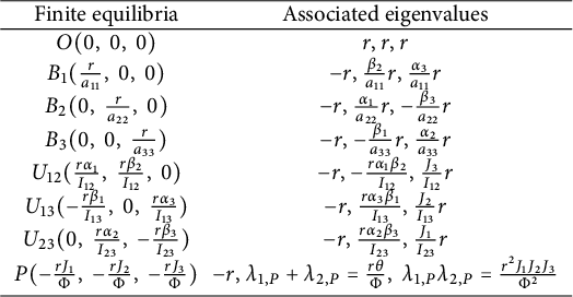
As we can check, besides the positive one, system (1.3) possesses at most seven other finite equilibria, all of them are boundary ones. Table 1 lists all these equilibria together with their eigenvalues.
Finite equilibria with associated eigenvalues for system (1.3).

Table 1: Long description
The table contains two columns: Finite equilibria and Associated eigenvalues.
* Row 1: Equilibrium O (0, 0, 0) with eigenvalues r, r, r.
* Row 2: Equilibrium B sub 1 (r all over a sub 11, 0, 0) with eigenvalues negative r, (beta sub 2 all over a sub 11) r, and (alpha sub 3 all over a sub 11) r.
* Row 3: Equilibrium B sub 2 (0, r all over a sub 22, 0) with eigenvalues negative r, (alpha sub 1 all over a sub 22) r, and minus (beta sub 3 all over a sub 22) r.
* Row 4: Equilibrium B sub 3 (0, 0, r all over a sub 33) with eigenvalues negative r, minus (beta sub 1 all over a sub 33) r, and (alpha sub 2 all over a sub 33) r.
* Row 5: Equilibrium U sub 12 (r alpha sub 1 all over I sub 12, r beta sub 2 all over I sub 12, 0) with eigenvalues negative r, minus (r alpha sub 1 beta sub 2 all over I sub 12), and (J sub 3 all over I sub 12) r.
* Row 6: Equilibrium U sub 13 (minus r beta sub 1 all over I sub 13, 0, r alpha sub 3 all over I sub 13) with eigenvalues negative r, (r alpha sub 3 beta sub 1 all over I sub 13), and (J sub 2 all over I sub 13) r.
* Row 7: Equilibrium U sub 23 (0, r alpha sub 2 all over I sub 23, minus r beta sub 3 all over I sub 23) with eigenvalues negative r, (r alpha sub 2 beta sub 3 all over I sub 23), and (J sub 1 all over I sub 23) r.
* Row 8: Equilibrium P (minus r J sub 1 all over Phi, minus r J sub 2 all over Phi, minus r J sub 3 all over Phi) with eigenvalues negative r and a system where lambda sub 1,P plus lambda sub 2,P equals r theta all over Phi, and lambda sub 1,P times lambda sub 2,P equals r-squared J sub 1 J sub 2 J sub 3 all over Phi-squared.
It is verified that the three coordinate planes are invariant for the Lotka–Volterra system (1.3) in
$\mathbb {R}^{3}_{+}$
 , and that restricted to each one of them system (1.3) becomes a two-dimensional cooperative or competitive system. So it follows from Theorem 2.3 in [Reference Hirsch3] and its proof that every trajectory is eventually monotone. Therefore, one gets the following proposition.
Proposition System (1.3) has no a periodic orbit in each invariant coordinate plane.
3.2 Dynamics at infinity
In this subsection, we shall study the dynamics of system (1.3) at infinity by the Poincaré compactification.
Firstly, we study the equilibria at infinity in the positive
${x_1}$
 direction. Taking the change of variables

or equivalently

and the time rescaling

system (1.3) is transformed into

Direct calculations show that system (3.2) has at most four equilibria in the invariant plane at infinity, i.e., the
$({u_1},{v_1})$
 plane (
$w_{1}=0$
 ). The three equilibria on the axes (if exist) are
$A_{1}:=(0,\;0,\;0)$
 ,
$V_{12}:=( \beta _2/\alpha _1,\;0,\;0)$
 and
$V_{13}:=(0, \; -\alpha _3/\beta _1,\;0)$
 , where
$A_{1}$
 is at the positive endpoint of the
$x_{1}$
 -axis,
$V_{12}$
 is at the positive endpoint of the line
$\{x_{2}=\frac {\beta _{2}}{\alpha _{1}}x_{1}\}\cap \{x_{3}=0\}$
 , and
$V_{13}$
 is at the positive endpoint of the line
$\{x_{3}=-\frac {\alpha _{3}}{\beta _{1}}x_{1}\}\cap \{x_{2}=0\}$
 . The eigenvalues of system (3.2) at
$A_{1}$
 are
$\beta _{2}$
 ,
$\alpha _{3}$
 and
$a_{11}$
 , the first two have the eigenvectors tangent to the plane at infinity, and the third one has the eigenvector pointing to the finite space. The eigenvalues of system (3.2) at
$V_{12}$
 are
$-\beta _{2}$
 ,
$J_{3}/\alpha _{1}$
 and
$I_{12}/\alpha _{1}$
 , the first two have the eigenvectors tangent to the plane at infinity and the third one has the eigenvector pointing to the finite space. The eigenvalues of system (3.2) at
$V_{13}$
 are
$-\alpha _{3}$
 ,
$-J_{2}/\beta _{1}$
 and
$-I_{13}/\beta _{1}$
 , the first two have the eigenvectors tangent to the plane at infinity and the third one has the eigenvector pointing to the finite space. The fourth equilibrium (if exists) is a positive one in the
$({u_1},{v_1})$
 plane, and it must be
$Q:=(J _2/J _1,\;J _3/J _1,\;0)$
 , which is at the positive endpoint of the line
$\{x_{2}=\frac {J_{2}}{J_{1}}x_{1}\}\cap \{x_{3}=\frac {J_{3}}{J_{1}}x_{1}\}$
 . Let
$\lambda _{1,Q}, \ \lambda _{2,Q}$
 and
$\lambda _{3,Q}$
 be the three eigenvalues. They must satisfy


Next we will study the equilibria at infinity in the positive
${x_2}$
 direction. Taking the change of the variables

or equivalently

and the time rescaling

system (1.3) can be written as

Now we try to figure out the possible equilibria of system (3.3) on the
${v_2}$
 -axis, because the other equilibria at infinity were studied through the previous investigation. The possible equilibria of system (3.3) on the
${v_2}$
 -axis are
$A_{2}:=(0,\;0,\;0)$
 and
$V_{23}:=(0,\; - \beta _3/\alpha _2,\;0)$
 . The former is at the positive endpoint of the
$x_{2}$
 -axis and the latter is at the positive endpoint of the line
$\{x_{3}=-\frac {\beta _{3}}{\alpha _{2}}x_{2}\}\cap \{x_{1}=0\}$
 . The eigenvalues of system (3.3) at
$A_{2}$
 are
$\alpha _{1}$
 ,
$-\beta _{3}$
 , and
$a_{22}$
 , the first two have the eigenvectors tangent to the plane at infinity, and the third one has the eigenvector pointing to the finite space. The eigenvalues of system (3.3) at
$V_{23}$
 are
$\beta _{3}$
 ,
$J_{1}/\alpha _{2}$
 , and
$I_{23}/\alpha _{2}$
 , the first two have the eigenvectors tangent to the plane at infinity and the third one has the eigenvector pointing to the finite space.
For the equilibria at infinity in the positive
${x_3}$
 direction, the change of the variables

or equivalently

and the time rescaling
$ dt = {w_3}d\tau $
 send system (1.3) to

According to the analysis to systems (3.2) and (3.3), we only need to study the equilibrium at the positive endpoint of the
$x_{3}$
 -axis, denoted by
$A_3$
 , which is the origin of system (3.4). The eigenvalues of system (3.4) at
$A_{3}$
 are
$-\beta _{1}$
 ,
$\alpha _{2}$
 , and
$a_{33}$
 , the first two have the eigenvectors tangent to the plane at infinity and the third one has the eigenvector pointing to the finite space.
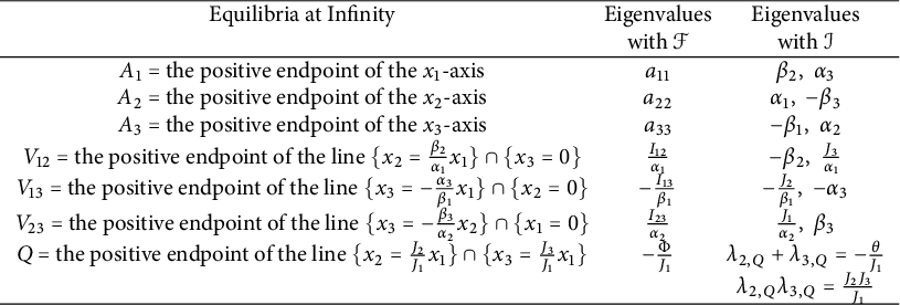
Table 2 summarizes the above results on equilibria at infinity with their associated eigenvalues. In order to obtain further information on the flow near infinity, our first result excludes the existence of limit cycles at infinity when
$\theta \neq 0$
 . Recall that
$\theta :={\beta _1}{\beta _2}{\beta _3} + {\alpha _1}{\alpha _2}{\alpha _3}$
 determines whether the two eigenvalues
$\lambda _{2,Q}$
 and
$\lambda _{3,Q}$
 of the positive equilibrium Q at infinity are a pair of pure imaginary numbers.
Equilibria at Infinity and their associated eigenvalues of system (1.3).
$\mathcal F=$
 its eigenvector pointing to the finite space,
$\mathcal I=$
 their eigenvectors tangent to the plane at the infinity.

Table 2: Long description
The table consists of three main columns.
* Row 1: Equilibria A sub 1 (positive endpoint of x sub 1 axis) has eigenvalues a sub 11 and beta sub 2, alpha sub 3.
* Row 2: Equilibria A sub 2 (positive endpoint of x sub 2 axis) has eigenvalues a sub 22 and alpha sub 1, minus beta sub 3.
* Row 3: Equilibria A sub 3 (positive endpoint of x sub 3 axis) has eigenvalues a sub 33 and minus beta sub 1, alpha sub 2.
* Row 4: Equilibria V sub 12 (intersection of x sub 2 equals beta sub 2 over alpha sub 1 times x sub 1 and x sub 3 equals 0) has eigenvalues I sub 12 over alpha sub 1 and minus beta sub 2, J sub 3 over alpha sub 1.
* Row 5: Equilibria V sub 13 (intersection of x sub 3 equals minus alpha sub 3 over beta sub 1 times x sub 1 and x sub 2 equals 0) has eigenvalues minus I sub 13 over beta sub 1 and minus J sub 2 over beta sub 1, minus alpha sub 3.
* Row 6: Equilibria V sub 23 (intersection of x sub 3 equals minus beta sub 3 over alpha sub 2 times x sub 2 and x sub 1 equals 0) has eigenvalues I sub 23 over alpha sub 2 and J sub 1 over alpha sub 2, beta sub 3.
* Row 7: Equilibria Q (intersection of x sub 2 equals J sub 2 over J sub 1 times x sub 1 and x sub 3 equals J sub 3 over J sub 1 times x sub 1) has eigenvalues minus Phi over J sub 1 and a sum lambda sub 2,Q plus lambda sub 3,Q equals minus theta over J sub 1.
* Row 8: Final entry for Equilibria Q provides the product lambda sub 2,Q times lambda sub 3,Q equals J sub 2 times J sub 3 over J sub 1.
Proposition The compactified vector field associated with system (1.3) has no a periodic orbit on
$\Sigma ^{\infty }_{+}$
 when
$\theta \neq 0$
 .
Proof Nonexistence of periodic orbits of system (1.3) at infinity when
$\theta \neq 0$
 is equivalent to the fact that the two-dimensional Lotka–Volterra system

does not possess any periodic orbit in the first quadrant when
$\theta \neq 0$
 . The last argument can be verified by (3.2) via the Bendixson criterion together with the transformation
$u=\ln u_1$
 and
$v=\ln v_1$
 .
The next result characterizes the invariant lines of system (1.3).
Proposition System (1.3) has invariant lines under the next cases.
-
(a) If the positive equilibrium $Q $
at infinity exists, then
$\Gamma =\left \{{(s, \frac {J_{2}}{J_{1}}s, \frac {J_{3}}{J_{1}}s): s\geq 0}\right \}$
is an invariant line. -
(b) If the equilibrium ${V_{13}}$
at infinity exists, then
$\Gamma _{13}=\left \{(s, 0, -\frac {\alpha _{3}}{\beta _{1}}s): s\geq 0\right \}$
is an invariant line. If the equilibrium
${V_{23}}$
at infinity exists, then
$\Gamma _{23}=\Big \{(0, s, -\frac {\beta _{3}}{\alpha _{2}}s): s\geq 0\Big \}$
and
$\Gamma _{12}=\left \{(s, \frac {\beta _{2}}{\alpha _{1}}s, 0): s\geq 0\right \}$
are two invariant lines.







Proof (a) If
$x(0)=(x_{1}(0), x_{2}(0), x_{3}(0))\in \Gamma $
 , then
$x(0)=(\xi , \frac {J_{2}}{J_{1}}\xi , \frac {J_{3}}{J_{1}}\xi )$
 for some
$\xi \geq 0$
 . Let
$\phi (t)$
 satisfy
$\phi ^{'}(t)=\phi (t)(r+\frac {\Phi }{J_{1}}\phi (t)), \phi (0)=\xi $
 . It follows from the expression (3.1) that
$\varphi (t)=(\phi (t), \frac {J_{2}}{J_{1}}\phi (t), \frac {J_{3}}{J_{1}}\phi (t))$
 satisfies (1.3), and so
$\Gamma $
 is invariant.
(b) If
$x(0)=(x_{1}(0), 0, x_{3}(0))\in \Gamma _{13}$
 , then
$x(0)=(\xi , 0, -\frac {\alpha _{3}}{\beta _{1}}\xi )$
 for some
$\xi \geq 0$
 . Let
$\phi (t)$
 satisfy
$\phi ^{'}(t)=\phi (t)(r+\frac {I_{13}}{\beta _{1}}\phi (t)), \phi (0)=\xi $
 . Then
$\varphi (t)=(\phi (t), 0, -\frac {\alpha _{3}}{\beta _{1}}\phi (t))$
 satisfies (1.3), and so
$\Gamma _{13}$
 is invariant. The similar arguments apply to the proofs on invariance of the lines
$\Gamma _{23}$
 and
$\Gamma _{12}$
 .
4 The Lotka–Volterra system and replicator dynamics
In this section, we first introduce the relation between the Lotka–Volterra system (1.3) and its replicator equations, and then classify the global dynamics of system (1.3) by means of the dynamics of the replicator equations defined on the standard probability simplex

Set
$x=(x_{1},\ x_{2},\ x_{3})\ne 0$
 and
$y=(y_{1},\ y_{2},\ y_{3})$
 . By the transformation

system (1.3) can be transformed to

Note that
$x_{1}+x_{2}+x_{3}>0$
 , so after time rescaling one obtains the so-called replicator equations on
$S_{3}$


According to Hofbauer and Sigmund [Reference Hofbauer and Sigmund4, Theorem 7.5.1], by the change of variables

and time rescaling, system (4.2) on
$S_3\backslash \{y_3=0\}$
 is equivalent to the following two-dimensional Lotka–Volterra system in
$\mathbb {R}_{+}^2$


System (4.4) may have the four finite equilibria:

The eigenvalues at
$C_{3}$
 are
$-\beta _{1}$
 and
$\alpha _{2}$
 ; at
$M_{13}$
 are
$\beta _{1}$
 and
$J_{2}/\alpha _{3} $
 ; at
$M_{23}$
 are
$-J_{1}/\beta _{3}$
 and
$-\alpha _{2}$
 ; and at N are
$\lambda _{1}$
 and
$\lambda _{2}$
 , which satisfy

To know the properties of the equilibria at infinity for system (4.4), we make the transformation

to system (4.4), and get the system

System (4.5) on
${\overline {w}_2}=0$
 may have the two equilibria
$C_{1}:=(0,\;0)$
 and
$M_{12}:=\left ( \frac {{{\beta _2}}}{{{\alpha _1}}},\;0\right )$
 , whose eigenvalues are respectively
$\beta _{2}$
 and
$\alpha _{3}$
 , and
$-\beta _{2}$
 and
$J_{3}/\alpha _{1}$
 . The former is at the positive endpoint of the
$\widetilde {y}_{1}$
 -axis and the latter is at the positive endpoint of the line
$\widetilde {y}_{2}=\frac {\beta _{2}}{\alpha _{1}}\widetilde {y}_{1}$
 .
The equilibrium at the endpoint of the positive
$\widetilde y_2$
 -axis can be studied by the system

which is obtained from system (4.4) via the transformation

The equilibrium at the origin of system (4.6), denoted by
$C_{2}$
 , has the eigenvalues
$\alpha _1$
 and
$-\beta _3$
 .
The above analysis shows that the dynamics of system (4.2) on
$S_{3}$
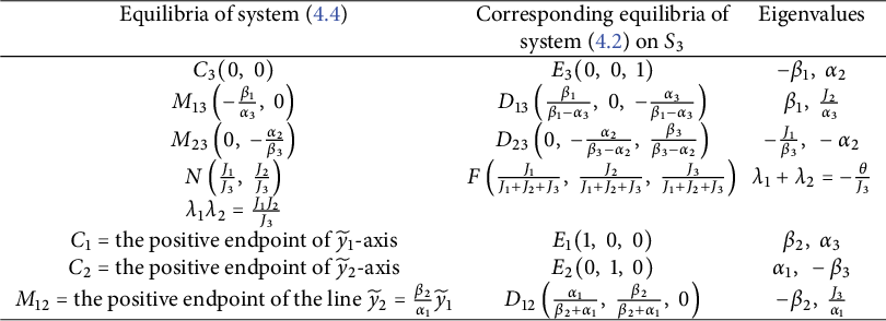
 is topologically equivalent to that of system (4.4) together with infinity. This result is helpful to investigate the global dynamics of system (1.3). Table 3 summarizes the information about the finite equilibria and the equilibria at infinity of system (4.4) together with their corresponding equilibria of system (4.2) on
$S_{3}$
 .
Equilibria with associated eigenvalues of system (4.2) on
$S_{3}$
 .

Table 3: Long description
The table consists of three main columns: Equilibria of system 4.4, Corresponding equilibria of system 4.2 on S sub 3, and Eigenvalues.
* Row 1: C sub 3 (0, 0) corresponds to E sub 3 (0, 0, 1) with eigenvalues minus beta sub 1, alpha sub 2.
* Row 2: M sub 13 (minus beta sub 1 all over alpha sub 3, 0) corresponds to D sub 13 (beta sub 1 all over beta sub 1 minus alpha sub 3, 0, minus alpha sub 3 all over beta sub 1 minus alpha sub 3) with eigenvalues beta sub 1, J sub 2 all over alpha sub 3.
* Row 3: M sub 23 (0, minus alpha sub 2 all over beta sub 3) corresponds to D sub 23 (0, minus alpha sub 2 all over beta sub 3 minus alpha sub 2, beta sub 3 all over beta sub 3 minus alpha sub 2) with eigenvalues minus J sub 1 all over beta sub 3, minus alpha sub 2.
* Row 4: N (J sub 1 all over J sub 3, J sub 2 all over J sub 3) corresponds to F (J sub 1 all over J sub 1 plus J sub 2 plus J sub 3, J sub 2 all over J sub 1 plus J sub 2 plus J sub 3, J sub 3 all over J sub 1 plus J sub 2 plus J sub 3). The eigenvalues are defined by two equations: lambda sub 1 plus lambda sub 2 equals minus theta all over J sub 3, and lambda sub 1 lambda sub 2 equals J sub 1 J sub 2 all over J sub 3.
* Row 5: C sub 1, defined as the positive endpoint of the y-tilde sub 1-axis, corresponds to E sub 1 (1, 0, 0) with eigenvalues beta sub 2, alpha sub 3.
* Row 6: C sub 2, defined as the positive endpoint of the y-tilde sub 2-axis, corresponds to E sub 2 (0, 1, 0) with eigenvalues alpha sub 1, minus beta sub 3.
* Row 7: M sub 12, defined as the positive endpoint of the line y-tilde sub 2 equals beta sub 2 all over alpha sub 1 times y-tilde sub 1, corresponds to D sub 12 (alpha sub 1 all over beta sub 2 plus alpha sub 1, beta sub 2 all over beta sub 2 plus alpha sub 1, 0) with eigenvalues minus beta sub 2, J sub 3 all over alpha sub 1.
By the transformation (4.1), we obtain

Suppose that
$\Lambda $
 is an orbit of system (4.2). Let
$\mathcal {C}=\mathcal {C}(\Lambda )$
 be the cone generated by the moving ray which passes through the origin and a moving point on the orbit
$\Lambda $
 . We call
$\Lambda $
 the directrix of the cone
$\mathcal {C}$
 . From the transformation (4.1) and the uniqueness of solution of system (4.2) with respect to the initial condition, it follows that
$\mathcal {C}$
 is invariant under the flow of system (1.3), and that every solution of system (1.3) on
$\mathcal {C}$
 has the projection
$\Lambda $
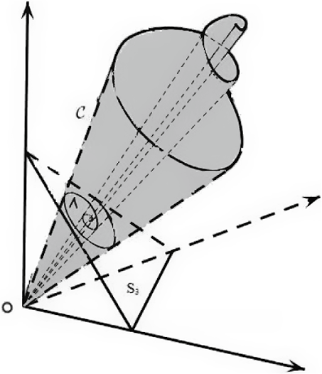
 via (4.1). Such a corresponding relation is illustrated in Figure 1. Therefore, the asymptotic behaviors of the orbits of system (1.3) can be obtained by those of system (4.2) on
$S_{3}$
 . In addition, one can check through Proposition 3.3 that
$\{O,\ U_{12},\ V_{12},\ D_{12}\}\subset \Gamma _{12}$
 ,
$\{O,\ U_{13},\ V_{13},\ D_{13}\}\subset \Gamma _{13}$
 ,
$\{O,\ U_{23},\ V_{23},\ D_{23}\}\subset \Gamma _{23}$
 , and
$\{O,\ P,\ Q,\ F\}\subset \Gamma $
 , which provide the existence of the considered equilibria as mentioned previously.
The picture on the cone
$\mathcal {C}$
 with the directrix
$\Lambda $
 and the projection from a solution of system (1.3) on
$\mathcal {C}$
 to the orbit
$\Lambda $
 of system (4.2) via (4.1).

Figure 1 Long description
The diagram is set in a three-dimensional space with three axes originating from a point labeled O.
* At the origin O, a solid black line and a dashed line extend to the right, while a solid black line extends vertically.
* A shaded cone, labeled script C, extends diagonally upward from the origin.
* Inside the cone, a central axis is represented by dashed lines.
* A spiral curve originates near the base of the cone and winds upward around the central axis.
* An elliptical cross-section within the cone contains a smaller spiral labeled Lambda.
* A triangular plane labeled S sub 3 is positioned below the cone, intersecting the horizontal axes.
* Dashed lines indicate projections from the spiral on the surface of the cone down toward the directrix Lambda and the plane S sub 3.
Similar to the proof of Proposition 3.2, we have


5 Dynamics of the replicator equations
The conditions
$a_{ij}>0$
 force that
$\alpha _{1}>0$
 and
$\beta _{2}>0$
 , so the equilibrium
$V_{12}$
 at infinity must exist. The next classification on the global dynamics of system (1.3) relies on the signs of the terms
$\alpha _{2},~\alpha _{3},~\beta _{1},~\beta _{3},~J_{1},~J_{2},~J_{3}$
 , and
$I_{12}$
 . Firstly, we discuss how the signs of
$\alpha _{2},~\alpha _{3},~\beta _{1},$
 and
$\beta _{3}$
 affect the existence of
$V_{13}$
 and
$V_{23}$
 . Secondly, according to the signs of
$\alpha _{2},~\alpha _{3},~\beta _{1}$
 , and
$\beta _{3}$
 we further determine the signs of
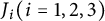
$J_{i}(i=1, 2, 3)$
 . For example, if the signs of
$\alpha _{3}$
 and
$\beta _{1}$
 are opposite, then the equilibria
$U_{13}$
 and
$V_{13}$
 both exist, so we need to discuss the sign of
$J_{2}$
 . If the signs of
$\alpha _{2}$
 and
$\beta _{3}$
 are opposite, then the equilibria
$U_{23}$
 and
$V_{23}$
 both exist, so we further discuss the sign of
$J_{1}$
 . Since the equilibrium
$V_{12}$
 at infinity always exist, we need to discuss the sign of
$J_{3}$
 for each of the cases. Of course, in the case that the signs of
$\alpha _{2},~\alpha _{3},~\beta _{1}$
 , and
$\beta _{3}$
 are determined,
$J_{1},~J_{2}$
 or
$J_{3}$
 are also determined, then it is not necessary to discuss their signs. Lastly, we will discuss the sign of
$I_{12}$
 to determine whether the equilibrium
$U_{12}$
 exists. All the possibilities in logic of the three-dimensional type-K monotone Lotka–Volterra system (1.3) are listed in Table 4.
All the possibilities in logic of the three-dimensional type-K monotone Lotka–Volterra system (1.3). For the empty entries in the table, their signs either are uniquely determined by the signs of
$\alpha _{2},~\alpha _{3},~\beta _{1}$
 and
$\beta _{3}$
 , or do not affect the stability of the equilibria.

Table 4: Long description
The table consists of 9 columns: Case, alpha sub 2, alpha sub 3, beta sub 1, beta sub 3, J sub 1, J sub 2, J sub 3, and I sub 12.
* Cases 1 through 31: All entries in the I sub 12 column are positive (+).
* Cases 32 through 62: All entries in the I sub 12 column are less than or equals 0.
Key parameter distributions include:
* Case 1: alpha sub 2, alpha sub 3, beta sub 1, and beta sub 3 are all positive (+). J columns are empty.
* Cases 2 and 3: alpha sub 2 is negative (-), while alpha sub 3, beta sub 1, and beta sub 3 are positive (+). J sub 1 is positive (+) in Case 2 and negative (-) in Case 3.
* Cases 10 through 13: alpha sub 2 and alpha sub 3 are negative (-), while beta sub 1 and beta sub 3 are positive (+). J sub 1 and J sub 2 vary between positive and negative signs.
* Cases 26 through 29: alpha sub 2, beta sub 1, and beta sub 3 are negative (-), while alpha sub 3 is positive (+). J sub 2 and J sub 3 vary between positive and negative signs.
* Case 31 and 62: All primary parameters (alpha sub 2, alpha sub 3, beta sub 1, beta sub 3) are negative (-).
Empty cells in the J sub 1, J sub 2, and J sub 3 columns indicate values that are either uniquely determined by the alpha and beta signs or do not affect the stability of the equilibria.
The total 35 global topological dynamical classes of the compactified vector fields for the three-dimensional type-K monotone Lotka–Volterra system (1.3) in R. The notations
$\bullet $
 and
$ \circ $
 denote an attractor and a repeller in R respectively, while a saddle in R is the intersection of its stable and unstable manifolds.

Table 5: Long description
The table is titled Table 5 and contains four columns.
Column 1: Class. Lists numerical identifiers from 1 to 35.
Column 2: Parameters. Contains mathematical conditions involving alpha sub 2, alpha sub 3, beta sub 1, beta sub 3, J sub 1, J sub 2, J sub 3, and I sub 12. For example, Class 1 is defined by alpha sub 2 > 0, alpha sub 3 > 0, beta sub 1 > 0, beta sub 3 > 0, and I sub 12 > 0.
Column 3: Phase portraits of (4.2) on S sub 3. Displays two-dimensional triangular diagrams representing the flow on the invariant surface. Vertices are labeled E sub 1, E sub 2, and E sub 3. Solid bullets denote attractors, open rings denote repellers, and arrows indicate the direction of the vector field flow along edges and through the interior. Points like D sub 12, D sub 23, D sub 13, and F represent various equilibrium points.
Column 4: Global phase portraits in R. Displays three-dimensional diagrams of the compactified vector fields in the positive octant. These diagrams show the trajectories of the system in space, illustrating how they converge toward attractors or move away from repellers within the bounded region.
The table continues through 35 distinct classes, each representing a unique topological configuration of the dynamical system based on the specified parameter ranges.
Next we study the dynamics of system (4.2) on
$S_{3}$
 according to the cases in Table 4 one by one. We notice that the Poincaré–Bendixson theorem holds on
$S_{3}$
 , and by Table 3 that system (4.2) on
$S_{3}$
 has always the equilibria
$E_{i}~(i=1, 2, 3)$
 and
$D_{12}$
 . Moreover, one can check that the equilibrium
$D_{23}$
 exists if and only if
$\alpha _{2}$
 and
$\beta _{3}$
 have opposite signs, and that the equilibrium
$D_{13}$
 exists if and only if
$\alpha _{3}$
 and
$\beta _{1}$
 have opposite signs.
Cases 1 and 32. According to the signs of
$\alpha _{i}~(i=1, 2, 3)$
 and
$\beta _{j}~(j=1, 2, 3)$
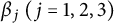 , one has
$J_{1}=\alpha _{1}\alpha _{2}+\beta _{1}\beta _{3}+\alpha _{2}\beta _{3}>0$
 and
$J_{3}=\alpha _{1}\alpha _{3}-\beta _{2}\beta _{3}-\alpha _{1}\beta _{2}=-\beta _{2}\beta _{3}-\alpha _{1}(a_{31}+a_{21})<0.$
 These imply that system (4.2) on
$S_{3}$
 has no the positive equilibrium F, and so has no a nontrivial periodic orbit. By Table 3, one can verify that
$E_{2}$
 and
$E_{3}$
 are saddles,
$D_{12}$
 is an attractor, and
$E_{1}$
 is a repeller. So the global phase portraits of system (4.2) on
$S_{3}$
 are those in Table 5 (1a) and (18a).
Cases 2 and 33. Since
$J_{3}=\alpha _{1}\alpha _{3}-\beta _{2}\beta _{3}-\alpha _{1}\beta _{2}=-\beta _{2}\beta _{3}- \alpha _{1}(a_{31}+a_{21})<0$
 and
$J_{1}>0$
 , these cause nonexistence of the equilibrium F, and so system (4.2) on
$S_{3}$
 has no a nontrivial periodic orbit. Referring to Table 3, one gets that
$E_{3}$
 and
$D_{12}$
 are the attractors,
$E_{2}$
 and
$D_{23}$
 are saddles, and
$E_{1}$
 is a repeller. Hence the global phase portraits of system (4.2) on
$S_{3}$
 are those in Table 5 (2a) and (19a).
Cases 3 and 34. Because
$J_{1}<0$
 ,
$J_{3}=\alpha _{1}\alpha _{3}-\beta _{2}\beta _{3}-\alpha _{1}\beta _{2}=-\beta _{2}\beta _{3}-\alpha _{1}(a_{31}+a_{21})<0$
 and
$J_{2}=\alpha _{2}\alpha _{3}-\beta _{1}\beta _{2}+\alpha _{3}\beta _{1}=\alpha _{2}\alpha _{3}-\beta _{1}(a_{31}+a_{21})<0,$
 system (4.2) on
$S_{3}$
 has the equilibrium F, which is a saddle by Table 3, and so has no a nontrivial periodic orbit. Moreover, it follows from Table 3 that
$E_{3}$
 and
$D_{12}$
 are the attractors,
$E_{1}$
 and
$D_{23}$
 are repellers, and
$E_{2}$
 is a saddle. So the global phase portraits of system (4.2) on
$S_{3}$
 are those in Table 5 (3a) and (20a).
Cases 4 and 35. It follows from
$J_{1}>0$
 and
$J_{2}<0$
 that system (4.2) on
$S_{3}$
 has no the equilibrium F, and so has no a nontrivial periodic orbit. Furthermore, by the facts that
$D_{12}$
 is an attractor,
$D_{13}$
 is a repeller, and
$E_{i}~(i=1, 2, 3)$
 are saddles, it follows that the global phase portraits of system (4.2) on
$S_{3}$
 are those in Table 5 (4a) and (21a).
Cases 5 and 36.
$J_{2}=\alpha _{2}\alpha _{3}-\beta _{1}\beta _{2}+\alpha _{3}\beta _{1}=\alpha _{2}\alpha _{3}-\beta _{1}(a_{31}+a_{21})>0$
 and
$J_{3}=\alpha _{1}\alpha _{3}-\beta _{2}\beta _{3}-\alpha _{1}\beta _{2}=-\beta _{2}\beta _{3}-\alpha _{1}(a_{31}+a_{21})<0$
 force that system (4.2) on
$S_{3}$
 has no the equilibrium F, and so has no a nontrivial periodic orbit. Combining the facts that
$E_{i}~(i=1, 3)$
 are repellers,
$E_{2}$
 and
$D_{13}$
 are saddles, and
$D_{12}$
 is an attractor achieves that the global phase portraits of system (4.2) on
$S_{3}$
 are those in Table 5 (5a) and (22a).
Cases 6 and 37. By
$J_{1}>0$
 and
$J_{3}>0$
 , we have

Thus
$\theta =\beta _{1}\beta _{2}\beta _{3}+\alpha _{1}\alpha _{2}\alpha _{3}>0.$
 It follows from Proposition 4.1 that system (4.2) on
$S_{3}$
 has no a nontrivial periodic orbit. Therefore,


So there is the equilibrium F. Referring to Table 3, one can verify that F is an attractor,
$E_{1}$
 and
$E_{2}$
 are repellers, and
$E_{3}$
 ,
$D_{12}$
 and
$D_{23}$
 are saddles. So the global phase portraits of system (4.2) on
$S_{3}$
 are those in Table 5 (6a) and (23a).
Cases 8 and 39. It follows from
$J_{1}>0$
 and
$J_{3}<0$
 that system (4.2) on
$S_{3}$
 has no the equilibrium F, and so has no a nontrivial periodic orbit. The facts that
$E_{i}~(i=1, 2)$
 are repellers,
$E_{3}$
 and
$D_{23}$
 are saddles, and
$D_{12}$
 is an attractor indicate that the global phase portraits of system (4.2) on
$S_{3}$
 are those in Table 5 (7a) and (25a).
Cases 9 and 40. By
$J_{1}<0$
 and
$J_{3}<0$
 , we have

Thus
$\theta =\beta _{1}\beta _{2}\beta _{3}+\alpha _{1}\alpha _{2}\alpha _{3}<0.$
 Therefore,


So system (4.2) on
$S_{3}$
 has the equilibrium F, which is a saddle by Table 3, and so has no a nontrivial periodic orbit. In addition,
$D_{12}$
 and
$D_{23}$
 are the attractors,
$E_{i}~(i=1, 2)$
 are repellers, and
$E_{3}$
 is a saddle. By these facts it follows that the global phase portraits of system (4.2) on
$S_{3}$
 are those in Table 5 (8a) and (26a).
Cases 10 and 41. Owing to
$\theta =\beta _{1}\beta _{2}\beta _{3}+\alpha _{1}\alpha _{2}\alpha _{3}>0$
 , one has

This contradiction means that these two cases cannot be realized.
Cases 11 and 42. It follows from
$J_{1}<0$
 and
$J_{2}>0$
 that system (4.2) on
$S_{3}$
 has no the equilibrium F, and so has no a nontrivial periodic orbit. In addition,
$E_{3}$
 and
$D_{12}$
 are the attractors,
$E_{i}~(i=1, 2)$
 and
$D_{13}$
 are saddles, and
$D_{23}$
 is a repeller. By these facts it follows that the global phase portraits of system (4.2) on
$S_{3}$
 are those in Table 5 (9a) and (27a).
Cases 13 and 44. It follows from
$J_{i}<0~(i=1, 2, 3)$
 that system (4.2) on
$S_{3}$
 has the equilibrium F, which is a saddle by Table 3, and so has no a nontrivial periodic orbit. Moreover,
$E_{3}$
 and
$D_{12}$
 are the attractors,
$D_{13}$
 and
$D_{23}$
 are repellers, and
$E_{i}~(i=1, 2)$
 are saddles. It follows that the global phase portraits of system (4.2) on
$S_{3}$
 are those in Table 5 (10a) and (28a).
Cases 14 and 45. Because
$J_{2}>0$
 ,
$J_{1}=\alpha _{1}\alpha _{2}+\beta _{1}\beta _{3}+\alpha _{2}\beta _{3}<0$
 and
$J_{3}=\alpha _{1}\alpha _{3}-\beta _{2}\beta _{3}-\alpha _{1}\beta _{2}=-\beta _{2}\beta _{3}-\alpha _{1}(a_{31}+a_{21})<0,$
 system (4.2) on
$S_{3}$
 has no the equilibrium F, and so has no a nontrivial periodic orbit. Moreover,
$E_{1}$
 and
$D_{23}$
 are repellers,
$E_{i}~(i=2, 3)$
 and
$D_{13}$
 are saddles, and
$D_{12}$
 is an attractor, it follows that the global phase portraits of system (4.2) on
$S_{3}$
 are those in Table 5 (11a) and (29a).
Cases 15 and 46. It follows from
$J_{i}<0~(i=1, 2, 3)$
 that system (4.2) on
$S_{3}$
 has the equilibrium F, which is a saddle by Table 3, and so has no a nontrivial periodic orbit. Referring to Table 3,
$D_{12}$
 and
$D_{13}$
 are the attractors,
$E_{1}$
 and
$D_{23}$
 are repellers, and
$E_{i}~(i=2, 3)$
 are saddles. So the global phase portraits of system (4.2) on
$S_{3}$
 are those in Table 5 (12a) and (30a).
Cases 16 and 47. Because
$J_{1}=\alpha _{1}\alpha _{2}+\beta _{1}\beta _{3}+\alpha _{2}\beta _{3}=\beta _{1}\beta _{3}+ \alpha _{2}(a_{12}+a_{32})<0$
 and
$J_{3}>0$
 , system (4.2) on
$S_{3}$
 has no the equilibrium F, and so has no a nontrivial periodic orbit. Moreover,
$E_{3}$
 is an attractor,
$E_{i}~(i=1, 2)$
 are repellers, and
$D_{12}$
 is a saddle. It follows that the global phase portraits of system (4.2) on
$S_{3}$
 are those in Table 5 (13a) and (31a).
Cases 17 and 48. Because
$J_{3}<0$
 ,
$J_{1}=\alpha _{1}\alpha _{2}+\beta _{1}\beta _{3}+\alpha _{2}\beta _{3}=\beta _{1}\beta _{3}+\alpha _{2}(a_{12}+a_{32})<0$
 and
$J_{2}=\alpha _{2}\alpha _{3}-\beta _{1}\beta _{2}+\alpha _{3}\beta _{1}=\alpha _{2}\alpha _{3}-\beta _{1}(a_{31}+a_{21})<0,$
 system (4.2) on
$S_{3}$
 has the equilibrium F, which is a saddle, and so no a nontrivial periodic orbit. From Table 3,
$E_{3}$
 and
$D_{12}$
 are the attractors, and
$E_{i}~(i=1, 2)$
 are repellers. So the global phase portraits of system (4.2) on
$S_{3}$
 are those in Table 5 (14a) and (32a).
Cases 18 and 49. By the signs of terms
$\alpha _{i}~(i=1, 2, 3)$
 and
$\beta _{j}~(j=1, 2, 3)$
 , we have
$\theta = \beta _{1}\beta _{2}\beta _{3}+\alpha _{1}\alpha _{2}\alpha _{3}<0$
 and
$J_{3}<0$
 . Suppose that
$J_{i}<0~(i=1, 2)$
 . Then

This contradiction means that at least one of
$J_1$
 and
$J_2$
 is nonnegative. Thus system (4.2) on
$S_{3}$
 has no the equilibrium F, and so has no a nontrivial periodic orbit. In addition,
$D_{12}$
 is an attractor,
$E_{3}$
 is a repeller, and
$E_{i}~(i=1, 2)$
 are saddles. So the global phase portraits of system (4.2) on
$S_{3}$
 are those in Table 5 (15a) and (33a).
Cases 21 and 52. Because
$J_{3}>0$
 ,
$J_{1}=\alpha _{1}\alpha _{2}+\beta _{1}\beta _{3}+\alpha _{2}\beta _{3}=\beta _{1}\beta _{3}+\alpha _{2}(a_{12}+a_{32})>0$
 and
$J_{2}=\alpha _{2}\alpha _{3}-\beta _{1}\beta _{2}+\alpha _{3}\beta _{1}=\alpha _{2}\alpha _{3}-\beta _{1}(a_{31}+a_{21})>0,$
 system (4.2) on
$S_{3}$
 has the equilibrium F, and so has no a nontrivial periodic orbit. By Table 3, F is an attractor,
$E_{i}~(i=1, 2, 3)$
 are repellers, and
$D_{12}, D_{13}$
 , and
$D_{23}$
 are saddles. So the global phase portraits of system (4.2) on
$S_{3}$
 are those in Table 5 (16a) and (34a).
Cases 22 and 53. Because
$J_{3}<0$
 ,
$J_{1}=\alpha _{1}\alpha _{2}+\beta _{1}\beta _{3}+\alpha _{2}\beta _{3}=\beta _{1}\beta _{3}+\alpha _{2}(a_{12}+a_{32})>0$
 and
$J_{2}=\alpha _{2}\alpha _{3}-\beta _{1}\beta _{2}+\alpha _{3}\beta _{1}=\alpha _{2}\alpha _{3}-\beta _{1}(a_{31}+a_{21})>0,$
 system (4.2) on
$S_{3}$
 has no the equilibrium F, and so has no a nontrivial periodic orbit. By Table 3,
$D_{13}$
 and
$D_{23}$
 are saddles,
$D_{12}$
 is an attractor, and
$E_{i}~(i=1, 2, 3)$
 are repellers. So the global phase portraits of system (4.2) on
$S_{3}$
 are those in Table 5 (17a) and (35a).
Case 38. It follows from
$J_{1}<0$
 and
$J_{3}>0$
 that system (4.2) on
$S_{3}$
 has no the equilibrium F, and so has no a nontrivial periodic orbit. By Table 3,
$D_{23}$
 is an attractor,
$E_{i}~(i=1, 2)$
 are the repellers, and
$E_{3}$
 and
$D_{12}$
 are saddles. So the global phase portrait of system (4.2) on
$S_{3}$
 is that in Table 5 (24a).
For the remaining cases, each of them is the same as one of the above cases by a permutation of the coordinates, and so the details are omitted. Table 5 illustrates all the phase portraits of system (4.2) on
$S_{3}$
 modulo permutation of the indices.
From the previous analysis arrives the next result.
Proposition Suppose that (H) holds. System (1.3) has no a nontrivial periodic orbit in
$\mathbb {R}^{3}_{+}$
 .
Having the above preparation, we can prove our main results, i.e., Theorem 2.1–Theorem 2.8.
6 Proofs of the main results
In this section, we shall prove Theorems 2.1–2.9, which classify global topological dynamics of the three-dimensional type-K monotone Lotka–Volterra system (1.3) in R via the Poincaré compactification. Suppose that E is an equilibrium of the compactified vector field associated with system (1.3) restricted to R, and that
$\varphi _{t}(x)$
 is the solution of this vector field such that
$\varphi _{0}(x)=x$
 . In order to better describe the global dynamics of the system, set


By Tables 1 and 2, one gets that system (1.3) has always the finite equilibria
$O, B_{i}~(i=1, 2, 3)$
 and the equilibria at infinity
$A_{j}~(j=1, 2, 3)$
 and
$V_{12}$
 . Moreover, the equilibrium O is always a repeller, and
$B_{i}~(i=1, 2)$
 are always saddles. It follows from Proposition 5.1 that system (1.3) does not possess any nontrivial periodic orbits in
$\mathbb {R}^{3}_{+}$
 . If
$I_{12}>0$
 then there is the equilibrium
$U_{12}$
 ; if
$\alpha _{3}>0$
 (resp.
$\alpha _{3}<0$
 ) and
$\beta _{1}<0$
 (resp.
$\beta _{1}>0$
 ) then it follows from
$I_{13}=-a_{11}\beta _{1}+a_{13}\alpha _{3}>0$
 (resp.
$I_{13}<0$
 ) that there are the equilibria
$U_{13}$
 and
$V_{13}$
 ; and if
$\alpha _{2}>0$
 (resp.
$\alpha _{2}<0$
 ) and
$\beta _{3}<0$
 (resp.
$\beta _{3}>0$
 ) then it follows from
$I_{23}=a_{22}\alpha _{2}-a_{23}\beta _{3}>0$
 (resp.
$I_{23}<0$
 ) that there are the equilibria
$U_{23}$
 and
$V_{23}$
 . If
$I_{12}\leq 0$
 , the equilibrium
$U_{12}$
 disappears; if
$\alpha _{3}$
 and
$\beta _{1}$
 have same signs, the equilibria
$U_{13}$
 and
$V_{13}$
 disappear; and if
$\alpha _{2}$
 and
$\beta _{3}$
 have same signs, the equilibria
$U_{23}$
 and
$V_{23}$
 disappear. Suppose that
$J_{i}>0$
 (resp.
$J_{i}<0$
 ) for
$i=1, 2, 3$
 , the equilibria P and Q exist, because
$ \Phi =-a_{31}{J _1}-a_{32}{J _2}-a_{33}{J _3}<0$
 (resp.
$\Phi>0$
 ). According to the analysis in Section 5, we only need to discuss the following 35 cases. After completing the analysis on these cases we can finish the proofs of our main results.
Case 1. It follows from
$J_{1}>0$
 and
$J_{3}<0$
 that the equilibria P and Q do not exist. By Tables 1 and 2,
$U_{12}$
 is an attractor,
$A_{1}$
 is a repeller, and
$A_{i}~(i=2, 3)$
 ,
$B_{3}$
 and
$V_{12}$
 are saddles. By the Poincaré–Bendixson theorem and the invariance of the considered planes, we can obtain the phase portraits on
$\Sigma _+^{\infty }$
 ,
$p(x_{1}=0)\cap R, \ p(x_{2}=0)\cap R$
 and
$ p(x_{3}=0)\cap R $
 , which are shown in Table 5
$(1b)$
 .
Any orbit in the interior of the domain limited by
$p(x_{i}=0)~(i=1, 2, 3)$
 and
$W^{u}(p(B_{1}))$
 emanates from O and tends toward
$p(U_{12})$
 . Any orbit in the interior of the domain limited by
$p(x_{j}=0)~(j=1, 2, 3)$
 ,
$\Sigma ^{\infty }_{+}$
 and
$ W^{u}(p(B_{1}))$
 emanates from
$p(A_{1})$
 and tends toward
$p(U_{12})$
 . The equilibrium
$p(U_{12})$
 is the global attractor in
$\mathrm {Int}R$
 . These facts imply that the global phase portrait in R is that in Table 5
$(1b)$
 .
Case 2. It follows from
$J_{1}>0$
 and
$J_{3}<0$
 that the equilibria P and Q do not exist. By Tables 1 and 2, it follows that
$B_{3}$
 and
$U_{12} $
 are the attractors,
$A_{1}$
 is a repeller, and
$A_{i}~(i=2, 3)$
 ,
$U_{23}$
 ,
$V_{12}$
 and
$V_{23}$
 are saddles. By the Poincaré–Bendixson theorem and the invariance of the considered planes, we can get the phase portraits on
$\Sigma _+^{\infty }$
 ,
$p(x_{1}=0)\cap R, \ p(x_{2}=0)\cap R$
 and
$ p(x_{3}=0)\cap R $
 , which are those indicated in Table 5
$(2b)$
 .
Let
$\zeta _{23}$
 be the orbit of system (4.2) which emanates from
$E_{1}$
 and tends toward
$D_{23}$
 . From the invariance of the cone
$p\left (\mathcal {C}(\zeta _{23})\right )$
 , it follows that the intersection of
$\overline {p\left (\mathcal {C}(\zeta _{23})\right )}$
 and
$\Sigma ^{\infty }_{+}$
 consists of
$p(A_{1})$
 ,
$p(V_{23})$
 and the orbit connecting
$p(A_{1})$
 and
$p(V_{23})$
 . By the transformation (4.1), any orbit of the compactified vector field of system (1.3) on the cone
$p\left (\mathcal {C}(\zeta _{23})\right )$
 must originate from the
$x_{1}$
 -axis and tend toward
$\overline {p(\Gamma _{23})}$
 . Moreover, the intersection of the two-dimensional unstable manifold of
$p(B_{1})$
 and the cone
$p\left (\mathcal {C}(\zeta _{23})\right )$
 is an orbit, which moves away from
$p(B_{1})$
 and tends toward
$p(U_{23})$
 .
Any orbit in the interior of the domain limited by
$p(x_{i}=0)~(i=1, 3)$
 and
$W^{u}(p(B_{1}))\bigcup p(\mathcal {C}(\zeta _{23}))$
 emanates from O and tends toward
$p(U_{12})$
 . Any orbit in the interior of the domain limited by
$W^{u}(p(B_{1}))\bigcup p(\mathcal {C}(\zeta _{23}))$
 and
$p(x_{j}=0)~(j=1, 2)$
 emanates from O and tends toward
$p(B_{3})$
 . Any orbit in the interior of the domain limited by
$p(x_{j}=0)~(j=1, 3)$
 ,
$\Sigma ^{\infty }_{+}$
 and
$ W^{u}(p(B_{1}))\bigcup p(\mathcal {C}(\zeta _{23}))$
 emanates from
$p(A_{1})$
 and tends toward
$p(U_{12})$
 . Any orbit in the interior of the domain limited by
$p(x_{j}=0)~(j=1, 2)$
 ,
$\Sigma ^{\infty }_{+}$
 and
$W^{u}(p(B_{1}))\bigcup p(\mathcal {C}(\zeta _{23}))$
 emanates from
$p(A_{1})$
 and tends toward
$p(B_{3})$
 . These verify that the global phase portrait in R is that in Table 5
$(2b)$
 .
Case 3. By Tables 1 and 2, there exist the equilibria P and Q, which are saddles. Moreover,
$B_{3}$
 and
$U_{12}$
 are the attractors;
$A_{1}$
 and
$V_{23}$
 are repellers; and
$A_{i}~(i=2, 3)$
 ,
$U_{23}$
 and
$V_{12}$
 are saddles. These together with the Poincaré–Bendixson theorem and the invariance of the considered planes verify that the phase portraits on
$\Sigma _+^{\infty }$
 ,
$p(x_{1}=0)\cap R, \ p(x_{2}=0)\cap R$
 and
$p(x_{3}=0)\cap R $
 are those described in Table 5
$(3b)$
 .
Let
$\zeta _{12}$
 resp.
$\zeta _{3}$
 be the orbit of system (4.2) which originates from F and tends toward
$D_{12}$
 resp.
$E_{3}$
 . From the invariance of the cone
$p\left (\mathcal {C}(\zeta _{12})\right )$
 resp.
$p\left (\mathcal {C}(\zeta _{3})\right )$
 , it follows that the intersection of the cone
$\overline {p\left (\mathcal {C}(\zeta _{12})\right )}$
 resp.
$\overline {p\left (\mathcal {C}(\zeta _{3})\right )}$
 and
$\Sigma ^{\infty }_{+}$
 consists of
$p(Q)$
 ,
$p(V_{12})$
 (resp.
$p(A_{3})$
 ) and the orbit connecting
$p(Q)$
 and
$p(V_{12})$
 (resp.
$p(A_{3})$
 ). From the transformation (4.1), any orbit of the compactified vector field of system (1.3) on the cone
$p\left (\mathcal {C}(\zeta _{12})\right )$
 resp.
$p\left (\mathcal {C}(\zeta _{3})\right )$
 must originate from
$\overline {p(\Gamma )}$
 and tend toward
$\overline {p(\Gamma _{12})}$
 (resp. the
$x_{3}$
 -axis). Moreover, the two orbits of the compactified vector field of system (1.3) in
$\mathring W^{u}(p(P))$
 must be on the cones
$p\left (\mathcal {C}(\zeta _{12})\right )$
 and
$p\left (\mathcal {C}(\zeta _{3})\right )$
 respectively, in which one tends toward the attractor
$p(U_{12})$
 and the other approaches positively to the attractor
$p(B_{3})$
 , because there is no an orbit of system (4.2) which emanates from F in the interior of
$S_{3}$
 except
$\zeta _{12}$
 ,
$\zeta _{3}$
 and F see Table 5
$(3a)$
 . Let
$\xi _{23}$
 resp.
$\xi _{1}$
 be the orbit of system (4.2) which originates from
$D_{23}$
 resp.
$E_{1}$
 and tends toward F. From the invariance of the cone
$p\left (\mathcal {C}(\xi _{23})\right )$
 resp.
$p\left (\mathcal {C}(\xi _{1})\right )$
 , it follows that the intersection of the cone
$\overline {p\left (\mathcal {C}(\xi _{23})\right )}$
 resp.
$\overline {p\left (\mathcal {C}(\xi _{1})\right )}$
 and
$\Sigma ^{\infty }_{+}$
 consists of
$p(V_{23})$
 resp.
$p(A_{1})$
 ,
$p(Q)$
 and the orbit connecting
$p(V_{23})$
 resp.
$p(A_{1})$
 and
$p(Q)$
 . Moreover, it follows from (4.1) that any orbit of the compactified vector field of system (1.3) on the cone
$p\left (\mathcal {C}(\xi _{23})\right )$
 resp.
$p\left (\mathcal {C}(\xi _{1})\right )$
 must originate from
$\overline {p(\Gamma _{23})}$
 resp. the
$x_{1}$
 -axis and tend toward
$\overline {p(\Gamma )}$
 . The intersection of
$W^{u}(p(U_{23}))$
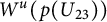 and
$p(\mathcal {C}(\xi _{23}))$
 is an orbit which emanates from
$p(U_{23})$
 and tends toward
$p(P)$
 . And the intersection of
$W^{u}(p(B_{1}))$
 and
$p(\mathcal {C}(\xi _{1})) $
 is an orbit which emanates from
$p(B_{1})$
 and tends toward
$p(P)$
 .
Further verification shows that any orbit in the interior of the domain limited by
$W^{u}(p(P)) \bigcup W^{u}(p(B_{1})) \bigcup W^{u}(p(U_{23}))\bigcup p(\mathcal {C}(\xi _{23}))\bigcup p(\mathcal {C}(\xi _{1}))\bigcup p(\Gamma )$
 and
$p(x_{j}=0)~(j=1, 3)$
 moves away from O and tends toward
$p(U_{12})$
 , and that any orbit in the interior of the domain limited by
$p(x_{j}=0)~(j=1, 2)$
 and
$ W^{u}(p(P))\bigcup W^{u}(p(B_{1}))\bigcup W^{u}(p(U_{23})) \bigcup p(\mathcal {C}(\xi _{23}))\bigcup p(\mathcal {C}(\xi _{1}))\bigcup p(\Gamma )$
 emanates from O and tends toward
$p(B_{3})$
 . Any orbit in the interior of the domain limited by
$p(\Gamma )\bigcup W^{u}(p(B_{1}))\bigcup p(\mathcal {C}(\zeta _{12}))\bigcup p(\mathcal {C}(\xi _{1}))$
 ,
$p(x_{3}=0)$
 and
$\Sigma ^{\infty }_{+}$
 emanates from
$p(A_{1})$
 and tends toward
$p(U_{12})$
 . Any orbit in the interior of the domain limited by
$p(\Gamma )\bigcup W^{u}(p(B_{1}))\bigcup p(\mathcal {C}(\zeta _{3}))\bigcup p(\mathcal {C}(\xi _{1}))$
 ,
$p(x_{2}=0)$
 and
$\Sigma ^{\infty }_{+}$
 emanates from
$p(A_{1})$
 and tends toward
$p(B_{3})$
 . Any orbit in the interior of the domain limited by
$p(\Gamma )\bigcup W^{u}(p(U_{23}))\bigcup p(\mathcal {C}(\zeta _{12})) \bigcup p(\mathcal {C}(\xi _{23}))$
 ,
$p(x_{j}=0)~(j=1, 3)$
 and
$\Sigma ^{\infty }_{+}$
 emanates from
$p(V_{23})$
 and tends toward
$p(U_{12})$
 . Any orbit in the interior of the domain limited by
$p(x_{1}=0)$
 ,
$\Sigma ^{\infty }_{+}$
 and
$p(\Gamma )\bigcup W^{u}(p(U_{23}))\bigcup p(\mathcal {C}(\zeta _{3}))\bigcup p(\mathcal {C}(\xi _{23}))$
 emanates from
$p(V_{23})$
 and tends toward
$p(B_{3})$
 . These facts show that the global phase portrait in R is that in Table 5
$(3b)$
 .
Case 4. Owing to
$J_{1}>0$
 and
$J_{i}<0~(i=2, 3)$
 , the equilibria P and Q do not exist. Referring to Tables 1 and 2, it follows that
$U_{12}$
 is an attractor,
$V_{13}$
 is a repeller, and
$B_{3} $
 ,
$U_{13}$
 ,
$V_{12}$
 and
$A_{i}~(i=1, 2, 3)$
 are saddles. It follows that the phase portraits on
$\Sigma _+^{\infty }$
 ,
$p(x_{1}=0)\cap R, \ p(x_{2}=0)\cap R$
 and
$ p(x_{3}=0)\cap R $
 are those in Table 5
$(4b)$
 .
Further verifications show that any orbit of the compactified vector field of system (1.3) passing through a point in
$W^{u}(p(U_{13}))\bigcap \mathrm {Int}R$
 will tend toward the attractor
$p(U_{12})$
 , because all orbits of system (4.2) which originate from
$D_{13}$
 in the interior of
$S_{3}$
 will tend toward
$D_{12}$
 see Table 5
$(4a)$
 . Moreover, any orbit in the interior of the domain limited by
$p(x_{j}=0)~(j=1, 2, 3)$
 and
$W^{u}(p(U_{13}))$
 emanates from O and tends toward
$p(U_{12})$
 . Any orbit in the interior of the domain limited by
$p(x_{i}=0)~(i=1, 2, 3)$
 ,
$\Sigma ^{\infty }_{+}$
 and
$ W^{u}(p(U_{13}))$
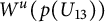 emanates from
$p(V_{13})$
 and tends toward
$p(U_{12})$
 . The equilibrium
$p(U_{12})$
 attracts all points in
$\mathrm {Int}R$
 . By these facts one gets the global phase portrait in R as that in Table 5
$(4b)$
 .
Case 5. Because of
$J_{2}>0$
 and
$J_{3}<0$
 , the equilibria P and Q do not exist. Referring to Tables 1 and 2, it follows that
$U_{12}$
 is an attractor and
$A_{i}~(i=1, 3)$
 are repellers, and
$B_{3}$
 ,
$A_{2}$
 ,
$U_{13}$
 ,
$V_{12}$
 and
$V_{13}$
 are saddles. The Poincaré–Bendixson theorem and the invariance of the considered planes further verify the phase portraits on
$\Sigma _+^{\infty }$
 ,
$p(x_{1}=0)\cap R, \ p(x_{2}=0)\cap R$
 and
$ p(x_{3}=0)\cap R $
 , which are described in Table 5
$(5b)$
 .
Let
$\zeta _{13}$
 be the orbit of system (4.2) which emanates from
$D_{13}$
 and tends toward
$D_{12}$
 . From the invariance of the cone
$p\left (\mathcal {C}(\zeta _{13})\right )$
 , it follows that the intersection of
$\overline {p\left (\mathcal {C}(\zeta _{13})\right )}$
 and
$\Sigma ^{\infty }_{+}$
 consists of
$p(V_{13})$
 ,
$p(V_{12})$
 and the orbit connecting
$p(V_{13})$
 and
$p(V_{12})$
 . Furthermore, by (4.1) one gets that any orbit of the compactified vector field of system (1.3) on the cone
$p\left (\mathcal {C}(\zeta _{13})\right )$
 must originate from
$\overline {p(\Gamma _{13})}$
 and tend toward
$\overline {p(\Gamma _{12})}$
 . Any orbit of the compactified vector field of system (1.3) passing through a point in
$\mathring W^{u}(p(U_{13}))$
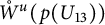 must be on the cone
$p\left (\mathcal {C}(\zeta _{13})\right )$
 and tend toward the attractor
$p(U_{12})$
 , because system (4.2) has no other orbits emanating from
$D_{13}$
 in the interior of
$S_{3}$
 except
$\zeta _{13}$
 see Table 5
$(5a)$
 .
One can further check that any orbit in the interior of the domain limited by
$p(x_{i}=0)~(i=1, 2, 3)$
 and
$W^{u}(p(B_{1}))\bigcup W^{u}(p(B_{3}))\bigcup W^{u}(p(U_{13}))$
 emanates from O and tends toward
$p(U_{12})$
 . Any orbit in the interior of the domain limited by
$p(x_{j}=0)~(j=2, 3)$
 ,
$\Sigma ^{\infty }_{+}$
 and
$W^{u}(p(B_{1}))\bigcup p(\mathcal {C}(\zeta _{13}))$
 emanates from
$p(A_{1})$
 and tends toward
$p(U_{12})$
 . The orbits in the interior of the domain limited by
$p(x_{j}=0)~(j=1, 2, 3)$
 ,
$\Sigma ^{\infty }_{+}$
 and
$W^{u}(p(B_{3}))\bigcup p(\mathcal {C}(\zeta _{13}))$
 emanate from
$p(A_{3})$
 and tend toward
$p(U_{12})$
 . The equilibrium
$p(U_{12})$
 attracts all points in
$\mathrm {Int}R$
 . So, one can obtain the global phase portrait in R as shown in Table 5
$(5b)$
 .
Case 6. It follows from
$J_{i}>0~(i=1, 2, 3)$
 and
$\Phi <0$
 that the positive finite equilibrium P and the positive equilibrium at infinity Q both exist. The former is an attractor and the latter is a saddle whose stable manifold is located in the positive plane at infinity and unstable manifold lies on the ray
$\Gamma $
 in between P and Q. By Tables 1 and 2, it follows that
$A_{i}~(i=1, 2)$
 are repellers, and that
$B_{3}$
 ,
$A_{3}$
 ,
$U_{12}$
 ,
$U_{23}$
 ,
$V_{12}$
 , and
$V_{23}$
 are saddles. These facts imply that the phase portraits on
$\Sigma _+^{\infty }$
 ,
$p(x_{1}=0)\cap R, \ p(x_{2}=0)\cap R$
 and
$ p(x_{3}=0)\cap R $
 are those in Table 5
$(6b)$
 .
For any given integer
$i\in \{1, 2\}$
 , we assume that
$\zeta _{i,i+1}$
 is the orbit of system (4.2) which originates from
$D_{i,i+1}$
 and tends toward F. The invariance of the cone
$p\left (\mathcal {C}(\zeta _{i,i+1})\right )$
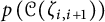 forces that the intersection of the cone
$\overline {p\left (\mathcal {C}(\zeta _{i,i+1})\right )}$
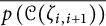 and
$\Sigma ^{\infty }_{+}$
 consists of
$p(V_{i,i+1})$
 ,
$p(Q)$
 and the orbit connecting
$p(V_{i,i+1})$
 and
$p(Q)$
 . Furthermore, by (4.1) it follows that any orbit of the compactified vector field of system (1.3) on the cone
$p\left (\mathcal {C}(\zeta _{i,i+1})\right )$
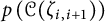 must originate from
$\overline {p(\Gamma _{i,i+1})}$
 and tend toward
$\overline {p(\Gamma )}$
 , and that any orbit of the compactified vector field of system (1.3) passing through a point in
$\mathring W^{u}(p(U_{i,i+1}))$
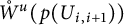 must be on the cone
$p\left (\mathcal {C}(\zeta _{i,i+1})\right )$
 and tend toward the attractor
$p(P)$
 , because system (4.2) has no any other orbit which emanates from
$D_{i,i+1}$
 in the interior of
$S_{3}$
 except
$\zeta _{i,i+1}$
 see Table 5
$(6a)$
 .
Further analysis shows that any orbit in the interior of the domain limited by
$p(x_{i}=0)~(i=1, 2, 3)$
 and
$p(P)\bigcup \bigcup \limits _{k=1}^{2}\big (W^{u}(p(B_{k})\bigcup W^{u}(p(U_{k,k+1}))\big )$
 emanates from O and tends toward
$p(P)$
 , and that any orbit in the interior of the domain limited by
$p(x_{i}=0)~(i=1, 2, 3)$
 ,
$\Sigma ^{\infty }_{+}$
 and
$p(\Gamma )\bigcup W^{u}(p(B_{1}))\bigcup \bigcup \limits _{i=1}^{2} p(\mathcal {C}(\zeta _{i,i+1}))$
 emanates from
$p(A_{1})$
 and tends toward
$p(P)$
 . Moreover, any orbit in the interior of the domain limited by
$p(\Gamma )\bigcup W^{u}(p(B_{2}))\bigcup \bigcup \limits _{i=1}^{2}p(\mathcal {C}(\zeta _{i,i+1}))$
 ,
$p(x_{j}=0)~(j=1, 3)$
 and
$\Sigma ^{\infty }_{+}$
 emanates from
$p(A_{2})$
 and tends toward
$p(P)$
 . The equilibrium
$p(P)$
 is the global attractor in
$\mathrm {Int}R$
 . These facts verify that the global phase portrait in R is that in Table 5
$(6b)$
 .
Case 8. Owing to
$J_{1}>0$
 and
$J_{3}<0$
 , the equilibria P and Q do not exist. Referring to Tables 1 and 2, it follows that
$U_{12}$
 is an attractor, and
$A_{i}~(i=1, 2)$
 are repellers, and that
$B_{3}$
 ,
$A_{3}$
 ,
$U_{23}$
 ,
$V_{12}$
 and
$V_{23}$
 are saddles. Hence, the phase portraits on
$\Sigma _+^{\infty }$
 ,
$p(x_{1}=0)\cap R, \ p(x_{2}=0)\cap R$
 and
$ p(x_{3}=0)\cap R $
 are those described in Table 5
$(7b)$
 .
Let
$\zeta _{23}$
 be the orbit of system (4.2) which emanates from
$D_{23}$
 and tends toward
$D_{12}$
 . By the invariance of the cone
$p\left (\mathcal {C}(\zeta _{23})\right )$
 , it follows that the intersection of
$\overline {p\left (\mathcal {C}(\zeta _{23})\right )}$
 and
$\Sigma ^{\infty }_{+}$
 consists of
$p(V_{23})$
 ,
$p(V_{12})$
 and the orbit connecting
$p(V_{23})$
 and
$p(V_{12})$
 . Moreover, any orbit of the compactified vector field of system (1.3) on the cone
$p\left (\mathcal {C}(\zeta _{23})\right )$
 must originate from
$\overline {p(\Gamma _{23})}$
 and tend toward
$\overline {p(\Gamma _{12})}$
 . Any orbit of the compactified vector field of system (1.3) passing through a point in
$\mathring W^{u}(p(U_{23}))$
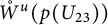 must be on the cone
$p\left (\mathcal {C}(\zeta _{23})\right )$
 and tend toward the attractor
$p(U_{12})$
 , because there are no other orbits of system (4.2) emanating from
$D_{23}$
 in the interior of
$S_{3}$
 except
$\zeta _{23}$
 see Table 5
$(7a)$
 .
Some calculations show that any orbit in the interior of the domain limited by
$p(x_{i}=0)~(i=1, 2, 3)$
 and
$\bigcup \limits _{k=1}^{2}W^{u}(p(B_{k}))\bigcup W^{u}(p(U_{23}))$
 emanates from O and tends toward
$p(U_{12})$
 , and that any orbit in the interior of the domain limited by
$p(x_{j}=0)~(j=1, 2, 3)$
 ,
$\Sigma ^{\infty }_{+}$
 and
$W^{u}(p(B_{1}))\bigcup p(\mathcal {C}(\zeta _{23}))$
 emanates from
$p(A_{1})$
 and tends toward
$p(U_{12})$
 . Moreover, any orbit in the interior of the domain limited by
$p(x_{j}=0)~(j=1, 3)$
 ,
$\Sigma ^{\infty }_{+}$
 and
$W^{u}(p(B_{2}))\bigcup p(\mathcal {C}(\zeta _{23}))$
 emanates from
$p(A_{2})$
 and tends toward
$p(U_{12})$
 . This proves that the equilibrium
$p(U_{12})$
 is the global attractor in
$\mathrm {Int}R$
 , and consequently the global phase portrait in R is that in Table 5
$(7b)$
 .
Case 9. By Tables 1 and 2, it follows that the equilibria P and Q exist and are both saddles. Moreover,
$U_{12}$
 and
$U_{23}$
 are the attractors,
$A_{i}~(i=1, 2)$
 are repellers, and
$B_{3}$
 ,
$A_{3}$
 ,
$V_{12}$
 and
$V_{23}$
 are saddles. Hence, the phase portraits on
$\Sigma _+^{\infty }$
 ,
$p(x_{1}=0)\cap R, \ p(x_{2}=0)\cap R$
 and
$ p(x_{3}=0)\cap R $
 are those in Table 5
$(8b)$
 .
For a given
$i\in \{1, 2\}$
 , let
$\zeta _{i,i+1}$
 be the orbit of system (4.2) which originates from F and tends toward
$D_{i,i+1}$
 . By the invariance of the cone
$p\left (\mathcal {C}(\zeta _{i,i+1})\right )$
 , it follows that the intersection of the cone
$\overline {p\left (\mathcal {C}(\zeta _{i,i+1})\right )}$
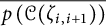 and
$\Sigma ^{\infty }_{+}$
 consists of
$p(Q)$
 ,
$p(V_{i,i+1})$
 and the orbit connecting
$p(Q)$
 and
$p(V_{i,i+1})$
 . Moreover, any orbit of the compactified vector field of system (1.3) on the cone
$p\left (\mathcal {C}(\zeta _{i,i+1})\right )$
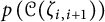 must originate from
$\overline {p(\Gamma )}$
 and tend toward
$\overline {p(\Gamma _{i,i+1})}$
 . The two orbits of the compactified vector field of system (1.3) in
$\mathring W^{u}(p(P))$
 must be on the cones
$p\left (\mathcal {C}(\zeta _{12})\right )$
 and
$p\left (\mathcal {C}(\zeta _{23})\right )$
 respectively, and one of them tends toward the attractor
$p(U_{12})$
 and the other tends toward the attractor
$p(U_{23})$
 , because there are no other orbits of system (4.2) which emanate from F in the interior of
$S_{3}$
 except
$\zeta _{12}$
 ,
$\zeta _{23}$
 , and F see Table 5
$(8a)$
 .
For a given
$k\in \{1, 2\}$
 , let
$\xi _{k}$
 be the orbit of system (4.2) which originates from
$E_{k}$
 and tends toward F. The invariance of the cone
$p\left (\mathcal {C}(\xi _{k})\right )$
 implies that the intersection of the cone
$\overline {p\left (\mathcal {C}(\xi _{k})\right )}$
 and
$\Sigma ^{\infty }_{+}$
 consists of
$p(A_{k})$
 ,
$p(Q)$
 and the orbit connecting
$p(A_{k})$
 and
$p(Q)$
 . Moreover, by (4.1) it follows that any orbit of the compactified vector field of system (1.3) on the cone
$p\left (\mathcal {C}(\xi _{k})\right )$
 must originate from the
$x_{k}$
 -axis and tend toward
$\overline {p(\Gamma )}$
 , and that the intersection of
$W^{u}(p(B_{k}))$
 and
$p(\mathcal {C}(\xi _{k}))$
 is the orbit which emanates from
$p(B_{k})$
 and tends toward
$p(P)$
 .
Further analysis shows that any orbit in the interior of the domain limited by
$p(x_{i}=0)~(i=1, 2)$
 ,
$\Sigma ^{\infty }_{+}$
 and
$p(\Gamma )\bigcup W^{u}(p(B_{1}))\bigcup p(\mathcal {C}(\zeta _{23}))\bigcup p(\mathcal {C}(\xi _{1}))$
 emanates from
$p(A_{1})$
 and tends toward
$p(U_{23})$
 , and that any orbit in the interior of the domain limited by
$p(x_{3}=0)$
 ,
$\Sigma ^{\infty }_{+}$
 and
$p(\Gamma )\bigcup W^{u}(p(B_{1}))\bigcup p(\mathcal {C}(\zeta _{12}))\bigcup p(\mathcal {C}(\xi _{1}))$
 emanates from
$p(A_{1})$
 and tends toward
$p(U_{12})$
 . For a given
$i\in \{1, 2\}$
 , each orbit in the interior of the domain limited by
$p(\Gamma )\bigcup W^{u}(p(B_{2}))\bigcup p(\mathcal {C}(\zeta _{i,i+1}))\bigcup p(\mathcal {C}(\xi _{2}))$
 ,
$p(x_{j}=0)~(j\neq i, i+1)$
 and
$\Sigma ^{\infty }_{+}$
 emanates from
$p(A_{2})$
 and tends toward
$p(U_{i,i+1})$
 . Moreover, one gets that any orbit in the interior of the domain limited by
$p(x_{3}=0)$
 and
$\bigcup \limits _{k=1}^{2}\big (W^{u}(p(B_{k}))\bigcup p(\mathcal {C}(\xi _{k}))\big ) \bigcup p(\Gamma )\bigcup W^{u}(p(P))$
 emanates from O and tends toward
$p(U_{12})$
 , and that any orbit in the interior of the domain limited by
$p(x_{i}=0)~(i= 1, 2)$
 and
$\bigcup \limits _{k=1}^{2}\big (W^{u}(p(B_{k}))\bigcup p(\mathcal {C}(\xi _{k}))\big )\bigcup p(\Gamma )\bigcup W^{u}(p(P))$
 emanates from O and tends toward
$p(U_{23})$
 . So the global phase portrait in R is that in Table 5
$(8b)$
 .
Case 11. Owing to
$J_{2}>0$
 and
$J_{i}<0~(i=1, 3)$
 , the equilibria P and Q do not exist. By Tables 1 and 2, it follows that
$B_{3}$
 and
$U_{12}$
 are the attractors,
$V_{23}$
 is a repeller, and
$U_{13}$
 ,
$U_{23}$
 ,
$V_{12}$
 ,
$V_{13}$
 and
$A_{i}~(i=1, 2, 3)$
 are saddles. Moreover, the phase portraits on
$\Sigma _+^{\infty }$
 ,
$p(x_{1}=0)\cap R, \ p(x_{2}=0)\cap R$
 and
$ p(x_{3}=0)\cap R $
 are those in Table 5
$(9b)$
 .
Let
$\zeta _{13}$
 be the orbit of system (4.2) which emanates from
$D_{23}$
 and tends toward
$D_{13}$
 . The invariance of the cone
$p\left (\mathcal {C}(\zeta _{13})\right )$
 implies that the intersection of
$\overline {p\left (\mathcal {C}(\zeta _{13})\right )}$
 and
$\Sigma ^{\infty }_{+}$
 consists of
$p(V_{23})$
 ,
$p(V_{13})$
 and the orbit connecting
$p(V_{23})$
 and
$p(V_{13})$
 . Moreover, one has that any orbit of the compactified vector field of system (1.3) on the cone
$p\left (\mathcal {C}(\zeta _{13})\right )$
 must originate from
$\overline {p(\Gamma _{23})}$
 and tend toward
$\overline {p(\Gamma _{13})}$
 . The two-dimensional stable manifold of
$p((U_{13}))$
 must be the cone
$\overline {p\left (\mathcal {C}(\zeta _{13})\right )}$
 because there are no other orbits which tend toward
$D_{13}$
 in the interior of
$S_{3}$
 except
$\zeta _{13}$
 see Table 5
$(9a)$
 .
Some calculations show that any orbit in the interior of the domain limited by
$p(x_{i}=0)~(i=1, 2, 3)$
 and
$W^{u}(p(U_{23}))\bigcup p(\mathcal {C}(\zeta _{13}))$
 emanates from O and tends toward
$p(U_{12})$
 , and that any orbit in the interior of the domain limited by
$p(x_{i}=0)~(i=1, 2)$
 and
$W^{u}(p(U_{23}))\bigcup p(\mathcal {C}(\zeta _{13}))$
 emanates from O and tends toward
$p(B_{3})$
 . Moreover, any orbit in the interior of the domain limited by
$p(x_{j}=0)~(j=1, 2, 3)$
 ,
$\Sigma ^{\infty }_{+}$
 and
$ W^{u}(p(U_{23}))\bigcup p(\mathcal {C}(\zeta _{13}))$
 emanates from
$p(V_{23})$
 and tends toward
$p(U_{12})$
 . Any orbit in the interior of the domain limited by
$p(x_{j}=0)~(j=1, 2)$
 ,
$\Sigma ^{\infty }_{+}$
 and
$ W^{u}(p(U_{23}))\bigcup p(\mathcal {C}(\zeta _{13}))$
 emanates from
$p(V_{23})$
 and tends toward
$p(B_{3})$
 . Hence, the global phase portrait in R is that in Table 5
$(9b)$
 .
Case 13. In this case, the equilibria P and Q exist and are saddles,
$B_{3}$
 and
$U_{12}$
 are the attractors,
$V_{13}$
 and
$V_{23}$
 are repellers, and
$U_{13}$
 ,
$U_{23}$
 ,
$V_{12}$
 and
$A_{i}~(i=1, 2, 3)$
 are saddles. These together with the invariance of the considered planes show that the phase portraits on
$\Sigma _+^{\infty }$
 ,
$p(x_{1}=0)\cap R, \ p(x_{2}=0)\cap R$
 and
$ p(x_{3}=0)\cap R $
 are those in Table 5
$(10b)$
 .
For a given
$i\in \{1, 2\}$
 , let
$\zeta _{i3}$
 be the orbit of system (4.2) which originates from
$D_{i3}$
 and tends toward F. The invariance of the cone
$p\left (\mathcal {C}(\zeta _{i3})\right )$
 implies that the intersection of the cone
$\overline {p\left (\mathcal {C}(\zeta _{i3})\right )}$
 and
$\Sigma ^{\infty }_{+}$
 consists of
$p(V_{i3})$
 ,
$p(Q)$
 and the orbit connecting
$p(V_{i3})$
 and
$p(Q)$
 . Moreover, any orbit of the compactified vector field of system (1.3) on the cone
$p\left (\mathcal {C}(\zeta _{i3})\right )$
 must originate from
$\overline {p(\Gamma _{i3})}$
 and tend toward
$\overline {p(\Gamma )}$
 . The intersection of
$W^{u}(p(U_{i3}))$
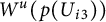 and
$p(\mathcal {C}(\zeta _{i3}))$
 is the orbit which emanates from
$p(U_{i3})$
 and tends toward
$p(P)$
 . Let
$\xi _{12}$
 resp.
$\xi _{3}$
 be the orbit of system (4.2) which originates from F and tends toward
$D_{12}$
 resp.
$E_{3}$
 . The invariance of the cone
$p\left (\mathcal {C}(\xi _{12})\right )$
 resp.
$p\left (\mathcal {C}(\xi _{3})\right )$
 means that the intersection of the cone
$\overline {p\left (\mathcal {C}(\xi _{12})\right )}$
 resp.
$\overline {p\left (\mathcal {C}(\xi _{3})\right )}$
 and
$\Sigma ^{\infty }_{+}$
 consists of
$p(Q)$
 ,
$p(V_{12})$
 resp.
$p(A_{3})$
 and the orbit connecting
$p(Q)$
 and
$p(V_{12})$
 resp.
$p(A_{3})$
 . By (4.1) it follows that any orbit of the compactified vector field of system (1.3) on the cone
$p\left (\mathcal {C}(\xi _{12})\right )$
 resp.
$p\left (\mathcal {C}(\xi _{3})\right )$
 must originate from
$\overline {p(\Gamma )}$
 and tend toward
$\overline {p(\Gamma _{12})}$
 resp. the
$x_{3}$
 -axis. The two orbits of the compactified vector field of system (1.3) in
$\mathring W^{u}(p(P))$
 must be on the cones
$p\left (\mathcal {C}(\xi _{12})\right )$
 and
$p\left (\mathcal {C}(\xi _{3})\right )$
 , respectively, in which one tends toward the attractor
$p(U_{12})$
 and the other tends toward the attractor
$p(B_{3})$
 , because there are no other orbits of system (4.2) which emanate from F in the interior of
$S_{3}$
 except
$\xi _{12}$
 ,
$\xi _{3}$
 and F see Table 5
$(10a)$
 .
For
$i\in \{1, 2\}$
 , any orbit in the interior of the domain limited by
$p(x_{j}=0)~(j\neq i)$
 ,
$\Sigma ^{\infty }_{+}$
 and
$p(\Gamma )\bigcup W^{u}(p(U_{i3}))\bigcup p(\mathcal {C}(\zeta _{i3}))\bigcup p(\mathcal {C}(\xi _{12}))$
 emanates from
$p(V_{i3})$
 and tends toward
$p(U_{12})$
 . One can check that any orbit in the interior of the domain limited by
$p(\Gamma )\bigcup W^{u}(p(U_{i3}))\bigcup p(\mathcal {C}(\zeta _{i3}))\bigcup p(\mathcal {C}(\xi _{3}))$
 ,
$p(x_{j}=0)~(j\neq i, 3)$
 and
$\Sigma ^{\infty }_{+}$
 emanates from
$p(V_{i3})$
 and tends toward
$p(B_{3})$
 , and that any orbit in the interior of the domain limited by
$p(\Gamma )\bigcup W^{u}(p(P))\bigcup \bigcup \limits _{k=1}^{2}~\big (W^{u}(p(U_{k3}))\bigcup p(\mathcal {C}(\zeta _{k3}))\big )$
 and
$p(x_{j}=0)~(j=1, 2, 3)$
 emanates from O and tends toward
$p(U_{12})$
 . Moreover, the orbits in the interior of the domain limited by
$p(x_{j}=0)~(j=1, 2)$
 and
$p(\Gamma )\bigcup W^{u}(p(P))\bigcup \bigcup \limits _{k=1}^{2}~\big (W^{u}(p(U_{k3}))\bigcup p(\mathcal {C}(\zeta _{k3}))\big )$
 emanates from O and tends toward
$p(B_{3})$
 . So the global phase portrait in R is that in Table 5
$(10b)$
 .
Case 14. Owing to
$J_{2}>0$
 and
$J_{i}<0~(i=1, 3)$
 , the equilibria P and Q do not exist. Referring to Tables 1 and 2,
$U_{12}$
 is an attractor,
$A_{1}$
 and
$V_{23}$
 are repellers, and
$B_{3}$
 ,
$U_{13}$
 ,
$U_{23}$
 ,
$V_{12}$
 ,
$V_{13}$
 and
$A_{i}~(i=2, 3)$
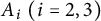 are saddles. Hence, the phase portraits on
$\Sigma _+^{\infty }$
 ,
$p(x_{1}=0)\cap R, \ p(x_{2}=0)\cap R$
 and
$ p(x_{3}=0)\cap R $
 are those in Table 5
$(11b)$
 .
Let
$\zeta _{13}$
 be the orbit of system (4.2) which originates from
$D_{13}$
 and tends toward
$D_{12}$
 . Then the intersection of the cone
$\overline {p\left (\mathcal {C}(\zeta _{13})\right )}$
 and
$\Sigma ^{\infty }_{+}$
 consists of
$p(V_{13})$
 ,
$p(V_{12})$
 and the orbit connecting
$p(V_{13})$
 and
$p(V_{12})$
 . Moreover, any orbit of the compactified vector field of system (1.3) on the cone
$p\left (\mathcal {C}(\zeta _{13})\right )$
 must originate from
$\overline {p(\Gamma _{13})}$
 and tend toward
$\overline {p(\Gamma _{12})}$
 , and any orbit of the compactified vector field of system (1.3) passing through a point in
$\mathring W^{u}(p(U_{13}))$
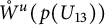 must be on the cone
$p\left (\mathcal {C}(\zeta _{13})\right )$
 and tend toward the attractor
$p(U_{12})$
 , because there are no other orbits of system (4.2) which emanate from
$D_{13}$
 in the interior of
$S_{3}$
 except
$\zeta _{13}$
 see Table 5
$(11a)$
 . The orbits of the compactified vector field of system (1.3) passing through a point in
$W^{u}(p(U_{23}))\bigcap \mathrm {Int}R$
 will tend toward the attractor
$p(U_{12})$
 , because all orbits of system (4.2) originating from
$D_{23}$
 in the interior of
$S_{3}$
 will tend toward
$D_{12}$
 see Table 5
$(11a)$
 .
Further verification shows that any orbit in the interior of the domain limited by
$p(x_{i}=0)~(i=1, 2, 3)$
 and
$W^{u}(p(B_{1}))\bigcup \bigcup \limits _{i=1}^{2} W^{u}(p(U_{i3}))$
 emanates from O and tends toward
$p(U_{12})$
 , and that any orbit in the interior of the domain limited by
$W^{u}(p(U_{23}))\bigcup p(\mathcal {C}(\zeta _{13}))$
 ,
$p(x_{i}=0)~(i=1, 2, 3)$
 and
$\Sigma ^{\infty }_{+}$
 emanates from
$p(V_{23})$
 and tends toward
$p(U_{12})$
 . Moreover, any orbit in the interior of the domain limited by
$p(x_{j}=0)~(j=2, 3)$
 ,
$\Sigma ^{\infty }_{+}$
 and
$W^{u}(p(B_{1}))\bigcup p(\mathcal {C}(\zeta _{13}))$
 emanates from
$p(A_{1})$
 and tends toward
$p(U_{12})$
 . This implies that the equilibrium
$p(U_{12})$
 is the global attractor in
$\mathrm {Int}R$
 . Hence, the global phase portrait in R is that in Table 5
$(11b)$
 .
Case 15. Referring to Tables 1 and 2, there exist the equilibria P and Q, which are saddles. Moreover,
$U_{12}$
 and
$U_{13}$
 are the attractors,
$A_{1}$
 and
$V_{23}$
 are repellers, and
$B_{3}$
 ,
$U_{23}$
 ,
$V_{12}$
 ,
$V_{13}$
 and
$A_{i}~(i=2, 3)$
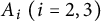 are saddles. Hence, the phase portraits on
$\Sigma _+^{\infty }$
 ,
$p(x_{1}=0)\cap R, \ p(x_{2}=0)\cap R$
 and
$ p(x_{3}=0)\cap R $
 are those in Table 5
$(12b)$
 .
For a given
$j\in \{2, 3\}$
 , let
$\zeta _{1j}$
 be the orbit of system (4.2) which originates from F and tends toward
$D_{1j}$
 . Then the intersection of the cone
$\overline {p\left (\mathcal {C}(\zeta _{1j})\right )}$
 and
$\Sigma ^{\infty }_{+}$
 consists of
$p(Q)$
 ,
$p(V_{1j})$
 and the orbit connecting
$p(Q)$
 and
$p(V_{1j})$
 . Moreover, any orbit of the compactified vector field of system (1.3) on the cone
$p\left (\mathcal {C}(\zeta _{1j})\right )$
 must originate from
$\overline {p(\Gamma )}$
 and tend toward
$\overline {p(\Gamma _{1j})}$
 . The two orbits of the compactified vector field of system (1.3) in
$\mathring W^{u}(p(P))$
 must be on the cones
$p\left (\mathcal {C}(\zeta _{12})\right )$
 and
$p\left (\mathcal {C}(\zeta _{13})\right )$
 respectively, in which one tends toward the attractor
$p(U_{12})$
 and the other tends toward the attractor
$p(U_{13})$
 , because there are no other orbits of system (4.2) which emanate from F in the interior of
$S_{3}$
 except
$\zeta _{12}$
 ,
$\zeta _{13}$
 and F see Table 5
$(12a)$
 . Let
$\xi _{23}$
 resp.
$\xi _{1}$
 be the orbit of system (4.2) which originates from
$D_{23}$
 resp.
$E_{1}$
 and tends toward F. Then the intersection of the cone
$\overline {p\left (\mathcal {C}(\xi _{23})\right )}$
 resp.
$\overline {p\left (\mathcal {C}(\xi _{1})\right )}$
 and
$\Sigma ^{\infty }_{+}$
 consists of
$p(V_{23})$
 resp.
$p(A_{1})$
 ,
$p(Q)$
 and the orbit connecting
$p(V_{23})$
 resp.
$p(A_{1})$
 and
$p(Q)$
 . Moreover, any orbit of the compactified vector field of system (1.3) on the cone
$p\left (\mathcal {C}(\xi _{23})\right )$
 resp.
$p\left (\mathcal {C}(\xi _{1})\right )$
 must originate from
$\overline {p(\Gamma _{23})}$
 resp. the
$x_{1}$
 -axis and tend toward
$\overline {p(\Gamma )}$
 . And the intersection of
$W^{u}(p(U_{23}))$
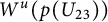 and
$p(\mathcal {C}(\xi _{23}))$
 consists of the orbit which emanates from
$p(U_{23})$
 and tends toward
$p(P)$
 . The intersection of
$W^{u}(p(B_{1}))$
 and
$p(\mathcal {C}(\xi _{1}))$
 consists of the orbit which emanates from
$p(B_{1})$
 and tends toward
$p(P)$
 .
For a given
$j\in \{2, 3\}$
 , any orbit in the interior of the domain limited by
$p(x_{i}=0)~(i\neq j)$
 ,
$\Sigma ^{\infty }_{+}$
 and
$p(\Gamma )\bigcup W^{u}(p(U_{23}))\bigcup p(\mathcal {C}(\zeta _{1j}))\bigcup p(\mathcal {C}(\xi _{23}))$
 emanates from
$p(V_{23})$
 and tends toward
$p(U_{1j})$
 . Moreover, any orbit in the interior of the domain limited by
$p(\Gamma )\bigcup W^{u}(p(B_{1}))\bigcup p(\mathcal {C}(\zeta _{1j}))\bigcup p(\mathcal {C}(\xi _{1}))$
 ,
$p(x_{i}=0)~(i\neq 1, j)$
 and
$\Sigma ^{\infty }_{+}$
 emanates from
$p(A_{1})$
 and tends toward
$p(U_{1j})$
 , and any orbit in the interior of the domain limited by
$p(x_{i}=0)~(i\neq j)$
 and
$p(\Gamma )\bigcup W^{u}(p(P))\bigcup W^{u}(p(B_{1})) \bigcup W^{u}(p(U_{23}))\bigcup p(\mathcal {C}(\xi _{23}))\bigcup p(\mathcal {C}(\xi _{1}))$
 emanates from O and tends toward
$p(U_{1j})$
 . Hence the global phase portrait in R is that in Table 5
$(12b)$
 .
Case 16. Because of
$J_{i}<0~(i=1, 2)$
 and
$J_{3}>0$
 , the equilibria P and Q do not exist. Moreover,
$B_{3}$
 is an attractor,
$A_{i}~(i=1, 2)$
 are repellers, and
$A_{3}$
 ,
$U_{12}$
 and
$V_{12}$
 are saddles. So the phase portraits on
$\Sigma _+^{\infty }$
 ,
$p(x_{1}=0)\cap R, \ p(x_{2}=0)\cap R$
 and
$ p(x_{3}=0)\cap R $
 are those in Table 5
$(13b)$
 .
Let
$\zeta _{12}$
 be the orbit of system (4.2) which originates from
$D_{12}$
 and tends toward
$E_{3}$
 . Moreover, the intersection of the cone
$\overline {p\left (\mathcal {C}(\zeta _{12})\right )}$
 and
$\Sigma ^{\infty }_{+}$
 consists of
$p(V_{12})$
 ,
$p(A_{3})$
 and the orbit connecting
$p(V_{12})$
 and
$p(A_{3})$
 . And any orbit of the compactified vector field of system (1.3) on the cone
$p\left (\mathcal {C}(\zeta _{12})\right )$
 must originate from
$\overline {p(\Gamma _{12})}$
 and tend toward the
$x_{3}$
 -axis. The orbit of the compactified vector field of system (1.3) passing through a point in
$\mathring W^{u}(p(U_{12}))$
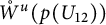 must be on the cone
$p\left (\mathcal {C}(\zeta _{12})\right )$
 and tend toward the attractor
$p(B_{3})$
 , because there are no other orbits of system (4.2) which emanate from
$D_{12}$
 in the interior of
$S_{3}$
 except
$\zeta _{12}$
 see Table 5
$(13a)$
 .
Some analysis shows that any orbit in the interior of the domain limited by
$p(x_{i}=0)~(i=1, 2, 3)$
 and
$\bigcup \limits _{k=1}^{2} W^{u}(p(B_{k}))\bigcup W^{u}(p(U_{12}))$
 emanates from O and tends toward
$p(B_{3})$
 , and that any orbit in the interior of the domain limited by
$W^{u}(p(B_{1}))\bigcup p(\mathcal {C}(\zeta _{12}))$
 ,
$p(x_{i}=0)~(i=2, 3)$
 and
$\Sigma ^{\infty }_{+}$
 emanates from
$p(A_{1})$
 and tends toward
$p(B_{3})$
 . Moreover, any orbit in the interior of the domain limited by
$p(x_{j}=0)~(j=1, 3)$
 ,
$\Sigma ^{\infty }_{+}$
 and
$W^{u}(p(B_{2}))\bigcup p(\mathcal {C}(\zeta _{12}))$
 emanates from
$p(A_{2})$
 and tends toward
$p(B_{3})$
 . This implies that the equilibrium
$p(B_{3})$
 is the global attractor in
$\mathrm {Int}R$
 . Hence, the global phase portrait in R is that in Table 5
$(13b)$
 .
Case 17. By Tables 1 and 2, the equilibria P and Q are saddles. And
$B_{3}$
 and
$U_{12}$
 are the attractors,
$A_{3}$
 and
$V_{12}$
 are saddles, and
$A_{i}~(i=1, 2)$
 are repellers. These show that the phase portraits on
$\Sigma _+^{\infty }$
 ,
$p(x_{1}=0)\cap R, \ p(x_{2}=0)\cap R$
 and
$ p(x_{3}=0)\cap R $
 are those in Table 5
$(14b)$
 .
For a given
$i\in \{1, 2\}$
 , let
$\zeta _{i}$
 be the orbit of system (4.2) which originates from
$E_{i}$
 and tends toward F. Then the intersection of the cone
$\overline {p\left (\mathcal {C}(\zeta _{i})\right )}$
 and
$\Sigma ^{\infty }_{+}$
 consists of
$p(A_{i})$
 ,
$p(Q)$
 and the orbit connecting
$p(A_{i})$
 and
$p(Q)$
 . Moreover, any orbit of the compactified vector field of system (1.3) on the cone
$p\left (\mathcal {C}(\zeta _{i})\right )$
 must originate from the
$x_{i}$
 -axis and tend toward
$\overline {p(\Gamma )}$
 . And the intersection of
$W^{u}(p(B_{i}))$
 and
$p(\mathcal {C}(\zeta _{i}))$
 consists of the orbit which emanates from
$p(B_{i})$
 and tends toward
$p(P)$
 . Let
$\xi _{12}$
 resp.
$\xi _{3}$
 be the orbit of system (4.2) which originates from F and tends toward
$D_{12}$
 resp.
$E_{3}$
 . Then the intersection of the cone
$\overline {p\left (\mathcal {C}(\xi _{12})\right )}$
 resp.
$\overline {p\left (\mathcal {C}(\xi _{3})\right )}$
 and
$\Sigma ^{\infty }_{+}$
 consists of
$p(Q)$
 ,
$p(V_{12})$
 resp.
$p(A_{3})$
 and the orbit connecting the equilibrium
$p(Q)$
 and the equilibrium
$p(V_{12})$
 resp.
$p(A_{3})$
 . From (4.1) it follows that any orbit of the compactified vector field of system (1.3) on the cone
$p\left (\mathcal {C}(\xi _{12})\right )$
 resp.
$p\left (\mathcal {C}(\xi _{3})\right )$
 must originate from
$\overline {p(\Gamma )}$
 and tend toward
$\overline {p(\Gamma _{12})}$
 resp. the
$x_{3}$
 -axis. The two orbits of the compactified vector field of system (1.3) in
$\mathring W^{u}(p(P))$
 must be on the cones
$p\left (\mathcal {C}(\xi _{12})\right )$
 and
$p\left (\mathcal {C}(\xi _{3})\right )$
 respectively, in which one tends toward the attractor
$p(U_{12})$
 and the other tends toward the attractor
$p(B_{3})$
 , because there are no other orbits of the system (4.2) which emanate from F in the interior of
$S_{3}$
 except
$\xi _{12}$
 ,
$\xi _{3}$
 and F see Table 5
$(14a)$
 .
Further verification shows that any orbit in the interior of the domain limited by
$p(x_{i}=0)~(i=1, 2)$
 and
$p(\Gamma )\bigcup W^{u}(p(P))\bigcup \bigcup \limits _{k=1}^{2}\big (W^{u}(p(B_{k}))\bigcup p(\mathcal {C}(\zeta _{k}))\big )$
 emanates from O and tends toward
$p(B_{3})$
 , and that any orbit in the interior of the domain limited by
$p(x_{3}=0)$
 and
$p(\Gamma )\bigcup W^{u}(p(P))\bigcup \bigcup \limits _{k=1}^{2}\big (W^{u}(p(B_{k}))\bigcup p(\mathcal {C}(\zeta _{k}))\big )$
 emanates from O and tends toward
$p(U_{12})$
 . Moreover, one can check that for a given
$i\in \{1, 2\}$
 , all orbits in the interior of the domain limited by
$p(x_{3}=0)$
 ,
$\Sigma ^{\infty }_{+}$
 and
$p(\Gamma )\bigcup W^{u}(p(B_{i}))\bigcup p(\mathcal {C}(\zeta _{i}))\bigcup p(\mathcal {C}(\xi _{12}))$
 emanate from
$p(A_{i})$
 and tend toward
$p(U_{12})$
 , and that any orbit in the interior of the domain limited by
$ p(\Gamma )\bigcup W^{u}(p(B_{i}))\bigcup p(\mathcal {C}(\zeta _{i}))\bigcup p(\mathcal {C}(\xi _{3}))$
 ,
$p(x_{j}=0)~(j\neq i, 3)$
 and
$\Sigma ^{\infty }_{+}$
 emanates from
$p(A_{i})$
 and tends toward
$p(B_{3})$
 . So the global phase portrait in R is that in Table 5
$(14b)$
 .
Case 18. Because
$J_{i}~(i=1, 2, 3)$
 have different signs, it follows from Tables 1 and 2 that the equilibria P and Q do not exist, and that
$U_{12}$
 is an attractor,
$A_{3}$
 is a repeller, and
$B_{3}$
 ,
$V_{12}$
 and
$A_{i}~(i=1, 2)$
 are saddles. Hence the phase portraits on
$\Sigma _+^{\infty }$
 ,
$p(x_{1}=0)\cap R, \ p(x_{2}=0)\cap R$
 and
$ p(x_{3}=0)\cap R$
 are those in Table 5
$(15b)$
 . Furthermore, any orbit in the interior of the domain limited by
$p(x_{i}=0)~(i=1, 2, 3)$
 and
$W^{u}(p(B_{3}))$
 emanates from O and tends toward
$p(U_{12})$
 , and any orbit in the interior of the domain limited by
$W^{u}(p(B_{3}))$
 ,
$p(x_{i}=0)~(i=1, 2, 3)$
 and
$\Sigma ^{\infty }_{+}$
 emanates from
$p(A_{3})$
 and tends toward
$p(U_{12})$
 . Hence, the equilibrium
$p(U_{12})$
 attracts all points in
$\mathrm {Int}R$
 , and so the global phase portrait in R is that in Table 5
$(15b)$
 .
Case 21. It follows from
$J_{i}>0~(i=1, 2, 3)$
 and
$\Phi <0$
 that the positive finite equilibrium P and the positive equilibrium at infinity Q both exist. The former is an attractor and the latter is a saddle, whose stable manifold is located in the positive plane at infinity and unstable manifold lies on the ray
$\Gamma $
 in between P and Q. By Tables 1 and 2, it follows that
$B_{3}$
 ,
$U_{12}$
 ,
$U_{13}$
 ,
$U_{23}$
 ,
$V_{12}$
 ,
$V_{13}$
 , and
$V_{23}$
 are saddles, and
$A_{i}~(i=1, 2, 3)$
 are repellers. Hence, the phase portraits on
$\Sigma _+^{\infty }$
 ,
$p(x_{1}=0)\cap R, \ p(x_{2}=0)\cap R$
 and
$ p(x_{3}=0)\cap R $
 are those in Table 5
$(16b)$
 .
For any given two integers
$i,\ j~(1\leq i<j\leq 3)$
 , we assume that
$\zeta _{ij}$
 is the orbit of system (4.2) which emanates from the saddle
$D_{ij}$
 and tends toward the attractor F. Then the intersection of the cone
$\overline {p\left (\mathcal {C}(\zeta _{ij})\right )}$
 and
$\Sigma ^{\infty }_{+}$
 consists of
$p(V_{ij})$
 ,
$p(Q)$
 and the orbit connecting
$p(V_{ij})$
 and
$p(Q)$
 . Moreover, any orbit of the compactified vector field of system (1.3) on the cone
$p\left (\mathcal {C}(\zeta _{ij})\right )$
 must originate
$\overline {p(\Gamma _{ij})}$
 and tend toward
$\overline {p(\Gamma )}$
 . Any orbit of the compactified vector field of system (1.3) passing through a point in
$ \mathring W^{u}(p(U_{ij}))$
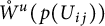 must be on the cone
$p\left (\mathcal {C}(\zeta _{ij})\right )$
 and tend toward the attractor
$p(P)$
 , because there are no other orbits of system (4.2) which emanate from
$D_{ij}$
 in the interior of
$S_{3}$
 except
$\zeta _{ij}$
 see Table 5
$(16a)$
 .
One can check that all the orbits in the interior of the domain limited by the invariant surface
$p(P)\bigcup \bigcup \limits _{k=1}^{3}W^{u}(p(B_{k}))\bigcup \bigcup \limits _{1\leq i<j\leq 3}W^{u}(p(U_{ij}))$
 and
$p(x_{i}=0)~( i=1, 2, 3)$
 emanate from O and tend toward
$p(P)$
 . For
$i\in \{1, 2, 3\}$
 , each orbit in the interior of the domain limited by
$p(\Gamma )\bigcup W^{u}(p(B_{i}))\bigcup \bigcup \limits _{j>i}p(\mathcal {C}(\zeta _{ij}))\bigcup \bigcup \limits _{j<i}p(\mathcal {C}(\zeta _{ji}))$
 ,
$p(x_{j}=0)~(j\neq i)$
 and
$\Sigma ^{\infty }_{+}$
 emanates from
$p(A_{i})$
 and tends toward
$p(P)$
 . This implies that the equilibrium
$p(P)$
 is the global attractor in
$\mathrm {Int}R$
 . Hence, the global phase portrait in R is that in Table 5
$(16b)$
 .
Case 22. Owing to
$J_{i}>0~(i=1, 2)$
 and
$J_{3}<0 $
 , the equilibria P and Q do not exist. Referring to Tables 1 and 2,
$U_{12}$
 is an attractor,
$A_{i}~(i=1, 2, 3)$
 are repellers, and
$B_{3}$
 ,
$U_{13}$
 ,
$U_{23}$
 ,
$V_{12}$
 ,
$V_{13}$
 and
$V_{23}$
 are saddles. Hence, the phase portraits on
$\Sigma _+^{\infty }$
 ,
$p(x_{1}=0)\cap R, \ p(x_{2}=0)\cap R$
 and
$ p(x_{3}=0)\cap R $
 are those in Table 5
$(17b)$
 .
For a given
$i\in \{1, 2\}$
 , let
$\zeta _{i3}$
 be the orbit of system (4.2) which originates from
$D_{i3}$
 and tends toward
$D_{12}$
 . Then the intersection of the cone
$\overline {p\left (\mathcal {C}(\zeta _{i3})\right )}$
 and
$\Sigma ^{\infty }_{+}$
 consists of
$p(V_{i3})$
 ,
$p(V_{12})$
 and the orbit connecting
$p(V_{i3})$
 and
$p(V_{12})$
 . Moreover, any orbit of the compactified vector field of system (1.3) on the cone
$p\left (\mathcal {C}(\zeta _{i3})\right )$
 must originate from
$\overline {p(\Gamma _{i3})}$
 and tend toward
$\overline {p(\Gamma _{12})}$
 . And any orbit of the compactified vector field of system (1.3) passing through a point in
$\mathring W^{u}(p(U_{i3}))$
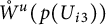 must be on the cone
$p\left (\mathcal {C}(\zeta _{i3})\right )$
 and tend toward the attractor
$p(U_{12})$
 , because there are no other orbits of system (4.2) which emanate from
$D_{i3}$
 in the interior of
$S_{3}$
 except
$\zeta _{i3}$
 see Table 5
$(17a)$
 . Moreover, any orbit in the interior of the domain limited by
$p(x_{i}=0)~(i=1, 2, 3)$
 and
$\bigcup \limits _{k=1}^{3}W^{u}(p(B_{k}))\bigcup \bigcup \limits _{i=1}^{2}W^{u}(p(U_{i3}))$
 emanates from O and tends toward
$p(U_{12})$
 . For a given
$i\in \{1, 2\}$
 , each orbit in the interior of the domain limited by
$p(x_{j}=0)~(j\neq i)$
 ,
$\Sigma ^{\infty }_{+}$
 and
$W^{u}(p(B_{i}))\bigcup p(\mathcal {C}(\zeta _{i3}))$
 emanates from
$p(A_{i})$
 and tends toward
$p(U_{12})$
 . Furthermore, any orbit in the interior of the domain limited by
$p(x_{j}=0)~(j=1, 2)$
 ,
$\Sigma ^{\infty }_{+}$
 and
$p(\Gamma _{12})\bigcup W^{u}(p(B_{3}))\bigcup \bigcup \limits _{i=1}^{2}p(\mathcal {C}(\zeta _{i3}))$
 emanates from
$p(A_{3})$
 and tends toward
$p(U_{12})$
 . This implies that the equilibrium
$p(U_{12})$
 is the global attractor in
$\mathrm {Int}R$
 . So the global phase portrait in R is that in Table 5
$(17b)$
 .
Case 32. Owing to
$J_{1}>0$
 and
$J_{3}<0$
 , the equilibria P and Q do not exist. Referring to Tables 1 and 2,
$V_{12}$
 is an attractor,
$A_{1}$
 is a repeller, and
$A_{i}~(i=2, 3)$
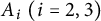 and
$B_{3}$
 are saddles. From Proposition 3.3,
$\Gamma _{12}$
 is a characteristic line of
$V_{12}$
 corresponding to the eigenvalue
$\frac {I_{12}} {\alpha _1}$
 . By the Poincaré–Bendixson theorem and the invariance of the considered planes, we can obtain the global phase portraits on
$\Sigma _+^{\infty }$
 ,
$p(x_{1}=0)\cap R, \ p(x_{2}=0)\cap R$
 and
$ p(x_{3}=0)\cap R $
 , which are described in Table 5
$(18b)$
 .
Further analysis shows that any orbit in the interior of the domain limited by
$p(x_{i}=0)~(i=1, 2, 3)$
 and
$p(V_{12})\bigcup W^{u}(p(B_{1}))$
 emanates from O and tends toward
$p(V_{12})$
 , and that any orbit in the interior of the domain limited by
$p(x_{j}=0)~(j=1, 2, 3)$
 ,
$\Sigma ^{\infty }_{+}$
 and
$W^{u}(p(B_{1}))$
 emanates from
$p(A_{1})$
 and tends toward
$p(V_{12})$
 . Moreover, the equilibrium
$p(V_{12})$
 is a global attractor in
$\mathrm { Int}R$
 . So the global phase portrait in R is that in Table 5
$(18b)$
 .
Case 33. Because of
$J_{1}>0$
 and
$J_{3}<0$
 , the equilibria P and Q do not exist. Referring to Tables 1 and 2,
$B_{3}$
 and
$V_{12} $
 are the attractors,
$A_{1}$
 is a repeller, and
$A_{i}~(i=2, 3)$
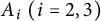 ,
$U_{23}$
 and
$V_{23}$
 are saddles. From Proposition 3.3,
$\Gamma _{12}$
 is a characteristic line of
$V_{12}$
 corresponding to the eigenvalue
$\frac {I_{12}} {\alpha _1}$
 . These show that the phase portraits on
$\Sigma _+^{\infty }$
 ,
$p(x_{1}=0)\cap R, \ p(x_{2}=0)\cap R$
 and
$ p(x_{3}=0)\cap R $
 are those in Table 5
$(19b)$
 .
Let
$\zeta _{23}$
 be the orbit of system (4.2) which emanates from
$E_{1}$
 and tends toward
$D_{23}$
 . Then the intersection of
$\overline {p\left (\mathcal {C}(\zeta _{23})\right )}$
 and
$\Sigma ^{\infty }_{+}$
 consists of
$p(A_{1})$
 ,
$p(V_{23})$
 and the orbit connecting the equilibrium
$p(A_{1})$
 and the equilibrium
$p(V_{23})$
 . Moreover, any orbit of the compactified vector field of system (1.3) on the cone
$p\left (\mathcal {C}(\zeta _{23})\right )$
 must originate from the
$x_{1}$
 -axis and tend toward
$\overline {p(\Gamma _{23})}$
 . The two-dimensional stable manifold of
$p((U_{23}))$
 must be the cone
$\overline {p\left (\mathcal {C}(\zeta _{23})\right )}$
 , because there are no other orbits of system (4.2) which tend toward
$D_{23}$
 in the interior of
$S_{3}$
 except
$\zeta _{23}$
 see Table 5
$(19a)$
 .
Some analysis shows that any orbit in the interior of the domain limited by
$p(x_{i}=0)~(i=1, 3)$
 and
$p(V_{12})\bigcup W^{u}(p(B_{1})) \bigcup p(\mathcal {C}(\zeta _{23}))$
 emanates from O and tends toward
$p(V_{12})$
 , and that any orbit in the interior of the domain limited by
$p(x_{j}=0)~(j=1, 2)$
 and
$W^{u}(p(B_{1}))\bigcup p(\mathcal {C}(\zeta _{23}))$
 emanates from O and tends toward
$p(B_{3})$
 . Moreover, any orbit in the interior of the domain limited by
$p(x_{j}=0)~(j=1, 3)$
 ,
$\Sigma ^{\infty }_{+}$
 and
$ W^{u}(p(B_{1}))\bigcup p(\mathcal {C}(\zeta _{23}))$
 emanates from
$p(A_{1})$
 and tends toward
$p(V_{12})$
 . And any orbit in the interior of the domain limited by
$p(x_{j}=0)~(j=1, 2)$
 ,
$\Sigma ^{\infty }_{+}$
 and
$ W^{u}(p(B_{1}))\bigcup p(\mathcal {C}(\zeta _{23}))$
 emanates from
$p(A_{1})$
 and tends toward
$p(B_{3})$
 . So the global phase portrait in R is that in Table 5
$(19b)$
 .
Case 34. By Tables 1 and 2, it follows that the equilibria P and Q exist and are saddles, and that
$B_{3}$
 and
$V_{12}$
 are the attractors,
$A_{1}$
 and
$V_{23}$
 are repellers, and
$A_{i}~(i=2, 3)$
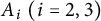 and
$U_{23}$
 are saddles. From Proposition 3.3,
$\Gamma _{12}$
 is a characteristic line of
$V_{12}$
 corresponding to the eigenvalue
$\frac {I_{12}} {\alpha _1}$
 . So the phase portraits on
$\Sigma _+^{\infty }$
 ,
$p(x_{1}=0)\cap R, \ p(x_{2}=0)\cap R$
 , and
$ p(x_{3}=0)\cap R $
 are those in Table 5
$(20b)$
 .
Let
$\zeta _{12}$
 resp.
$\zeta _{3}$
 be the orbit of system (4.2) which originates from F and tends toward
$D_{12}$
 resp.
$E_{3}$
 . Then the intersection of the cone
$\overline {p\left (\mathcal {C}(\zeta _{12})\right )}$
 resp.
$\overline {p\left (\mathcal {C}(\zeta _{3})\right )}$
 and
$\Sigma ^{\infty }_{+}$
 consists of
$p(Q)$
 ,
$p(V_{12})$
 resp.
$p(A_{3})$
 and the orbit connecting the equilibrium
$p(Q)$
 and the equilibrium
$p(V_{12})$
 resp.
$p(A_{3})$
 . Moreover, any orbit of the compactified vector field of system (1.3) on the cone
$p\left (\mathcal {C}(\zeta _{12})\right )$
 resp.
$p\left (\mathcal {C}(\zeta _{3})\right )$
 must originate from
$\overline {p(\Gamma )}$
 and tend toward
$\overline {p(\Gamma _{12})}$
 (resp. the
$x_{3}$
 -axis). The two orbits of the compactified vector field of system (1.3) in
$\mathring W^{u}(p(P))$
 must be on the cones
$p\left (\mathcal {C}(\zeta _{12})\right )$
 and
$p\left (\mathcal {C}(\zeta _{3})\right )$
 , respectively, in which one tends toward the attractor
$p(V_{12})$
 and the other tends toward the attractor
$p(B_{3})$
 , because there are no other orbits of system (4.2) which emanate from F in the interior of
$S_{3}$
 except
$\zeta _{12}$
 ,
$\zeta _{3}$
 , and F see Table 5
$(20a)$
 . Let
$\xi _{23}$
 resp.
$\xi _{1}$
 be the orbit of system (4.2) which originates from
$D_{23}$
 resp.
$E_{1}$
 and tends toward F. Then the intersection of the cone
$\overline {p\left (\mathcal {C}(\xi _{23})\right )}$
 resp.
$\overline {p\left (\mathcal {C}(\xi _{1})\right )}$
 and
$\Sigma ^{\infty }_{+}$
 consists of
$p(V_{23})$
 resp.
$p(A_{1})$
 ,
$p(Q)$
 and the orbit connecting
$p(V_{23})$
 resp.
$p(A_{1})$
 and
$p(Q)$
 . Moreover, any orbit of the compactified vector field of system (1.3) on the cone
$p\left (\mathcal {C}(\xi _{23})\right )$
 resp.
$p\left (\mathcal {C}(\xi _{1})\right )$
 must originate from
$\overline {p(\Gamma _{23})}$
 resp. the
$x_{1}$
 -axis and tend toward
$\overline {p(\Gamma )}$
 . And the intersection of
$W^{u}(p(U_{23}))$
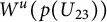 and
$p(\mathcal {C}(\xi _{23}))$
 consists of the orbit which emanates from
$p(U_{23})$
 and tends toward
$p(P)$
 .
$W^{u}(p(B_{1}))$
 and
$p(\mathcal {C}(\xi _{1})) $
 must insect at one orbit which emanates from
$p(B_{1})$
 and tends toward
$p(P)$
 .
Further verification shows that any orbit in the interior of the domain limited by
$p(x_{3}=0)$
 ,
$\Sigma ^{\infty }_{+}$
 and
$p(\Gamma )\bigcup W^{u}(p(B_{1}))\bigcup p(\mathcal {C}(\zeta _{12}))\bigcup p(\mathcal {C}(\xi _{1}))$
 emanates from
$p(A_{1})$
 and tends toward
$p(V_{12})$
 , and that any orbit in the interior of the domain limited by
$p(x_{2}=0)$
 ,
$\Sigma ^{\infty }_{+}$
 and
$p(\Gamma )\bigcup W^{u}(p(B_{1}))\bigcup p(\mathcal {C}(\zeta _{3}))\bigcup p(\mathcal {C}(\xi _{1}))$
 emanates from
$p(A_{1})$
 and tends toward
$p(B_{3})$
 . Moreover, one can check that any orbit in the interior of the domain limited by
$ p(\Gamma )\bigcup W^{u}(p(U_{23}))\bigcup p(\mathcal {C}(\zeta _{12}))\bigcup p(\mathcal {C}(\xi _{23}))$
 ,
$p(x_{j}=0)~(j=1, 3)$
 and
$\Sigma ^{\infty }_{+}$
 emanates from
$p(V_{23})$
 and tends toward
$p(V_{12})$
 , and that the orbits in the interior of the domain limited by
$p(x_{1}=0)$
 ,
$\Sigma ^{\infty }_{+}$
 and
$ W^{u}(p(U_{23}))\bigcup p(\mathcal {C}(\zeta _{3}))\bigcup p(\mathcal {C}(\xi _{23}))\bigcup p(\Gamma )$
 move away from
$p(V_{23})$
 and tend toward
$p(B_{3})$
 . The orbits in the interior of the domain limited by
$p(x_{j}=0)~(j=1, 2)$
 and
$ W^{u}(p(P))\bigcup W^{u}(p(B_{1}))\bigcup W^{u}(p(U_{23}))\bigcup p(\mathcal {C}(\xi _{23}))\bigcup p(\mathcal {C}(\xi _{1}))\bigcup p(\Gamma )$
 emanate from O and tend toward
$p(B_{3})$
 . The orbits in the interior of the domain limited by
$p(\Gamma )\bigcup W^{u}(p(P))\bigcup W^{u}(p(B_{1})) \bigcup W^{u}(p(U_{23}))\bigcup p(\mathcal {C}(\xi _{23}))\bigcup p(\mathcal {C}(\xi _{1}))$
 and
$p(x_{j}=0)~(j=1, 3)$
 emanate from O and tend toward
$p(V_{12})$
 . So the global phase portrait in R is that in Table 5
$(20b)$
 .
Case 35. Owing to
$J_{1}>0$
 and
$J_{i}<0~(i=2, 3)$
 , the equilibria P and Q do not exist. Referring to Tables 1 and 2,
$V_{12}$
 is an attractor,
$V_{13}$
 is a repeller, and
$B_{3} $
 ,
$U_{13}$
 and
$A_{i}~(i=1, 2, 3)$
 are saddles. From Proposition 3.3,
$\Gamma _{12}$
 is a characteristic line of
$V_{12}$
 corresponding to the eigenvalue
$\frac {I_{12}} {\alpha _1}$
 . Hence, the phase portraits on
$\Sigma _+^{\infty }$
 ,
$p(x_{1}=0)\cap R, \ p(x_{2}=0)\cap R$
 and
$ p(x_{3}=0)\cap R $
 are those in Table 5
$(21b)$
 .
For the compactified vector field of system (1.3), any orbit passing through a point in
$W^{u}(p(U_{13}))\bigcap \mathrm {Int}R$
 will tend toward the attractor
$p(V_{12})$
 , because all orbits which originate from
$D_{13}$
 in the interior of
$S_{3}$
 will tend toward
$D_{12}$
 see Table 5
$(21a)$
 . Any orbit in the interior of the domain limited by
$p(x_{j}=0)~(j=1, 2, 3)$
 and
$p(V_{12})\bigcup W^{u}(p(U_{13}))$
 emanates from O and tends toward
$p(V_{12})$
 . Any orbit in the interior of the domain limited by
$p(x_{i}=0)~(i=1, 2, 3)$
 ,
$\Sigma ^{\infty }_{+}$
 and
$ W^{u}(p(U_{13}))$
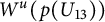 emanates from
$p(V_{13})$
 and tends toward
$p(V_{12})$
 . The equilibrium
$p(V_{12})$
 attracts all points in
$\mathrm {Int}R$
 . Hence, the global phase portrait in R is that in Table 5
$(21b)$
 .
Case 36. Owing to
$J_{2}>0$
 and
$J_{3}<0 $
 , the equilibria P and Q do not exist. By Tables 1 and 2,
$V_{12}$
 is an attractor,
$A_{i}~(i=1, 3)$
 are repellers, and
$B_{3}$
 ,
$A_{2}$
 ,
$U_{13}$
 , and
$V_{13}$
 are saddles. From Proposition 3.3,
$\Gamma _{12}$
 is a characteristic line of
$V_{12}$
 corresponding to the eigenvalue
$\frac {I_{12}} {\alpha _1}$
 . Hence, the phase portraits on
$\Sigma _+^{\infty }$
 ,
$p(x_{1}=0)\cap R, \ p(x_{2}=0)\cap R$
 and
$ p(x_{3}=0)\cap R $
 are those in Table 5
$(22b)$
 .
Let
$\zeta _{13}$
 be the orbit of system (4.2) which emanates from
$D_{13}$
 and tends toward
$D_{12}$
 . The invariance of the cone
$p\left (\mathcal {C}(\zeta _{13})\right )$
 causes the intersection of
$\overline {p\left (\mathcal {C}(\zeta _{13})\right )}$
 and
$\Sigma ^{\infty }_{+}$
 consists of
$p(V_{13})$
 ,
$p(V_{12})$
 and the orbit connecting
$p(V_{13})$
 and
$p(V_{12})$
 . By (4.1) it follows that any orbit of the compactified vector field of system (1.3) on the cone
$p\left (\mathcal {C}(\zeta _{13})\right )$
 must originate from
$\overline {p(\Gamma _{13})}$
 and tend toward
$\overline {p(\Gamma _{12})}$
 , and that any orbit of the compactified vector field of system (1.3) passing through a point in
$\mathring W^{u}(p(U_{13}))$
 must be on the cone
$p\left (\mathcal {C}(\zeta _{13})\right )$
 and tend toward the attractor
$p(V_{12})$
 , because there are no other orbits of the system (4.2) emanating from
$D_{13}$
 in the interior of
$S_{3}$
 except
$\zeta _{13}$
 see Table 5
$(22a)$
 .
Further analysis shows that any orbit in the interior of the domain limited by
$p(x_{i}=0)~(i=1, 2, 3)$
 and
$p(V_{12})\bigcup W^{u}(p(B_{1}))\bigcup W^{u}(p(B_{3}))\bigcup W^{u}(p(U_{13}))$
 emanates from O and tends toward
$p(V_{12})$
 . Any orbit in the interior of the domain limited by
$p(x_{j}=0)~(j=1, 2, 3)$
 ,
$\Sigma ^{\infty }_{+}$
 and
$W^{u}(p(B_{3}))\bigcup p(\mathcal {C}(\zeta _{13}))$
 emanates from
$p(A_{3})$
 and tends toward
$p(V_{12})$
 . Any orbit in the interior of the domain limited by
$p(x_{j}=0)~(j=2, 3)$
 ,
$\Sigma ^{\infty }_{+}$
 and
$W^{u}(p(B_{1}))\bigcup p(\mathcal {C}(\zeta _{13}))$
 emanates from
$p(A_{1})$
 and tends toward
$p(V_{12})$
 . The equilibrium
$p(V_{12})$
 attracts all points in
$\mathrm {Int}R$
 . So, the global phase portraits in R are described in Table 5
$(22b)$
 .
Case 37. It follows from
$J_{i}>0~(i=1, 2, 3)$
 and
$\Phi <0$
 that the positive finite equilibrium P and the positive equilibrium at infinity Q both exist. The former is an attractor and the latter is a saddle, whose stable manifold is located in the positive plane at infinity and the unstable manifold lies on the ray
$\Gamma $
 in between P and Q. By Tables 1 and 2,
$A_{i}~(i=1, 2)$
 are repellers, and
$B_{3}$
 ,
$A_{3}$
 ,
$U_{23}$
 ,
$V_{12}$
 and
$V_{23}$
 are saddles. From Proposition 3.3,
$\Gamma _{12}$
 is a characteristic line of
$V_{12}$
 corresponding to the eigenvalue
$\frac {I_{12}}{\alpha _1}$
 . So the phase portraits on
$\Sigma _+^{\infty }$
 ,
$p(x_{1}=0)\cap R, \ p(x_{2}=0)\cap R$
 and
$ p(x_{3}=0)\cap R $
 are those in Table 5
$(23b)$
 .
Let
$\zeta _{23}$
 be the orbit of system (4.2) which originates from
$D_{23}$
 and tends toward F. The invariance of the cone
$p\left (\mathcal {C}(\zeta _{23})\right )$
 causes that the intersection of the cone
$\overline {p\left (\mathcal {C}(\zeta _{23})\right )}$
 and
$\Sigma ^{\infty }_{+}$
 consists of intersect on
$p(V_{23})$
 ,
$p(Q)$
 and the orbit connecting
$p(V_{23})$
 and
$p(Q)$
 . Moreover, for the compactified vector field of system (1.3) any orbit on the cone
$p\left (\mathcal {C}(\zeta _{23})\right )$
 must originate from
$\overline {p(\Gamma _{23})}$
 and tend toward
$\overline {p(\Gamma )}$
 . Any orbit passing through a point in
$\mathring W^{u}(p(U_{23}))$
 must be on the cone
$p\left (\mathcal {C}(\zeta _{23})\right )$
 and tend toward the attractor
$p(P)$
 , because there is no an orbits of system (4.2) which emanate from
$D_{23}$
 in the interior of
$S_{3}$
 except
$\zeta _{23}$
 see Table 5
$(23a)$
 .
Furthermore, any orbit in the interior of the domain limited by
$p(x_{i}=0)~(i=1, 2, 3)$
 ,
$\Sigma ^{\infty }_{+}$
 and
$p(P)\bigcup W^{u}(p(Q))\bigcup W^{u}(p(V_{12}))\bigcup W^{u}(p(B_{1}))\bigcup p(\mathcal {C}(\zeta _{23}))$
 emanates from
$p(A_{1})$
 and tends toward
$p(P)$
 . Any orbit in the interior of the domain limited by
$p(P)\bigcup \bigcup \limits _{k=1}^{2}W^{u}(p(B_{k}))\bigcup W^{u}(p(U_{23}))\bigcup W^{u}(p(V_{12}))\bigcup W^{u}(p(Q))$
 and
$p(x_{i}=0)~(i=1, 2, 3)$
 tends away from O and tends toward
$p(P)$
 . Any orbit in the interior of the domain limited by
$p(x_{j}=0)~(j=1, 3)$
 ,
$\Sigma ^{\infty }_{+}$
 and
$p(P)\bigcup W^{u}(p(Q)) \bigcup W^{u}(p(V_{12}))\bigcup W^{u}(p(B_{2}))\bigcup p(\mathcal {C}(\zeta _{23}))$
 emanates from
$p(A_{2})$
 and tends toward
$p(P)$
 . These together with the fact that the equilibrium
$p(P)$
 is the global attractor in
$\mathrm {Int}R$
 show that the global phase portrait in R is that in Table 5
$(23b)$
 .
Case 38. Owing to
$J_{1}<0$
 and
$J_{3}>0 $
 , the equilibria P and Q do not exist. Referring to Tables 1 and 2,
$U_{23}$
 is an attractor,
$A_{i}~(i=1, 2)$
 are repellers, and
$B_{3}$
 ,
$A_{3}$
 ,
$V_{12}$
 , and
$V_{23}$
 are saddles. From Proposition 3.3,
$\Gamma _{12}$
 is a characteristic line of
$V_{12}$
 corresponding to the eigenvalue
$\frac {I_{12}} {\alpha _1}$
 . So the phase portraits on
$\Sigma _+^{\infty }$
 ,
$p(x_{1}=0)\cap R, \ p(x_{2}=0)\cap R$
 and
$ p(x_{3}=0)\cap R $
 are those in Table 5
$(24b)$
 .
Some analysis shows that any orbit in the interior of the domain limited by
$p(x_{i}=0)~(i=1, 2, 3)$
 and
$\bigcup \limits _{k=1}^{2}\big (W^{u}(p(B_{k}))\bigcup W^{u}(p(V_{k,k+1})\big )$
 tends away from O and tends toward
$p(U_{23})$
 . Any orbit in the interior of the domain limited by
$p(x_{i}=0)~(i=1, 2, 3)$
 ,
$\Sigma ^{\infty }_{+}$
 and
$W^{u}(p(B_{1}))\bigcup \bigcup \limits _{i=1}^{2}W^{u}(p(V_{i,i+1}))$
 emanates from
$p(A_{1})$
 and tends toward
$p(U_{23})$
 . And the orbits in the interior of the domain limited by
$p(x_{j}=0)~(j=1, 3)$
 ,
$\Sigma ^{\infty }_{+}$
 and
$W^{u}(p(B_{2}))\bigcup \bigcup \limits _{i=1}^{2}W^{u}(p(V_{i,i+1}))$
 emanates from
$p(A_{2})$
 and tends toward
$p(U_{23})$
 . Moreover, the equilibrium
$p(U_{23})$
 attracts all points in
$\mathrm {Int}R$
 . Hence, the global phase portrait in R is that in Table 5
$(24b)$
 .
Case 39. Because of
$J_{1}>0$
 and
$J_{3}<0$
 , the equilibria P and Q do not exist. Referring to Tables 1 and 2,
$V_{12}$
 is an attractor,
$A_{i}~(i=1, 2)$
 are repellers, and
$B_{3}$
 ,
$A_{3}$
 ,
$U_{23}$
 , and
$V_{23}$
 are saddles. From Proposition 3.3,
$\Gamma _{12}$
 is a characteristic line of
$V_{12}$
 corresponding to the eigenvalue
$\frac {I_{12}} {\alpha _1}$
 . So the phase portraits on
$\Sigma _+^{\infty }$
 ,
$p(x_{1}=0)\cap R, \ p(x_{2}=0)\cap R$
 and
$ p(x_{3}=0)\cap R $
 are those in Table 5
$(25b)$
 .
Let
$\zeta _{23}$
 be the orbit of system (4.2) which originates from
$D_{23}$
 and tends toward
$D_{12}$
 . Then the intersection of the cone
$\overline {p\left (\mathcal {C}(\zeta _{23})\right )}$
 and
$\Sigma ^{\infty }_{+}$
 consists of
$p(V_{23})$
 ,
$p(V_{12})$
 and the orbit connecting
$p(V_{23})$
 and
$p(V_{12})$
 . Moreover, for the compactified vector field of system (1.3) any orbit on the cone
$p\left (\mathcal {C}(\zeta _{23})\right )$
 must originate from
$\overline {p(\Gamma _{23})}$
 and tend toward
$\overline {p(\Gamma _{12})}$
 . Any orbit passing through a point in
$\mathring W^{u}(p(U_{23}))$
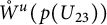 must be on the cone
$p\left (\mathcal {C}(\zeta _{23})\right )$
 and tend toward the attractor
$p(V_{12})$
 , because there are no other orbits of system (4.2) which emanate from
$D_{23}$
 in the interior of
$S_{3}$
 except
$\zeta _{23}$
 see Table 5
$(25a)$
 .
Further verification shows that any orbit in the interior of the domain limited by
$p(x_{i}=0)~(i=1, 2, 3)$
 and
$p(V_{12})\bigcup \bigcup \limits _{k=1}^{2}W^{u}(p(B_{k}))\bigcup W^{u}(p(U_{23}))$
 emanates from O and tends toward
$p(V_{12})$
 . Any orbit in the interior of the domain limited by
$p(x_{i}=0)~(i=1, 2, 3)$
 ,
$\Sigma ^{\infty }_{+}$
 and
$W^{u}(p(B_{1}))\bigcup p(\mathcal {C}(\zeta _{23}))$
 emanates from
$p(A_{1})$
 and tends toward
$p(V_{12})$
 . Any orbit in the interior of the domain limited by
$p(x_{j}=0)~(j=1, 3)$
 ,
$\Sigma ^{\infty }_{+}$
 and
$W^{u}(p(B_{2}))\bigcup p(\mathcal {C}(\zeta _{23}))$
 emanates from
$p(A_{2})$
 and tends toward
$p(V_{12})$
 . These together with the fact that the equilibrium
$p(V_{12})$
 is the global attractor in
$\mathrm {Int}R$
 verify that the global phase portrait in R is that in Table 5
$(25b)$
 .
Case 40. Referring to Tables 1 and 2, the equilibria P and Q are saddles;
$V_{12}$
 and
$U_{23}$
 are the attractors;
$A_{i}~(i=1, 2)$
 are repellers; and
$B_{3}$
 ,
$A_{3}$
 and
$V_{23}$
 are saddles. From Proposition 3.3,
$\Gamma _{12}$
 is a characteristic line of
$V_{12}$
 corresponding to the eigenvalue
$\frac {I_{12}} {\alpha _1}$
 . Hence, the phase portraits on
$\Sigma _+^{\infty }$
 ,
$p(x_{1}=0)\cap R, \ p(x_{2}=0)\cap R$
 and
$ p(x_{3}=0)\cap R $
 are those in Table 5
$(26b)$
 .
For a given
$i\in \{1, 2\}$
 , let
$\zeta _{i,i+1}$
 be the orbit of system (4.2) which originates from F and tends toward
$D_{i,i+1}$
 . Then the intersection of the cone
$\overline {p\left (\mathcal {C}(\zeta _{i,i+1})\right )}$
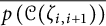 and
$\Sigma ^{\infty }_{+}$
 consists of
$p(Q)$
 ,
$p(V_{i,i+1})$
 and the orbit connecting
$p(Q)$
 and
$p(V_{i,i+1})$
 . Moreover, for the compactified vector field of system (1.3) any orbit on the cone
$p\left (\mathcal {C}(\zeta _{i,i+1})\right )$
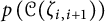 must originate from
$\overline {p(\Gamma )}$
 and tend toward
$\overline {p(\Gamma _{i,i+1})}$
 . The two orbit in
$\mathring W^{u}(p(P))$
 must be on the cones
$p\left (\mathcal {C}(\zeta _{12})\right )$
 and
$p\left (\mathcal {C}(\zeta _{23})\right )$
 , respectively, in which one tends toward the attractor
$p(V_{12})$
 and the other tends toward the attractor
$p(U_{23})$
 , because there are no other orbits of system (4.2) which emanate from F in the interior of
$S_{3}$
 except
$\zeta _{12}$
 ,
$\zeta _{23}$
 and F see Table 5
$(26a)$
 . For a given
$k\in \{1,\ 2\}$
 , let
$\xi _{k}$
 be the orbit of system (4.2) which originates from
$E_{k}$
 and tends toward F. Then the intersection of the cone
$\overline {p\left (\mathcal {C}(\xi _{k})\right )}$
 and
$\Sigma ^{\infty }_{+}$
 consists of
$p(A_{k})$
 ,
$p(Q)$
 and the orbit connecting the equilibrium
$p(A_{k})$
 and the equilibrium
$p(Q)$
 . By (4.1) it follows that for the compactified vector field of system (1.3), any orbit on the cone
$p\left (\mathcal {C}(\xi _{k})\right )$
 must originate from the
$x_{k}$
 -axis and tend toward
$\overline {p(\Gamma )}$
 . Moreover, the intersection of
$W^{u}(p(B_{k}))$
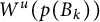 and
$p(\mathcal {C}(\xi _{k}))$
 is the orbit which emanates from
$p(B_{k})$
 and tends toward
$p(P)$
 .
For a given
$i\in \{1, 2\}$
 , each orbit in the interior of the domain limited by
$p(x_{3}=0)$
 ,
$\Sigma ^{\infty }_{+}$
 and
$p(\Gamma )\bigcup W^{u}(p(B_{i}))\bigcup p(\mathcal {C}(\zeta _{12}))\bigcup p(\mathcal {C}(\xi _{i}))$
 emanates from
$p(A_{i})$
 and tends toward
$p(V_{12})$
 . Any orbit in the interior of the domain limited by
$p(x_{i}=0)~(i=1, 2)$
 ,
$\Sigma ^{\infty }_{+}$
 and
$p(\Gamma )\bigcup W^{u}(p(B_{1}))\bigcup p(\mathcal {C}(\zeta _{23}))\bigcup p(\mathcal {C}(\xi _{1}))$
 emanates from
$p(A_{1})$
 and tends toward
$p(U_{23})$
 . The orbits in the interior of the domain limited by
$p(x_{1}=0)$
 ,
$\Sigma ^{\infty }_{+}$
 and
$p(\Gamma )\bigcup W^{u}(p(B_{2}))\bigcup p(\mathcal {C}(\zeta _{23}))\bigcup p(\mathcal {C}(\xi _{2}))$
 emanate from
$p(A_{2})$
 and tend toward
$p(U_{23})$
 . Any orbit in the interior of the domain limited by
$p(x_{i}=0)~(i= 1, 2)$
 and
$\bigcup \limits _{k=1}^{2}\big (W^{u}(p(B_{k}))\bigcup p(\mathcal {C}(\xi _{k}))\big )\bigcup p(\Gamma ) \bigcup W^{u}(p(P))$
 emanates from O and tends toward
$p(U_{23})$
 . And the orbits in the interior of the domain limited by
$p(x_{3}=0)$
 and
$\bigcup \limits _{k=1}^{2}\big (W^{u}(p(B_{k}))\bigcup p(\mathcal {C}(\xi _{k}))\big )\bigcup p(V_{12}) \bigcup p(\Gamma )\bigcup W^{u}(p(P))$
 emanate from O and tend toward
$p(V_{12})$
 . So the global phase portrait in R is that in Table 5
$(26b)$
 .
Case 42. Owing to
$J_{2}>0$
 and
$J_{i}<0~(i=1, 3)$
 , the equilibria P and Q do not exist. Referring to Tables 1 and 2,
$B_{3}$
 and
$V_{12}$
 are the attractors,
$V_{23}$
 is a repeller, and
$U_{13}$
 ,
$U_{23}$
 ,
$V_{13}$
 , and
$A_{i}~(i=1, 2, 3)$
 are saddles. From Proposition 3.3,
$\Gamma _{12}$
 is a characteristic line of
$V_{12}$
 corresponding to the eigenvalue
$\frac {I_{12}} {\alpha _1}$
 . So the phase portraits on
$\Sigma _+^{\infty }$
 ,
$p(x_{1}=0)\cap R, \ p(x_{2}=0)\cap R$
 and
$ p(x_{3}=0)\cap R $
 are those in Table 5
$(27b)$
 .
Let
$\zeta _{13}$
 be the orbit of system (4.2) which emanates from
$D_{23}$
 and tends toward
$D_{13}$
 . Then the intersection of
$\overline {p\left (\mathcal {C}(\zeta _{13})\right )}$
 and
$\Sigma ^{\infty }_{+}$
 consists of the orbit connecting
$p(V_{23})$
 and
$p(V_{13})$
 . Moreover, for the compactified vector field of system (1.3) any orbit on the cone
$p\left (\mathcal {C}(\zeta _{13})\right )$
 must originate from
$\overline {p(\Gamma _{23})}$
 and tend toward
$\overline {p(\Gamma _{13})}$
 . The two-dimensional stable manifold of
$p((U_{13}))$
 must be the cone
$\overline {p\left (\mathcal {C}(\zeta _{13})\right )}$
 , because there are no other orbits of system (4.2) which tend toward
$D_{13}$
 in the interior of
$S_{3}$
 except
$\zeta _{13}$
 see Table 5
$(27a)$
 .
Some calculations show that any orbit in the interior of the domain limited by
$p(x_{i}=0)~(i=1, 2, 3)$
 and
$p(V_{12})\bigcup W^{u}(p(U_{23}))\bigcup p(\mathcal {C}(\zeta _{13}))$
 emanates from O and tends toward
$p(V_{12})$
 , and that any orbit in the interior of the domain limited by
$p(x_{i}=0)~(i=1, 2)$
 and
$W^{u}(p(U_{23}))\bigcup p(\mathcal {C}(\zeta _{13}))$
 emanates from O and tends toward
$p(B_{3})$
 . Furthermore, any orbit in the interior of the domain limited by
$p(x_{j}=0)~(j=1, 2, 3)$
 ,
$\Sigma ^{\infty }_{+}$
 and
$W^{u}(p(U_{23}))\bigcup p(\mathcal {C}(\zeta _{13}))$
 emanates from
$p(V_{23})$
 and tends toward
$p(V_{12})$
 . All orbits in the interior of the domain limited by
$p(x_{j}=0)~(j=1, 2)$
 ,
$\Sigma ^{\infty }_{+}$
 and
$W^{u}(p(U_{23}))\bigcup p(\mathcal {C}(\zeta _{13}))$
 must emanate from
$p(V_{23})$
 and tend toward
$p(B_{3})$
 . So, the global phase portrait in R is that in Table 5
$(27b)$
 .
Case 44. By Tables 1 and 2, the equilibria P and Q exist and are saddles;
$B_{3}$
 and
$V_{12}$
 are the attractors;
$V_{13}$
 and
$V_{23}$
 are repellers; and
$A_{i}~(i=1, 2, 3)$
 ,
$U_{13}$
 and
$U_{23}$
 are saddles. From Proposition 3.3,
$\Gamma _{12}$
 is a characteristic line of
$V_{12}$
 corresponding to the eigenvalue
$\frac {I_{12}} {\alpha _1}$
 . Hence, the phase portraits on
$\Sigma _+^{\infty }$
 ,
$p(x_{1}=0)\cap R, \ p(x_{2}=0)\cap R$
 and
$ p(x_{3}=0)\cap R $
 are those in Table 5
$(28b)$
 .
For a given
$i\in \{1, 2\}$
 , we assume that
$\zeta _{i3}$
 is the orbit of system (4.2) which originates from
$D_{i3}$
 and tends toward F. The invariance of the cone
$p\left (\mathcal {C}(\zeta _{i3})\right )$
 implies that the intersection of the cone
$\overline {p\left (\mathcal {C}(\zeta _{i3})\right )}$
 and
$\Sigma ^{\infty }_{+}$
 consists of
$p(V_{i3})$
 ,
$p(Q)$
 and the orbit connecting
$p(V_{i3})$
 and
$p(Q)$
 . By (4.1) it follows that any orbit of the compactified vector field of system (1.3) on the cone
$p\left (\mathcal {C}(\zeta _{i3})\right )$
 must originate from
$\overline {p(\Gamma _{i3})}$
 and tend toward
$\overline {p(\Gamma )}$
 . Moreover,
$W^{u}(p(U_{i3}))$
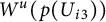 and
$p(\mathcal {C}(\zeta _{i3}))$
 must intersect along the orbit which emanates from
$p(U_{i3})$
 and tends toward
$p(P)$
 . Let
$\xi _{12}$
 resp.
$\xi _{3}$
 be the orbit of system (4.2) which originates from F and tends toward
$D_{12}$
 resp.
$E_{3}$
 . Then the intersection of the cone
$\overline {p\left (\mathcal {C}(\xi _{12})\right )}$
 resp.
$\overline {p\left (\mathcal {C}(\xi _{3})\right )}$
 and
$\Sigma ^{\infty }_{+}$
 consists of
$p(Q)$
 ,
$p(V_{12})$
 resp.
$p(A_{3})$
 and the orbit connecting
$p(Q)$
 and
$p(V_{12})$
 resp.
$p(A_{3})$
 . Furthermore, for the compactified vector field of system (1.3), any orbit on the cone
$p\left (\mathcal {C}(\xi _{12})\right )$
 resp.
$p\left (\mathcal {C}(\xi _{3})\right )$
 must originate from
$\overline {p(\Gamma )}$
 and tend toward
$\overline {p(\Gamma _{12})}$
 resp. the
$x_{3}$
 -axis. The two orbits in
$\mathring W^{u}(p(P))$
 must be on the cones
$p\left (\mathcal {C}(\xi _{12})\right )$
 and
$p\left (\mathcal {C}(\xi _{3})\right )$
 respectively, in which one tends toward the attractor
$p(V_{12})$
 and the other tends toward the attractor
$p(B_{3})$
 because there are no other orbits of system (4.2) which emanate from F in the interior of
$S_{3}$
 except
$\xi _{12}$
 ,
$\xi _{3}$
 and F see Table 5
$(28a)$
 .
For a given
$i\in \{1, 2\}$
 , each orbit in the interior of the domain limited by
$p(x_{j}=0)~(j\neq i)$
 ,
$\Sigma ^{\infty }_{+}$
 and
$p(\Gamma )\bigcup W^{u}(p(U_{i3}))\bigcup p(\mathcal {C}(\zeta _{i3}))\bigcup p(\mathcal {C}(\xi _{12}))$
 emanates from
$p(V_{i3})$
 and tends toward
$p(V_{12})$
 . Moreover, any orbit in the interior of the domain limited by
$p(\Gamma )\bigcup W^{u}(p(U_{i3}))\bigcup p(\mathcal {C}(\zeta _{i3}))\bigcup p(\mathcal {C}(\xi _{3}))$
 ,
$p(x_{j}=0)~(j\neq i, 3)$
 and
$\Sigma ^{\infty }_{+}$
 emanates from
$p(V_{i3})$
 and tends toward
$p(B_{3})$
 . And any orbit in the interior of the domain limited by
$p(x_{j}=0)~(j=1, 2, 3)$
 and
$p(V_{12})\bigcup p(\Gamma )\bigcup W^{u}(p(P)) \bigcup \bigcup \limits _{k=1}^{2}\big (W^{u}(p(U_{k3}))\bigcup p(\mathcal {C}(\zeta _{k3}))\big )$
 emanates from O and tends toward
$p(V_{12})$
 . While, all orbits in the interior of the domain limited by
$p(x_{j}=0)~(j=1, 2)$
 and
$p(\Gamma )\bigcup W^{u}(p(P))\bigcup \bigcup \limits _{k=1}^{2}\big (W^{u}(p(U_{k3}))\bigcup p(\mathcal {C}(\zeta _{k3}))\big )$
 emanate from O and tend toward
$p(B_{3})$
 . So, the global phase portrait in R is that in Table 5
$(28b)$
 .
Case 45. Owing to
$J_{2}>0$
 and
$J_{i}<0~(i=1, 3)$
 , the equilibria P and Q do not exist. Referring to Tables 1 and 2,
$V_{12}$
 is an attractor,
$A_{1}$
 and
$V_{23}$
 are repellers, and
$B_{3}$
 ,
$U_{13}$
 ,
$U_{23}$
 ,
$V_{13}$
 and
$A_{i}~(i=2, 3)$
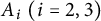 are saddles. From Proposition 3.3,
$\Gamma _{12}$
 is a characteristic line of
$V_{12}$
 corresponding to the eigenvalue
$\frac {I_{12}} {\alpha _1}$
 . By the Poincaré–Bendixson theorem and the invariance of the considered planes, we obtain easily the phase portraits on
$\Sigma _+^{\infty }$
 ,
$p(x_{1}=0)\cap R, \ p(x_{2}=0)\cap R$
 , and
$ p(x_{3}=0)\cap R $
 , which are described in Table 5
$(29b)$
 .
Let
$\zeta _{13}$
 be the orbit of system (4.2) which originates from
$D_{13}$
 and tends toward
$D_{12}$
 . Then the intersection of the cone
$\overline {p\left (\mathcal {C}(\zeta _{13})\right )}$
 and
$\Sigma ^{\infty }_{+}$
 consists of
$p(V_{13})$
 ,
$p(V_{12})$
 and the orbit connecting
$p(V_{13})$
 and
$p(V_{12})$
 . Moreover for the compactified vector field of system (1.3), any orbit on the cone
$p\left (\mathcal {C}(\zeta _{13})\right )$
 must originate from
$\overline {p(\Gamma _{13})}$
 and tend toward
$\overline {p(\Gamma _{12})}$
 , whereas the orbit passing through a point in
$\mathring W^{u}(p(U_{13}))$
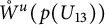 must be on the cone
$p\left (\mathcal {C}(\zeta _{13})\right )$
 and tend toward the attractor
$p(V_{12})$
 because there are no other orbits which emanates from
$D_{13}$
 in the interior of
$S_{3}$
 except
$\zeta _{13}$
 see Table 5
$(29a)$
 . The orbit passing through a point in
$W^{u}(p(U_{23}))\bigcap \mathrm {Int}R$
 must tend toward the attractor
$p(V_{12})$
 because all orbits of system (4.2) in the interior of
$S_{3}$
 which originate from
$D_{23}$
 must tend toward
$D_{12}$
 see Table 5
$(29a)$
 .
Some analysis shows that any orbit in the interior of the domain limited by
$p(x_{i}=0)~(i=1, 2, 3)$
 and
$p(V_{12})\bigcup W^{u}(p(B_{1}))\bigcup \bigcup \limits _{i=1}^{2}W^{u}(p(U_{i3}))$
 emanates from O and tends toward
$p(V_{12})$
 , and that the orbits in the interior of the domain limited by
$p(x_{i}=0)~(i=1, 2, 3)$
 ,
$\Sigma ^{\infty }_{+}$
 and
$W^{u}(p(U_{23}))\bigcup p(\mathcal {C}(\zeta _{13}))$
 emanate from
$p(V_{23})$
 and tend toward
$p(V_{12})$
 . Furthermore, the orbits in the interior of the domain limited by
$p(x_{i}=0)~(i=2, 3)$
 ,
$\Sigma ^{\infty }_{+}$
 and
$W^{u}(p(B_{1}))\bigcup p(\mathcal {C}(\zeta _{13}))$
 must emanate from
$p(A_{1})$
 and tend toward
$p(V_{12})$
 . And the equilibrium
$p(V_{12})$
 attracts all points in
$\mathrm {Int}R$
 . So, the global phase portrait in R is that in Table 5
$(29b)$
 .
Case 46. By Tables 1 and 2, it follows that the equilibria P and Q,
$B_{3}$
 ,
$U_{23}$
 ,
$V_{13}$
 , and
$A_{i}~(i=2, 3)$
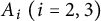 are saddles, and that
$V_{12}$
 and
$U_{13}$
 are the attractors, and
$A_{1}$
 and
$V_{23}$
 are repellers. Moreover,
$\Gamma _{12}$
 is a characteristic line of
$V_{12}$
 corresponding to the eigenvalue
$\frac {I_{12}} {\alpha _1}$
 . Hence, the phase portraits on
$\Sigma _+^{\infty }$
 ,
$p(x_{1}=0)\cap R, \ p(x_{2}=0)\cap R$
 and
$ p(x_{3}=0)\cap R $
 are those in Table 5
$(30b)$
 .
For
$j\in \{2, 3\}$
 , let
$\zeta _{1j}$
 be the orbit of system (4.2) which originates from F and tends toward
$D_{1j}$
 . Some analysis shows that the intersection of the cone
$\overline {p\left (\mathcal {C}(\zeta _{1j})\right )}$
 and
$\Sigma ^{\infty }_{+}$
 consists of
$p(Q)$
 ,
$p(V_{1j})$
 and the orbit connecting
$p(Q)$
 and
$p(V_{1j})$
 . Moreover, for the compactified vector field of system (1.3), the orbits on the cone
$p\left (\mathcal {C}(\zeta _{1j})\right )$
 must originate from
$\overline {p(\Gamma )}$
 and tend toward
$\overline {p(\Gamma _{1j})}$
 , and the two orbits in
$\mathring W^{u}(p(P))$
 must be on the cones
$p\left (\mathcal {C}(\zeta _{12})\right )$
 and
$p\left (\mathcal {C}(\zeta _{13})\right )$
 respectively, in which one tends toward the attractor
$p(V_{12})$
 and the other tends toward the attractor
$p(U_{13})$
 . Let
$\xi _{23}$
 resp.
$\xi _{1}$
 be the orbit of system (4.2) which originates from
$D_{23}$
 resp.
$E_{1}$
 and tends toward F. Then the intersection of the cone
$\overline {p\left (\mathcal {C}(\xi _{23})\right )}$
 resp.
$\overline {p\left (\mathcal {C}(\xi _{1})\right )}$
 and
$\Sigma ^{\infty }_{+}$
 consists of
$p(V_{23})$
 resp.
$p(A_{1})$
 ,
$p(Q)$
 and the orbit connecting
$p(V_{23})$
 resp.
$p(A_{1})$
 and
$p(Q)$
 . Moreover, any orbit of the compactified vector field of system (1.3) on the cone
$p\left (\mathcal {C}(\xi _{23})\right )$
 resp.
$p\left (\mathcal {C}(\xi _{1})\right )$
 must originate from
$\overline {p(\Gamma _{23})}$
 resp. the
$x_{1}$
 -axis and tend toward
$\overline {p(\Gamma )}$
 . Further calculations show that
$W^{u}(p(U_{23}))$
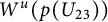 and
$p(\mathcal {C}(\xi _{23}))$
 intersect along the orbit which emanates from
$p(U_{23})$
 and tends toward
$p(P)$
 , and that
$W^{u}(p(B_{1}))$
 and
$p(\mathcal {C}(\xi _{1}))$
 intersect along the orbit which emanates from
$p(B_{1})$
 and tends toward
$p(P)$
 .
One can check that any orbit in the interior of the domain limited by
$p(x_{i}=0)~(i=1, 2)$
 ,
$\Sigma ^{\infty }_{+}$
 and
$p(\Gamma )\bigcup W^{u}(p(U_{23}))\bigcup p(\mathcal {C}(\zeta _{13}))\bigcup p(\mathcal {C}(\xi _{23}))$
 emanates from
$p(V_{23})$
 and tends toward
$p(U_{13})$
 , and that any orbit in the interior of the domain limited by
$p(\Gamma )\bigcup W^{u}(p(U_{23}))\bigcup p(\mathcal {C}(\zeta _{12}))\bigcup p(\mathcal {C}(\xi _{23}))$
 ,
$p(x_{i}=0)~(i=1, 3)$
 and
$\Sigma ^{\infty }_{+}$
 emanates from
$p(V_{23})$
 and tends toward
$p(V_{12})$
 . The orbits in the interior of the domain limited by
$p(\Gamma )\bigcup W^{u}(p(B_{1}))\bigcup p(\mathcal {C}(\zeta _{13}))\bigcup p(\mathcal {C}(\xi _{1}))$
 ,
$p(x_{2}=0)$
 and
$\Sigma ^{\infty }_{+}$
 must emanate from
$p(A_{1})$
 and tend toward
$p(U_{13})$
 . The orbits in the interior of the domain limited by
$p(\Gamma )\bigcup W^{u}(p(B_{1}))\bigcup p(\mathcal {C}(\zeta _{12}))\bigcup p(\mathcal {C}(\xi _{1}))$
 ,
$p(x_{3}=0)$
 and
$\Sigma ^{\infty }_{+}$
 emanate from
$p(A_{1})$
 and tend toward
$p(V_{12})$
 . Moreover, the orbits in the interior of the domain limited by
$p(x_{i}=0)~(i=1, 2)$
 and
$p(\Gamma )\bigcup W^{u}(p(P))\bigcup W^{u}(p(B_{1}))\bigcup W^{u}(p(U_{23}))\bigcup p(\mathcal {C}(\xi _{23}))\bigcup p(\mathcal {C}(\xi _{1}))$
 move away from O and tend toward
$p(U_{13})$
 , and the orbits in the interior of the domain limited by
$p(V_{12})\bigcup p(\Gamma )\bigcup W^{u}(p(P)) \bigcup W^{u}(p(B_{1}))\bigcup W^{u}(p(U_{23}))\bigcup p(\mathcal {C}(\xi _{23}))\bigcup p(\mathcal {C}(\xi _{1}))$
 and
$p(x_{i}=0)~(i=1, 3)$
 emanate from O and tend toward
$p(V_{12})$
 . So, the global phase portrait in R is that in Table 5
$(30b)$
 .
Case 47. Because of
$J_{i}<0~(i=1, 2)$
 and
$J_{3}>0 $
 , the equilibria P and Q do not exist. Referring to Tables 1 and 2,
$B_{3}$
 is an attractor,
$A_{i}~(i=1, 2)$
 are the repellers, and
$A_{3}$
 and
$V_{12}$
 are saddles. From Proposition 3.3,
$\Gamma _{12}$
 is a characteristic line of
$V_{12}$
 corresponding to the eigenvalue
$\frac {I_{12}} {\alpha _1}$
 . Hence, the phase portraits on
$\Sigma _+^{\infty }$
 ,
$p(x_{1}=0)\cap R, \ p(x_{2}=0)\cap R$
 and
$ p(x_{3}=0)\cap R $
 are those in Table 5
$(31b)$
 .
One can check that any orbit in the interior of the domain limited by
$p(x_{i}=0)~(i=1, 2, 3)$
 and
$W^{u}(p(A_{3}))\bigcup \bigcup \limits _{k=1}^{2} W^{u}(p(B_{k}))\bigcup W^{u}(p(V_{12}))$
 emanates from O and tends toward
$p(B_{3})$
 . Moreover, for a given
$i\in \{1, 2\}$
 , each orbit in the interior of the domain limited by
$W^{u}(p(A_{3}))\bigcup W^{u}(p(B_{i}))\bigcup W^{u}(p(V_{12}))$
 ,
$p(x_{j}=0)~(j\neq i)$
 and
$\Sigma _+^{\infty }$
 emanates from
$p(A_{i})$
 and tends toward
$p(B_{3})$
 . The equilibrium
$p(B_{3})$
 attracts all points in
$\mathrm {Int}R$
 . So, the global phase portrait in R is that in Table 5
$(31b)$
 .
Case 48. Referring to Tables 1 and 2, it follows that P and Q exist and are saddles, and
$A_{3}$
 is a saddle, and that
$B_{3}$
 and
$V_{12}$
 are the attractors, and
$A_{i}~(i=1, 2)$
 are repellers. Moreover,
$\Gamma _{12}$
 is a characteristic line of
$V_{12}$
 corresponding to the eigenvalue
$\frac {I_{12}} {\alpha _1}$
 . So, the phase portraits on
$\Sigma _+^{\infty }$
 ,
$p(x_{1}=0)\cap R, \ p(x_{2}=0)\cap R$
 and
$ p(x_{3}=0)\cap R $
 are those in Table 5
$(32b)$
 .
Let
$\zeta _{i}$
 ,
$i\in \{1, 2\}$
 , be the orbits of system (4.2) which originate from
$E_{i}$
 and tend toward F. Then the intersection of the cone
$\overline {p\left (\mathcal {C}(\zeta _{i})\right )}$
 and
$\Sigma ^{\infty }_{+}$
 consists of
$p(A_{i})$
 ,
$p(Q)$
 and the orbit connecting
$p(A_{i})$
 and
$p(Q)$
 . Moreover, the orbits of the compactified vector field of system (1.3) on the cone
$p\left (\mathcal {C}(\zeta _{i})\right )$
 must originate from the
$x_{i}$
 -axis and tend toward
$\overline {p(\Gamma )}$
 , and
$W^{u}(p(B_{i}))$
 and
$p(\mathcal {C}(\zeta _{i}))$
 must intersect along the orbit which emanates from
$p(B_{i})$
 and tends toward
$p(P)$
 . Let
$\xi _{12}$
 resp.
$\xi _{3}$
 be the orbit of system (4.2) which originates from F and tends toward
$D_{12}$
 resp.
$E_{3}$
 . Then the intersection of the cone
$\overline {p\left (\mathcal {C}(\xi _{12})\right )}$
 resp.
$\overline {p\left (\mathcal {C}(\xi _{3})\right )}$
 and
$\Sigma ^{\infty }_{+}$
 consists of
$p(Q)$
 ,
$p(V_{12})$
 resp.
$p(A_{3})$
 and the orbit connecting
$p(Q)$
 and
$p(V_{12})$
 resp.
$p(A_{3})$
 . Furthermore, for the compactified vector field of system (1.3), any orbit on the cone
$p\left (\mathcal {C}(\xi _{12})\right )$
 resp.
$p\left (\mathcal {C}(\xi _{3})\right )$
 must originate from
$\overline {p(\Gamma )}$
 and tend toward
$\overline {p(\Gamma _{12})}$
 resp. the
$x_{3}$
 -axis. And its two orbits in
$\mathring W^{u}(p(P))$
 must be on the cones
$p\left (\mathcal {C}(\xi _{12})\right )$
 and
$p\left (\mathcal {C}(\xi _{3})\right )$
 , respectively, and they tend toward respectively the attractors
$p(V_{12})$
 and
$p(B_{3})$
 .
Some analysis shows that any orbit in the interior of the domain limited by
$p(x_{j}=0)~(j=1, 2)$
 and
$p(\Gamma )\bigcup W^{u}(p(P))\bigcup \bigcup \limits _{k=1}^{2}\big (W^{u}(p(B_{k}))\bigcup p(\mathcal {C}(\zeta _{k}))\big )$
 originates from O and tends toward
$p(B_{3})$
 , and that the orbits in the interior of the domain limited by
$p(V_{12})\bigcup p(\Gamma ) \bigcup W^{u}(p(P))\bigcup \bigcup \limits _{k=1}^{2}\big (W^{u}(p(B_{k}))\bigcup p(\mathcal {C}(\zeta _{k}))\big )$
 and
$p(x_{3}=0)$
 emanate from O and tend toward
$p(V_{12})$
 . Moreover, for
$i\in \{1, 2\}$
 , one can check that each orbit in the interior of the domain limited by
$ p(\Gamma )\bigcup W^{u}(p(B_{i}))\bigcup p(\mathcal {C}(\zeta _{i}))\bigcup p(\mathcal {C}(\xi _{12}))$
 ,
$p(x_{3}=0)$
 and
$\Sigma ^{\infty }_{+}$
 emanates from
$p(A_{i})$
 and tends toward
$p(V_{12})$
 , and that all orbits in the interior of the domain limited by
$p(\Gamma )\bigcup W^{u}(p(B_{i}))\bigcup p(\mathcal {C}(\zeta _{i}))\bigcup p(\mathcal {C}(\xi _{3}))$
 ,
$p(x_{j}=0)~(j\neq i, 3)$
 and
$\Sigma ^{\infty }_{+}$
 emanate from
$p(A_{i})$
 and tend toward
$p(B_{3})$
 . So, the global phase portrait in R is that in Table 5
$(32b)$
 .
Case 49. Because
$J_{i}~(i=1, 2, 3)$
 have different signs, it follows from Tables 1 and 2 that the equilibria P and Q do not exist, and that
$V_{12}$
 is an attractor,
$A_{3}$
 is a repeller, and
$B_{3}$
 and
$A_{i}~(i=1, 2)$
 are saddles. Proposition 3.3 implies that
$\Gamma _{12}$
 is a characteristic line of
$V_{12}$
 corresponding to the eigenvalue
$\frac {I_{12}} {\alpha _1}$
 . Hence, the phase portraits on
$\Sigma _+^{\infty }$
 ,
$p(x_{1}=0)\cap R, \ p(x_{2}=0)\cap R$
 and
$ p(x_{3}=0)\cap R $
 are those in Table 5
$(33b)$
 .
Further calculations show that any orbit in the interior of the domain limited by
$p(x_{j}=0)~(j=1, 2, 3)$
 and
$p(V_{12})\bigcup W^{u}(p(B_{3})) $
 originates from O and tends toward
$p(V_{12})$
 , and that any orbit in the interior of the domain limited by
$ W^{u}(p(B_{3}))$
 ,
$p(x_{j}=0)~(j=1, 2, 3)$
 and
$\Sigma ^{\infty }_{+}$
 emanates from
$p(A_{3})$
 and tends toward
$p(V_{12})$
 . The fact that the equilibrium
$p(V_{12})$
 is a global attractor in
$\mathrm {Int}R$
 induces that the global phase portrait in R is that in Table 5
$(33b)$
 .
Case 52. It follows from
$J_{i}>0~(i=1, 2, 3)$
 and
$\Phi <0$
 that the positive finite equilibrium P and the positive equilibrium at infinity Q both exist. The former is an attractor and the latter is a saddle whose stable manifold is located in the positive plane at infinity and its unstable manifold lies on the ray
$\Gamma $
 in between P and Q. By Tables 1 and 2,
$B_{3}$
 ,
$U_{13}$
 ,
$U_{23}$
 ,
$V_{12}$
 ,
$V_{13}$
 , and
$V_{23}$
 are saddles. From Proposition 3.3,
$\Gamma _{12}$
 is a characteristic line of
$V_{12}$
 corresponding to the eigenvalue
$\frac {I_{12}} {\alpha _1}$
 . Hence, the phase portraits on
$\Sigma _+^{\infty }$
 ,
$p(x_{1}=0)\cap R, \ p(x_{2}=0)\cap R$
 and
$ p(x_{3}=0)\cap R $
 are those in Table 5
$(34b)$
 .
For
$i\in \{1, 2\}$
 , let
$\zeta _{i3}$
 be the orbit of system (4.2) which originates from
$D_{i3}$
 and tends toward F. Then the intersection of the cone
$\overline {p\left (\mathcal {C}(\zeta _{i3})\right )}$
 and
$\Sigma ^{\infty }_{+}$
 consists of
$p(V_{i3})$
 ,
$p(Q)$
 and the orbit connecting
$p(V_{i3})$
 and
$p(Q)$
 . Moreover, for the compactified vector field of system (1.3), it follows from (4.1) that any orbit on the cone
$p\left (\mathcal {C}(\zeta _{i3})\right )$
 must originate from
$\overline {p(\Gamma _{i3})}$
 and tend toward
$\overline {p(\Gamma )}$
 , and that any orbit passing through a point in
$\mathring W^{u}(p(U_{i3}))$
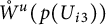 must be on the cone
$p\left (\mathcal {C}(\zeta _{i3})\right )$
 and tend toward the attractor
$p(P)$
 .
Now the orbits in the interior of the domain limited by
$p(x_{i}=0)~(i=1, 2, 3)$
 and
$p(P)\bigcup \bigcup \limits _{k=1}^{3} W^{u}(p(B_{k}))\bigcup \bigcup \limits _{i=1}^{2}W^{u}(p(U_{i3}))\bigcup W^{u}(p(V_{12}))\bigcup W^{u}(p(Q))$
 emanate from O and tend toward
$p(P)$
 . And the orbits in the interior of the domain limited by
$p(x_{j}=0)~(j=1, 2)$
 ,
$\Sigma ^{\infty }_{+}$
 and
$p(\Gamma )\bigcup W^{u}(p(B_{3}))\bigcup \bigcup \limits _{i=1}^{2}p(\mathcal {C}(\zeta _{i3}))$
 emanates from
$p(A_{3})$
 and tends toward
$p(P)$
 . Moreover, one can verify that for
$i\in \{1, 2\}$
 , each orbit in the interior of the domain limited by
$p(x_{j}=0)~(j\neq i)$
 ,
$\Sigma ^{\infty }_{+}$
 and
$p(P)\bigcup W^{u}(p(B_{i}))\bigcup p(\mathcal {C}(\zeta _{i3}))\bigcup W^{u}(p(V_{12}))\bigcup W^{u}(p(Q))$
 emanates from
$p(A_{i})$
 and tends toward
$p(P)$
 , and that the equilibrium
$p(P)$
 is the global attractor in
$\mathrm {Int}R$
 . So, the global phase portrait in R is that in Table 5
$(34b)$
 .
Case 53. Owing to
$J_{i}>0~(i=1, 2)$
 and
$J_{3}<0$
 , the equilibria P and Q do not exist. Referring to Tables 1 and 2,
$V_{12}$
 is an attractor,
$A_{i}~(i=1, 2, 3)$
 are repellers, and
$B_{3}$
 ,
$U_{13}$
 ,
$U_{23}$
 ,
$V_{13}$
 and
$V_{23}$
 are saddles. By Proposition 3.3, it follows that
$\Gamma _{12}$
 is a characteristic line of
$V_{12}$
 corresponding to the eigenvalue
$\frac {I_{12}}{\alpha _1}$
 . So, the phase portraits on
$\Sigma _+^{\infty }$
 ,
$p(x_{1}=0)\cap R, \ p(x_{2}=0)\cap R$
 and
$ p(x_{3}=0)\cap R $
 are those in Table 5
$(35b)$
 .
For
$i\in \{1, 2\}$
 , let
$\zeta _{i3}$
 be the orbit of system (4.2) which emanates from
$D_{i3}$
 and tends toward
$D_{12}$
 . Then the intersection of
$\overline {p\left (\mathcal {C}(\zeta _{i3})\right )}$
 and
$\Sigma ^{\infty }_{+}$
 consists of
$p(V_{i3})$
 ,
$p(V_{12})$
 and the orbit connecting
$p(V_{i3})$
 and
$p(V_{12})$
 . Moreover, for the compactified vector field of system (1.3), it follows from (4.1) that any orbit on the cone
$p\left (\mathcal {C}(\zeta _{i3})\right )$
 must originate from
$\overline {p(\Gamma _{i3})}$
 and tend toward
$\overline {p(\Gamma _{12})}$
 , and that any orbit passing through a point in
$\mathring W^{u}(p(U_{i3}))$
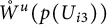 must be on the cone
$p\left (\mathcal {C}(\zeta _{i3})\right )$
 and tend toward the attractor
$p(V_{12})$
 .
Further analysis shows that all orbits in the interior of the domain limited by
$p(x_{i}=0)~(i=1, 2, 3)$
 and
$p(V_{12})\bigcup \bigcup \limits _{k=1}^{3}W^{u}(p(B_{k}))\bigcup \bigcup \limits _{i=1}^{2}W^{u}(p(U_{i3}))$
 emanate from O and tend toward
$p(V_{12})$
 . Moreover, for
$i\in \{1, 2\}$
 , each orbit in the interior of the domain limited by
$p(x_{j}=0)~(j\neq i)$
 ,
$\Sigma ^{\infty }_{+}$
 and
$W^{u}(p(B_{i}))\bigcup p(\mathcal {C}(\zeta _{i3}))$
 emanates from
$p(A_{i})$
 and tends toward
$p(V_{12})$
 . Any orbit in the interior of the domain limited by
$p(x_{j}=0)~(j=1, 2)$
 ,
$\Sigma ^{\infty }_{+}$
 and
$W^{u}(p(B_{3}))\bigcup \bigcup \limits _{i=1}^{2}p(\mathcal {C}(\zeta _{i3}))$
 emanates from
$p(A_{3})$
 and tends toward
$p(V_{12})$
 . Since the equilibrium
$p(V_{12})$
 is the global attractor in
$\mathrm {Int}R$
 , the global phase portrait in R is that in Table 5
$(35b)$
 .
So far, we have analyzed all the possible cases, and obtained exactly 35 topologically different dynamical classes for the compactified vector field associated with system (1.3) restricted to R, which are shown in Table 5.
It completes the proof of Theorems 2.1–2.8.
Proof of Theorem 2.9
Throughout the above analysis, one gets that only for the classes 1–17 whose
$2\times 2$
 principal minor
$I_{12}$
 of the coefficient matrix A is positive, all positive trajectories of the three-dimensional type-K monotone Lotka–Volterra system (1.3) are bounded in
$\mathbb {R}^{3}_{+}$
 (see the blue figures in Table 5). For the other classes, the
$2\times 2$
 principal minor
$I_{12}$
 of A is less than zero. The proof is done.
We remark that this is the second one of a series works on the topological classification of three-dimensional Lotka–Volterra systems with the identical intrinsic growth. The first one in [Reference Liang, Jiang and Zhang6] completed the global topological classification of the cooperative Lotka–Volterra system with the identical intrinsic growth. The coming works are in plan to classify global topological dynamics of the type-K competitive, prey-predator Lotka–Volterra systems with the identical intrinsic growth.