2. Description of the geometry and the plasma

We consider a cylindrical plasma filament, with spatially homogeneous density, embedded in a uniform background plasma. The filament has a circular cross-section with its axis aligned along the ambient magnetic field line (figure 1). The axial extent of the filament is taken to be infinite, which allows us to neglect the effects of the end caps. Inherent in this assumption is that the RF fields are axially confined to a spatial region that is smaller than the length of the filament. The magnetic field in the scattering region is uniform and the plasma is presumed to be cold.

Figure 1.

The cylindrical coordinate system: the ambient magnetic field is along the axial direction $\hat {\boldsymbol {z}}$; $\hat {\boldsymbol {\rho }}$ and $\hat {\boldsymbol {\phi }}$ are the unit vectors along the radial and azimuthal directions, respectively.

The relationship between the cylindrical coordinate system $(\hat {\boldsymbol {\rho }},\, \hat {\boldsymbol {\phi }},\, \hat {\boldsymbol {z}})$, used as a basis in the theory, and the Cartesian coordinate system $(\hat {\boldsymbol {x}},\, \hat {\boldsymbol {y}},\, \hat {\boldsymbol {z}})$ can be expressed in the form taken by the position vector $\boldsymbol {r}$,

(2.1)\begin{equation} \boldsymbol{r} = x \, \hat{\boldsymbol{x}} + y \; \hat{\boldsymbol{y}} + z \, \hat{\boldsymbol{z}} = \rho \, \hat{\boldsymbol{\rho}} + z \, \hat{\boldsymbol{z}}, \end{equation}

where $\rho = \sqrt {x^{2} +y^{2}}$, and $z$ is along the axial direction. The origin of the coordinate system is the centre of the cylindrical filament.

3. Propagation of electromagnetic waves in a plasma

The mathematical description of the propagation and scattering of RF waves in a cold plasma is based on the linearized set of continuity and momentum fluid equations for electrons and ions. These are combined with Faraday's and Ampere's equations (Stix Reference Stix1992; Ram & Hizanidis Reference Ram and Hizanidis2016) to obtain the spatial variation of the RF electric field,

(3.1)\begin{equation} \boldsymbol{\nabla} \boldsymbol{\times} \left\{ \boldsymbol{\nabla} \boldsymbol{\times} \, \boldsymbol{E} \left( \boldsymbol{r} \right) \right\} - \frac{\omega^{2}}{c^{2}} \ \boldsymbol{\mathsf{K}} \left( \boldsymbol{r} \right) \boldsymbol{\cdot} \boldsymbol{E} \left( \boldsymbol{r} \right) = 0, \end{equation}

where $\omega$ is the angular frequency of the electromagnetic fields, $c$ is the speed of light and $\boldsymbol{\mathsf{K}} ( \boldsymbol {r} )$ is the plasma permittivity tensor. We have assumed that the plasma equilibrium is time independent, while the linearized perturbed electromagnetic fields have a time dependence of the form ${\rm e}^{-\textrm {i} \omega t}$, where $t$ is the time. In the cylindrical coordinate system where the ambient magnetic field is $\boldsymbol {B}_0 = B_0 \, \hat {\boldsymbol {z}}$, and $\boldsymbol{\mathsf{K}} ( \boldsymbol {r} )$ has the form (Stix Reference Stix1992),

(3.2)\begin{equation} \boldsymbol{\mathsf{K}} = \left( \begin{array}{@{}ccccc@{}} K_\rho & \ \ & -\textrm{i} K_\phi & \ \ & 0 \\ \\ \textrm{i}K_\phi & \ \ & K_\rho & \ \ & 0 \\ \\ 0 & \ \ & 0 & \ \ & K_z \end{array} \right), \end{equation}

where

(3.3)\begin{equation} \left. \begin{aligned} K_\rho & = 1 - \frac{\omega_{pe}^{2}}{\omega^{2}-\omega_{ce}^{2}} - \sum_{i} \ \frac{\omega_{pi}^{2}}{\omega^{2}-\omega_{ci}^{2}}, \\ K_\phi & ={-} \frac{\omega_{ce}}{\omega} \ \frac{\omega_{pe}^{2}}{\omega^{2}-\omega_{ce}^{2}} + \sum_{i} \ \frac{\omega_{ci}}{\omega} \ \frac{\omega_{pi}^{2}}{\omega^{2}-\omega_{ci}^{2}}, \\ K_z & = 1 - \frac{\omega_{pe}^{2}}{\omega^{2}} -\sum_{i} \ \frac{\omega_{pi}^{2}}{\omega^{2}}, \end{aligned} \right\} \end{equation}

$\omega _{pe}$ ($\omega _{pi}$) and $\omega _{ce}$ ($\omega _{ci}$) are the angular electron (ion) plasma frequency and cyclotron frequency, respectively, and the index $i$ represents all the ion species in the plasma. The plasma and cyclotron frequencies can, in general, be functions of space. The permittivity tensor of the background plasma and of the filament are expressed in terms of their respective ion compositions and constant, but different, densities. Subsequently, the elements of $\boldsymbol{\mathsf{K}}$ are constants in each region inside and outside the filament.

For a spatially independent $\boldsymbol{\mathsf{K}}$, (3.1) has the form of a vector Helmholtz equation and can be solved analytically in the cylindrical coordinate system using vector cylinder functions (Ram & Hizanidis Reference Ram and Hizanidis2016). We assume that the incoming RF wave launched by an antenna is a plane electromagnetic wave of fixed frequency. In addition, we assume that the component of the wave vector along the direction of the ambient magnetic field $k_z$ is prescribed ab initio. As the axis of the cylindrical filament is also aligned along the magnetic field, boundary conditions imposed by Maxwell's equations require that $k_z$ be the same for all waves: those inside the filament and those that are scattered. This property leads to some simplification when solving (3.1) (Ram & Hizanidis Reference Ram and Hizanidis2016).

In § 4 we derive, in cylindrical coordinates, the necessary properties of the plane wave that are consistent with (3.1). A description of the scattered waves and the waves inside the filament is outlined in § 4.

4. Dispersion characteristics and polarization of a plane plasma wave

In cylindrical coordinates, the spatial variation of a plane wave is (Stratton Reference Stratton1941),

(4.1)\begin{equation} {\rm e}^{\textrm{i} \boldsymbol{k} \boldsymbol{\cdot} \boldsymbol{r}} = \exp({{\textrm{i} k_\rho \rho \cos \left( \phi - \phi_k \right) + \textrm{i} k_z z}}) = \sum_{m={-}\infty}^{\infty} \ i^{m} \ {\text J}_m \left( k_\rho \rho \right) \exp({{ \textrm{i} m \left( \phi - \phi_k \right)}}) \exp({\textrm{i} k_z z}), \end{equation}

where ${\text J}_m$ is the Bessel function of the first kind of order $m$, $\phi$ and $\phi _k$ are the azimuthal angles between the $x$-axis and $\boldsymbol {r}$ and $\boldsymbol {k}$, respectively, and $k_\rho = \sqrt {k_x^{2}+k_y^{2}}$ with $\boldsymbol {k} = k_x \, \hat {\boldsymbol {x}} + k_y \, \hat {\boldsymbol {y}} + k_z \, \hat {\boldsymbol {z}}$.

In the cylindrical coordinate system (Ram & Hizanidis Reference Ram and Hizanidis2016),

(4.2)\begin{equation} \left( \begin{array}{c} \hat{\boldsymbol{\rho}}\\ \hat{\boldsymbol{\phi}}\\ \hat{\boldsymbol{z}} \end{array} \right) \exp({\textrm{i} \boldsymbol{k} \boldsymbol{\cdot} \boldsymbol{r} }) = \sum_{m={-}\infty}^{\infty} \ \textrm{i}^{m} \exp({-\textrm{i}m \phi_k}) \left( \boldsymbol{a} \boldsymbol{l}_{m} + \boldsymbol{b} \boldsymbol{m}_{m} + \boldsymbol{c} \boldsymbol{n}_{m} \right). \end{equation}

The right-hand side is a sum of three dyadics, with

(4.3)\begin{equation} \left. \begin{aligned} \boldsymbol{a} & = \frac{\textrm{i}}{k^{2}} \ \left( \begin{array}{c} - k_\rho \cos \left( \phi - \phi_k \right) \\ k_\rho \sin \left( \phi - \phi_k \right) \\ -k_z \end{array} \right), \\ \boldsymbol{b} & = \frac{\textrm{i}}{k_\rho} \ \left( \begin{array}{c} \sin \left( \phi - \phi_k \right) \\ \cos \left( \phi - \phi_k \right) \\ 0 \end{array} \right),\\ \boldsymbol{c} & = \frac{1}{k k_\rho} \ \left( \begin{array}{c} - k_z \cos \left( \phi - \phi_k \right) \\ k_z \sin \left( \phi - \phi_k \right) \\ k_\rho \end{array} \right). \end{aligned} \right\} \end{equation}

The vector cylinder functions $\boldsymbol {l}_{m}$, $\boldsymbol {m}_{m}$ and $\boldsymbol {n}_{m}$ are (Stratton Reference Stratton1941)

(4.4)\begin{equation} \left. \begin{aligned} \boldsymbol{l}_m \left( \rho, \phi, z; k_\rho, k_z \right) & = \left[ \left( \frac{\partial}{\partial \rho} {\text J}_m \right) \hat{\boldsymbol{\rho}} + \left\{ \frac{\textrm{i}m}{\rho} \hat{\boldsymbol{\phi}} + \textrm{i} k_z \ \hat{\boldsymbol{z}} \right\} {\text J}_m \right] \exp({\textrm{i} k_z z + \textrm{i} m \phi}), \\ \boldsymbol{m}_m \left( \rho, \phi, z; k_\rho, k_z \right) & = \left[ \frac{\textrm{i}m}{\rho} {\text J}_m \ \hat{\boldsymbol{\rho}} - \left( \frac{\partial}{\partial \rho} {\text J}_m \right) \hat{\boldsymbol{\phi}} \right] \exp({\textrm{i} k_z z + \textrm{i} m \phi}), \\ \boldsymbol{n}_m \left( \rho, \phi, z; k_\rho, k_z \right) & = \left[ \frac{\textrm{i}k_z}{k} \left( \frac{\partial}{\partial \rho} {\text J}_m \right) \hat{\boldsymbol{\rho}} - \left\{ \frac{k_z}{k} \frac{m}{\rho} \hat{\boldsymbol{\phi}} - \frac{k_\rho^{2}}{k} \hat{\boldsymbol{z}} \right\} {\text J}_m \right] \exp({\textrm{i} k_z z + \textrm{i} m \phi}), \end{aligned} \right\} \end{equation}

where the argument of ${\text J}_m$ is $k_\rho \rho$.

For a plane wave the electric field is

(4.5)\begin{equation} \boldsymbol{E}_P \left( \boldsymbol{r} \right) = \boldsymbol{E}_0 \left( \boldsymbol{k}, \omega \right) \exp({\textrm{i} \boldsymbol{k} \boldsymbol{\cdot} \boldsymbol{r}}), \end{equation}

where $\boldsymbol {E}_0$ is the electric field vector which is independent of space and time. Substituting this form into (3.1) yields

(4.6)\begin{equation} \boldsymbol{\mathsf{D}} \left(\boldsymbol{k}, \omega \right) \boldsymbol{\cdot} \boldsymbol{E}_0 \left( \boldsymbol{k}, \omega \right) = 0, \end{equation}

where

(4.7)\begin{equation} \boldsymbol{\mathsf{D}} \left( \boldsymbol{k}, \omega \right) = \frac{c^{2}}{\omega^{2}} \left( \boldsymbol{k} \boldsymbol{k} - k^{2} \boldsymbol{\mathsf{I}} \right) + \boldsymbol{\mathsf{K}}. \end{equation}

Here $\boldsymbol {k} \boldsymbol {k}$ is a dyadic and $\boldsymbol{\mathsf{I}}$ is the identity tensor. For a non-zero electric field of the RF wave, we require that

(4.8)\begin{equation} \textrm{det} \left( \boldsymbol{\mathsf{D}} \left( \boldsymbol{k}, \omega \right) \right) = 0, \end{equation}

where det denotes the determinant of the tensor. Using (4.7) in (4.8) leads to the following algebraic equation:

(4.9)\begin{equation} n_{\rho}^{4} K_{\rho} + n_{\rho}^{2} [ K_{\phi}^{2} - \left( K_{ \rho} + K_{z} \right) \left( K_{\rho} - n_{z}^{2} \right) ] + K_{z} [ \left( K_{\rho} - n_{z}^{2} \right)^{2} - K_{\phi}^{2} ] = 0, \end{equation}

where the index of refraction $\boldsymbol {n}=c\boldsymbol {k}/\omega$.

For a prescribed $n_z$, the two solutions of the bi-quadratic equation are

(4.10)\begin{align} n_{\rho \pm}^{2} &= \frac{1}{2K_{\rho}} \left( K_{\rho} + K_{z} \right) \left( K_{\rho} - n_{z}^{2} \right) - \frac{1}{2K_{\rho}} K_{\phi}^{2} \nonumber\\ &\quad \pm \frac{1}{2K_{\rho}} \ \sqrt{ \left[ \left\{ \left(K_{\rho} - K_{z} \right) \left( K_{\rho} - n_{z}^{2} \right) - K_{\phi}^{2} \right\}^{2} + 4 n_{z}^{2} K_{\phi}^{2} K_{z} \right] }. \end{align}

We associate one of the roots to a slow wave and the other to a fast wave depending on their relative phase velocities. The association will become clear when we consider specific examples.

4.1. Electric field polarizations

The electric field $\boldsymbol {E}_0$ in (4.5) can be written as

(4.11)\begin{equation} \boldsymbol{E}_0 ( \boldsymbol{k}, \omega ) = {\mathcal{E}_0}( E_{k \rho} \, \hat{\boldsymbol{\rho}}_k + E_{k \phi} \, \hat{\boldsymbol{\phi}}_k + E_{k z} \, \hat{\boldsymbol{z}}), \end{equation}

where $\mathcal {E}_0$ is the amplitude of the electric field, and $( E_{k \rho }, E_{k \phi }, E_{k z} )$ are the components of the polarization vector along $( \hat {\boldsymbol {\rho }}_k, \hat {\boldsymbol {\phi }}_k, \hat {\boldsymbol {z}} )$. The directional vector $( \hat {\boldsymbol {\rho }}_k, \hat {\boldsymbol {\phi }}_k, \hat {\boldsymbol {z}} )$ is in the cylindrical coordinate system defined in the wave vector space.

The polarization of the wave electric field follows from (4.6). Depending on whether the wave is a slow wave or a fast wave, we will make use of one of the following two representations for the polarization:

(4.12)\begin{equation} \left. \begin{aligned} e_{k \rho} & ={-} \frac{n_{\rho } n_{z} \left( K_{\rho} - n_{\rho}^{2} - n_{z}^{2} \right)}{\left( K_{\rho} -n_{z}^{2} \right) \left( K_{\rho} - n_{\rho}^{2} - n_{z}^{2} \right) - K_{\phi}^{2}}, \\ e_{k \phi} & ={-} \frac{\textrm{i} n_{\rho} n_{z} K_{\phi}} {\left( K_{\rho} -n_{z}^{2} \right) \left( K_{\rho} - n_{\rho}^{2} - n_{z}^{2} \right) - K_{\phi}^{2}}, \\ e_{k z} & = 1, \end{aligned} \right\} \end{equation}

or

(4.13)\begin{equation} \left. \begin{aligned} e_{k \rho} & = 1, \\ e_{k \phi} & ={-} \frac{\textrm{i} K_{\phi}}{K_{\rho} - n_{\rho}^{2} - n_{z}^{2}}, \\ e_{k z} & ={-} \frac{n_{\rho} n_{z}}{K_{z} - n_{\rho}^{2}}, \end{aligned} \right\} \end{equation}

where $n_\rho$ is one of the roots given in (4.10). For the slow wave (4.12) is a useful form for the polarization vectors, while (4.13) is appropriate for the fast wave. The components $( E_{k \rho }, E_{k \phi }, E_{k z} )$ in (4.11) are defined as

(4.14)\begin{equation} \left( E_{k \rho}, \, E_{k \phi}, \, E_{k z} \right) = \dfrac{1}{\sqrt{ \left| e_{k \rho} \right| ^{2} + \left| e_{k \phi} \right| ^{2} + \left| e_{k z} \right| ^{2} }} \ \left( e_{k \rho},\, e_{k \phi},\, e_{k z} \right). \end{equation}

4.2. Electric field representation of a plane wave in cylindrical coordinates

In the wave vector space,

(4.15) \begin{equation} \left( \begin{array}{@{}c@{}} \hat{\boldsymbol{\rho}}_k\\ \hat{\boldsymbol{\phi}}_k\\ \hat{\boldsymbol{z}} \end{array} \right) \exp({\textrm{i} \boldsymbol{k} \boldsymbol{\cdot} \boldsymbol{r} }) = \sum_{m={-}\infty}^{\infty} \, i^{m} \ \exp({-\textrm{i}m \phi_k}) \ \left(\boldsymbol{a}_k \boldsymbol{l}_{m} + \boldsymbol{b}_k \boldsymbol{m}_{m} + \boldsymbol{c}_k \boldsymbol{n}_{m} \right), \end{equation}

where

(4.16a–c) \begin{equation} \boldsymbol{a}_k = \frac{\textrm{i}}{k^{2}} \ \left( \begin{array}{@{}c@{}} - k_\rho \\ 0 \\ -k_z \end{array} \right),\quad \boldsymbol{b}_k = \frac{\textrm{i}}{k_\rho} \ \left( \begin{array}{@{}c@{}} 0 \\ 1 \\ 0 \end{array} \right), \quad \boldsymbol{c}_k = \frac{1}{k k_\rho} \ \left( \begin{array}{@{}c@{}} - k_z \\ 0 \\ k_\rho \end{array} \right), \end{equation}

and $k$ is the magnitude of $\boldsymbol {k}$. The explicit form of the wave electric field is obtained by substituting the expressions in (4.11), (4.15) and (4.16a–c) into (4.5),

(4.17) \begin{align} \boldsymbol{E}_P \left(\boldsymbol{r} \right) &= \mathcal{E}_0\ \sum_{m={-}\infty}^{\infty} \, i^{m} \left[ \left\{ -\textrm{i} E_{k \rho} \textrm{J}_m' \left( k_{\rho} \rho \right) - \frac{m}{\rho k_{\rho}} E_{k \phi} \textrm{J}_m \left( k_{\rho} \rho \right) \right\} \hat{\boldsymbol{\rho}} \right.\nonumber\\ &\quad+ \left\{ -\textrm{i} E_{k \phi} \textrm{J}_m' \left( k_{\rho} \rho \right) + \frac{m}{\rho k_{\rho}} E_{k \rho} \textrm{J}_m \left( k_{\rho} \rho \right)\right\} \hat{\boldsymbol{\phi}} \nonumber\\ &\quad + \left. E_{kz} \textrm{J}_m \left( k_{\rho} \rho \right) \hat{\boldsymbol{z}} \vphantom{\frac{m}{\rho k_{\rho}}}\right] \exp({\textrm{i}m \left( \phi - \phi_k \right)}) \exp({\textrm{i} k_{z} z}), \end{align}

where $'$ denotes derivative with respect to the argument.

5. Electromagnetic fields of the scattered waves and waves inside the filament

As $\boldsymbol{\mathsf{K}}$ is a function of $\omega$ only, the general solution of (3.1) is obtained using the Fourier representation of the electric field,

(5.1)$$\begin{gather} \boldsymbol{E} \left( \boldsymbol{r} \right) = \int\,\textrm{d}^{3}k \ \boldsymbol{E} \left( \boldsymbol{k} \right) \exp({\textrm{i} \boldsymbol{k} \boldsymbol{\cdot} \boldsymbol{r}}) = \int_{0}^{\infty}\,\textrm{d}k_\rho \ k_\rho \, \int_{0}^{2 {\rm \pi}} \,\textrm{d}\phi_k \, \int_{-\infty}^{\infty} \,\textrm{d}k_z \, \boldsymbol{E} \left( \boldsymbol{k} \right)\nonumber\\ \times \exp\left({\textrm{i} k_\rho \rho \cos \left( \phi - \phi_k \right)}\right) \exp({\textrm{i} k_z z}) . \end{gather}$$

Substituting this form in (3.1) yields

(5.2)\begin{equation} \int \, \textrm{d}^{3}k \ \boldsymbol{\mathsf{D}} \left( \boldsymbol{k}, \omega \right) \boldsymbol{\cdot} \boldsymbol{E}_k \left( \boldsymbol{k} \right) \exp\left({\textrm{i} k_\rho \rho \cos \left( \phi - \phi_k \right)}\right) \exp({\textrm{i} k_z z}) = 0, \end{equation}

where

(5.3)\begin{equation} \boldsymbol{\mathsf{D}} \left( \boldsymbol{k}, \omega \right) = \frac{c^{2}}{\omega^{2}} \left( \boldsymbol{k} \boldsymbol{k} - k^{2} \boldsymbol{\mathsf{I}} \right) + \boldsymbol{\mathsf{K}} \left( \omega \right). \end{equation}

In general, (5.2) is satisfied if and only if

(5.4)\begin{equation} \boldsymbol{\mathsf{D}} \left( \boldsymbol{k}, \omega \right) \boldsymbol{\cdot} \boldsymbol{E}_k \left( \boldsymbol{k} \right) = 0. \end{equation}

A non-trivial solution for the $\boldsymbol {E}_k$ requires that $\textrm {det} \boldsymbol{\mathsf{D}} ( \boldsymbol {k}, \omega ) = 0$. This requirement, as in § 4, leads to a dispersion relation connecting $k_\rho$, $k_z$ and $\omega$. The dispersion relation is of the same form as in (4.9).

As $k_z$ for the scattered waves and for waves inside the filament is the same as that of the incident plane wave, we find that (Ram & Hizanidis Reference Ram and Hizanidis2016)

(5.5) \begin{align} \boldsymbol{E} \left( \boldsymbol{r} \right) &= \sum_{\ell=1}^{2} \ \sum_{m={-}\infty}^{\infty} \, i^{m} \, \mathcal{E}_{\ell m} \ \left[ \left\{ -\textrm{i} E_{k \rho \ell} {\mathcal{Z}}_m' \left( k_{\rho \ell} \rho \right)- \frac{m}{\rho k_{\rho \ell}} E_{k \phi \ell} {\mathcal{Z}}_m \left( k_{\rho \ell} \rho \right) \right\} \hat{\boldsymbol{\rho}} \right.\nonumber\\ &\quad +\left\{ -\textrm{i} E_{k \phi \ell} {\mathcal{Z}}_m' \left( k_{\rho \ell} \rho \right)+ \frac{m}{\rho k_{\rho \ell}} E_{k \rho \ell} {\mathcal{Z}}_m \left( k_{\rho \ell} \rho \right) \right\} \hat{\boldsymbol{\phi}} \nonumber\\ &\left.\quad + E_{k z \ell} {\mathcal{Z}}_m \left( k_{\rho \ell} \rho \right) \hat{\boldsymbol{z}} \vphantom{\frac{m}{\rho k_{\rho \ell}}}\right] \exp({\textrm{i}m\phi}) \exp({\textrm{i} k_{0z} z}). \end{align}

In this equation, $\mathcal {Z}$ is the Bessel function of the first kind for waves inside the filament, and Hankel function of the first kind for the scattered waves (Abramowitz & Stegun Reference Abramowitz and Stegun1972). The former ensures that the wave fields are non-singular inside the filament, while the latter ensures that the scattered waves are propagating away from the filament. The summation in $\ell$ is for the two roots of $n_\rho$ that are obtained from the dispersion relation for the waves either inside the filament or in the background plasma ($n_{\rho 1} = n_{\rho +}$, $n_{\rho 2} = n_{\rho -}$). This indicates that the wave fields inside the filament and the scattered waves have to include both natural modes of the cold plasma. The incoming plane wave, that is excited by an antenna with its propagation characteristics described by one particular root of the dispersion relation, can couple power to the other plasma wave in the presence of a density filament. Here $\mathcal {E}_{\ell m}$ is the amplitude of the $m$th Fourier mode of the ${\ell }$th plasma wave.

6. Boundary conditions

At the interface separating the filament from the background plasma, Maxwell's equations lead to the following boundary conditions (Griffiths Reference Griffiths1999):

(6.1)$$\begin{gather} \left.\hat{\boldsymbol{\rho}} \boldsymbol{\cdot} \left( \boldsymbol{D}_I + \boldsymbol{D}_S \right) \right|_{\rho=a} = \left. \hat{\boldsymbol{\rho}} \boldsymbol{\cdot} \boldsymbol{D}_F \right|_{\rho=a}, \end{gather}$$

(6.2)$$\begin{gather}\left.\hat{\boldsymbol{\rho}} \boldsymbol{\cdot} \left( \boldsymbol{B}_I + \boldsymbol{B}_S \right) \right|_{\rho=a} = \left.\hat{\boldsymbol{\rho}} \boldsymbol{\cdot} \boldsymbol{B}_F \right|_{\rho=a}, \end{gather}$$

(6.3)$$\begin{gather}\left.\hat{\boldsymbol{\rho}} \times \left( \boldsymbol{E}_I + \boldsymbol{E}_S \right) \right|_{\rho=a} = \left.\hat{\boldsymbol{\rho}} \times \boldsymbol{E}_F \right|_{\rho=a}, \end{gather}$$

(6.4)$$\begin{gather}\left.\hat{\boldsymbol{\rho}} \times \left( \boldsymbol{B}_I + \boldsymbol{B}_S \right) \right|_{\rho=a} = \left.\hat{\boldsymbol{\rho}} \times \boldsymbol{B}_F \right|_{\rho=a}. \end{gather}$$

The subscripts $I$, $S$ and $F$ refer to the incident, scattered and filamentary wave fields, respectively, $\boldsymbol {D}=\epsilon _0 \, \boldsymbol{\mathsf{K}} \boldsymbol {\cdot } \boldsymbol {E}$ is the wave electric displacement field, $\epsilon _0$ is the free-space permeability and $\boldsymbol {E}$ and $\boldsymbol {B}$ are the wave electric and magnetic fields, respectively. The four sets of boundary conditions follow from Gauss’ law, Gauss’ magnetism law, Faraday's law and Ampere's law, respectively. The left- and right-hand sides of (6.1)–(6.4) are evaluated at the boundary of the filament $\rho =a$. The magnetic fields associated with all the waves are obtained from Faraday's equation,

(6.5)\begin{equation} \boldsymbol{B} \left( \boldsymbol{r} \right) ={-} \frac{\textrm{i}}{\omega} \, \boldsymbol{\nabla} \times \boldsymbol{E} \left( \boldsymbol{r} \right). \end{equation}

It can be shown that, for a cold plasma dielectric, only four of the six boundary conditions (6.1)–(6.4) are independent (Ram & Hizanidis Reference Ram and Hizanidis2016). These four boundary conditions uniquely determine the scattered wave fields and the fields inside the filament for a prescribed incident plane wave.

The boundary conditions (6.1)–(6.4) have to be satisfied for all $\phi$ and $z$, and for all times $t$. Consequently, the $( \phi, z, t )$ variations of all the fields must be the same at $\rho = a$. It follows that $k_z$ is preserved in the scattering process. This validates our earlier assumption that all waves have the same component of the wave vector along the direction of the magnetic field.

7. Maxwell's stress tensor and the force on a filament

Apart from the scattering of RF waves by the filament, the RF waves can themselves exert a radiation force on the filament. In this section, we determine the force on a filament using the Maxwell stress tensor.

The dyadic form of the Maxwell stress tensor in a dielectric medium is (Stratton Reference Stratton1941; Griffiths Reference Griffiths1999)

(7.1)\begin{equation} \boldsymbol{\mathsf{T}} = {\boldsymbol{E}}_R{\boldsymbol{D}}_R + {\boldsymbol{H}}_R{\boldsymbol{H}}_R - \frac{1}{2} \boldsymbol{\mathsf{I}} \left( {\boldsymbol{E}}_R{\boldsymbol{D}}_R + {\boldsymbol{H}}_R{\boldsymbol{B}}_R \right), \end{equation}

where the subscript $R$ indicates the real component of the corresponding field, $\boldsymbol {B} = \mu _0 \boldsymbol {H}$, and $\mu _0$ is the permeability of free space. In terms of our complex field representation,

(7.2)\begin{align} \boldsymbol{\mathsf{T}} &= \frac{\epsilon_0}{4} \left( \boldsymbol{E} \boldsymbol{\mathsf{K}} \boldsymbol{\cdot} \boldsymbol{E} \exp({-2 \textrm{i} \omega t}) + \boldsymbol{E}^{*} \boldsymbol{\mathsf{K}} {}^{*} \boldsymbol{\cdot} \boldsymbol{E}^{*} \exp({2 \textrm{i} \omega t}) + \boldsymbol{E}^{*} \boldsymbol{\mathsf{K}} \boldsymbol{\cdot} \boldsymbol{E} + \boldsymbol{E} \boldsymbol{\mathsf{K}} {}^{*} \boldsymbol{\cdot} \boldsymbol{E}^{*} \right) \nonumber\\ &\quad+ \frac{\mu_0}{4} \left( \boldsymbol{H}\boldsymbol{H} \exp({-2 \textrm{i} \omega t}) + \boldsymbol{H}^{*} \boldsymbol{H}^{*} \exp({2 \textrm{i} \omega t}) + \boldsymbol{H}^{*} \boldsymbol{H} + \boldsymbol{H} \boldsymbol{H}^{*} \right) \nonumber\\ &\quad- \frac{1}{8} \ \boldsymbol{\mathsf{I}} \ \left[ \epsilon_0 \left( \boldsymbol{E} \boldsymbol{\cdot} \boldsymbol{\mathsf{K}} \boldsymbol{\cdot} \boldsymbol{E} \exp({-2 \textrm{i} \omega t}) + \boldsymbol{E}^{*} \boldsymbol{\cdot} \boldsymbol{\mathsf{K}} {}^{*} \boldsymbol{E}^{*} \exp({2 \textrm{i} \omega t}) + \boldsymbol{E}^{*} \boldsymbol{\cdot} \boldsymbol{\mathsf{K}} \boldsymbol{\cdot} \boldsymbol{E} + \boldsymbol{E} \boldsymbol{\cdot} \boldsymbol{\mathsf{K}} {}^{*} \boldsymbol{\cdot} \boldsymbol{E}^{*} \right) \right. \nonumber\\ &\quad+ \left. \mu_0 \left( \boldsymbol{H} \boldsymbol{\cdot} \boldsymbol{H} \exp({-2 \textrm{i} \omega t}) + \boldsymbol{H}^{*} \boldsymbol{\cdot} \boldsymbol{H}^{*} \exp({2 \textrm{i} \omega t}) + \boldsymbol{H}^{*} \boldsymbol{\cdot} \boldsymbol{H} + \boldsymbol{H} \boldsymbol{\cdot} \boldsymbol{H}^{*} \right) \right], \end{align}

where $^{*}$ indicates complex conjugate. The time average of (7.2) over one period of the wave cycle leads to

(7.3) \begin{equation} \left\langle \boldsymbol{\mathsf{T}} \right\rangle = \frac{1}{2} \, \textrm{Re} [ \epsilon_0 \boldsymbol{E} \boldsymbol{\mathsf{K}} {}^{*} \boldsymbol{\cdot} \boldsymbol{E}^{*} + \mu_0 \boldsymbol{H} \boldsymbol{H}^{*} - \tfrac{1}{2} \, \boldsymbol{\mathsf{I}} \, \left( \epsilon_0 {\boldsymbol E} \boldsymbol{\cdot} \boldsymbol{\mathsf{K}} {}^{*} \boldsymbol{\cdot} {\boldsymbol E}^{*} + \mu_0 \left| {\boldsymbol H} \right|^{2} \right) ], \end{equation}

where $\textrm {Re}$ indicates the real part of the bracketed quantity. The time-averaged force on a filament of axial length $L_z$ is

(7.4)\begin{equation} {\boldsymbol{\mathcal{F}}} = \int \, \left\langle \boldsymbol{\mathsf{T}} \right\rangle \boldsymbol{\cdot} \textrm{d}{\boldsymbol A} = a \, \int_{0}^{L_z} \,\textrm{d}z \int_{0}^{2{\rm \pi}} \, \textrm{d}\phi \, \left\langle \boldsymbol{\mathsf{T}} \right\rangle \boldsymbol{\cdot} \hat{\boldsymbol{\rho}}, \end{equation}

where $\boldsymbol {A}$ is the surface surrounding the cylindrical filament. The normal to the surface of the filament is along $\hat {\boldsymbol {\rho }}$. The projection of the time-averaged stress tensor along $\hat {\boldsymbol {\rho }}$ is

(7.5) \begin{align} \langle \boldsymbol{\mathsf{T}} \rangle \boldsymbol{\cdot} \hat{\boldsymbol{\rho}} &= \frac{1}{2} \, \textrm{Re} [ \epsilon_0 {\boldsymbol E} ( K_\rho E_\rho^{*} + \textrm{i} K_\phi E_\phi^{*} ) + \mu_0 {\boldsymbol H} H_\rho^{*} ]\nonumber\\ &\quad - \frac{\epsilon_0}{4} \ [ K_\rho |E_\rho |^{2} + K_\rho |E_\phi |^{2} + K_z | E_z |^{2} + 2 K_\phi \textrm{Im} (E_\rho^{*} E_\phi)] \hat{\boldsymbol{\rho}} - \frac{\mu_0}{4} \ |{\boldsymbol H}|^{2} \hat{\boldsymbol{\rho}}, \end{align}

where $\textrm {Im}$ is the imaginary part of the expression within the parentheses. This is the force, per unit area, exerted on the surface of the filament by the RF waves inside and outside the filament. On the surface of the filament,

(7.6)\begin{equation} \left\langle \boldsymbol{\mathsf{T}} \left( \rho = a \right) \right\rangle \boldsymbol{\cdot} \hat{\boldsymbol{\rho}} = \left\langle \boldsymbol{\mathsf{T}} \left( \rho = a \right) \right\rangle_b \boldsymbol{\cdot} \hat{\boldsymbol{\rho}} - \left\langle \boldsymbol{\mathsf{T}} \left( \rho = a \right) \right\rangle_f \boldsymbol{\cdot} \hat{\boldsymbol{\rho}}, \end{equation}

where $\left \langle \boldsymbol{\mathsf{T}} \right \rangle _b$ and $\left \langle \boldsymbol{\mathsf{T}} \right \rangle _f$ are the stress tensors corresponding to the total RF fields in the background plasma and inside the filament, respectively. The negative sign on the right-hand side of (7.6) follows from the convention that the outward-pointing normal at the surface of the filament is positive. Explicitly, for the background plasma,

(7.7) \begin{align} \left\langle \boldsymbol{\mathsf{T}} \left( \rho = a \right) \right\rangle_b \boldsymbol{\cdot} \hat{\boldsymbol{\rho}} &= \frac{1}{2} \, \textrm{Re} \left[ \epsilon_0 \left( {\boldsymbol E_I} + {\boldsymbol E_S} \right) \left\{ K_\rho^{B} \left( E_{I\rho}^{*} + E_{S \rho}^{*} \right) + \textrm{i} K_\phi^{B} \left( E_{I \phi}^{*} + E_{S \phi}^{*} \right) \right\} \right.\nonumber\\ &\quad + \left. \mu_0 \left( {\boldsymbol H}_I + {\boldsymbol H}_S \right) \left( H_{I \rho}^{*} + H_{S \rho}^{*} \right) \right]_{\rho = a} \nonumber\\ & \quad - \frac{\epsilon_0}{4} \ \left[ K_\rho^{B} \, \left| \left( E_{I\rho} + E_{S\rho} \right) \right|^{2} + K_\rho^{B} \, \left| \left( E_{I \phi} + E_{S \phi} \right) \right|^{2}\right.\nonumber\\ &\left.\quad + K_z^{B} \, \left| \left( E_{I z} + E_{S z} \right) \right|^{2} + 2 K_\phi^{B} \ \textrm{Im} \left( E_{I \rho}^{*} E_{I \phi} + E_{S \rho}^{*} E_{S \phi}\right) \vphantom{\left| \left( E_{I \phi} + E_{S \phi} \right) \right|^{2}}\right]_{\rho = a} \, \hat{\boldsymbol{\rho}}\nonumber\\ &\quad - \frac{\mu_0}{4} \left[ \left| \left( {\boldsymbol H}_I + {\boldsymbol H}_S \right) \right|^{2} \right]_{\rho = a} \, \hat{\boldsymbol{\rho}}, \end{align}

where the right-hand side is to be evaluated at $\rho = a$, and $K_\rho ^{B}$, $K_\phi ^{B}$ and $K_z^{B}$ are components of the plasma permittivity tensor evaluated for the parameters of the background plasma. Analogously, for the filament,

(7.8) \begin{align} \left\langle \boldsymbol{\mathsf{T}} \left( \rho = a \right) \right\rangle_f \boldsymbol{\cdot} \hat{\boldsymbol{\rho}} &= \frac{1}{2} \, \textrm{Re} \left[ \epsilon_0 {\boldsymbol E_F} \left( K_\rho^{F} E_{F\rho}^{*} + \textrm{i} K_\phi^{F} E_{F \phi}^{*} \right) + \mu_0 {\boldsymbol H}_F H_{F \rho}^{*} \right]_{\rho = a}\nonumber\\ &\quad - \frac{\epsilon_0}{4} \ \left[ K_\rho^{F} \, \left|E_{F\rho} \right|^{2} + K_\rho^{F} \, \left|E_{F \phi} \right|^{2} + K_z^{F} \; \left|E_{F z} \right|^{2} \right. \nonumber\\ &\quad+ \left. 2 K_\phi^{F} \ \textrm{Im} \left( E_{F \rho}^{*} E_{F \phi} \right) \vphantom{\left|E_{F\rho} \right|^{2}}\right]_{\rho = a} \, \hat{\boldsymbol{\rho}} - \frac{\mu_0}{4} \, \left[ \left|{\boldsymbol H}_F \right|^{2} \right]_{\rho = a} \, \hat{\boldsymbol{\rho}}. \end{align}

The four independent boundary conditions, which follow from (6.1)–(6.4), lead to the following relations:

(7.9)\begin{equation} \left. \begin{aligned} \left[ K_\rho^{B} \left( E_{I \rho} + E_{S \rho} \right) - \textrm{i} K_\phi^{B} \left( E_{I \phi} + E_{S \phi} \right) \right]_{\rho = a} & = \left[ K_\rho^{F} E_{F \rho} - \textrm{i} K_\phi^{F} E_{F \phi} \right]_{\rho = a}, \\ \left[ {\boldsymbol H}_I + {\boldsymbol H}_S \right]_{\rho = a} & = \left.{\boldsymbol H}_F \right|_{\rho = a} ,\\ \left[ E_{I \phi} + E_{S \phi} \right]_{\rho = a} & = \left. E_{F \phi} \right|_{\rho = a}, \\ \left[ E_{I z} + E_{S z} \right]_{\rho = a} & = \left. E_{F z} \right|_{\rho = a}. \end{aligned} \right\} \end{equation}

It follows that the three components of $\left \langle \boldsymbol{\mathsf{T}} \right \rangle \boldsymbol {\cdot } \hat {\boldsymbol {\rho }}$ are

(7.10) $$\begin{gather} \hat{\boldsymbol{\rho}} \boldsymbol{\cdot} \left\langle \boldsymbol{\mathsf{T}} \left( \rho = a \right) \right\rangle \boldsymbol{\cdot} \, \hat{\boldsymbol{\rho}} = \frac{\epsilon_0}{4} [ K_\rho^{B} \left|E_{I \rho} + E_{S \rho} \right|^{2} - K_\rho^{F} \left|E_{F \rho} \right|^{2} \nonumber\\ + \left( K_\rho^{F} - K_\rho^{B} \right) \left| E_{F \phi} \right|^{2} + \left( K_z^{F} - K_z^{B} \right) \left| E_{F z} \right|^{2}]_{\rho = a}, \end{gather}$$

(7.11)$$\begin{gather}\hat{\boldsymbol{\phi}} \boldsymbol{\cdot} \left\langle \boldsymbol{\mathsf{T}} \left( \rho = a \right) \right\rangle \boldsymbol{\cdot} \hat{\boldsymbol{\rho}} = 0, \end{gather}$$

(7.12)$$\begin{gather}\hat{\boldsymbol{z}} \boldsymbol{\cdot} \left\langle \boldsymbol{\mathsf{T}} \left( \rho = a \right) \right\rangle \boldsymbol{\cdot} \hat{\boldsymbol{\rho}} = 0. \end{gather}$$

Thus, the net force on the surface of the filament is only in the radial direction. There are no forces in the azimuthal and axial directions.

As all the wave fields have the same dependence $\exp ({\textrm {i}k_zz})$ on the $z$-coordinate, (7.10) is independent of the axial length of the filament. From (7.4), the force along the radial direction, per unit axial length, is

(7.13)\begin{equation} {\mathcal{F}}_\rho = a \, \int_{0}^{2 {\rm \pi}} \, \textrm{d}\phi \, \hat{\boldsymbol{\rho}} \boldsymbol{\cdot} \left\langle \boldsymbol{\mathsf{T}} \left( \rho = a \right) \right\rangle \boldsymbol{\cdot} \hat{\boldsymbol{\rho}}. \end{equation}

The dimensions of ${\mathcal {F}}_\rho$ are Newtons per meter. The Cartesian $x$ and $y$ components of the force are, respectively,

(7.14) \begin{equation} \left( \begin{array}{@{}c@{}}{\mathcal{F}}_x \\ {\mathcal{F}}_y \end{array} \right) = a \, \int_{0}^{2 {\rm \pi}} \, \textrm{d}\phi \left( \begin{array}{@{}c@{}} \cos \phi \\ \sin \phi \end{array} \right) \hat{\boldsymbol{\rho}} \boldsymbol{\cdot} \left\langle \boldsymbol{\mathsf{T}} \left( \rho = a \right) \right\rangle \boldsymbol{\cdot} \hat{\boldsymbol{\rho}}. \end{equation}

8. Cartesian coordinate representation and normalizations

We display our numerical results in the Cartesian coordinate system. The relevant rotation matrix for the transformation from cylindrical coordinates $( \hat {\boldsymbol {\rho }},\, \hat {\boldsymbol {\phi }},\, \hat {\boldsymbol {z}} )$ to the Cartesian system $( \hat {\boldsymbol {x}},\, \hat {\boldsymbol {y}},\, \hat {\boldsymbol {z}} )$ is

(8.1) \begin{equation} \boldsymbol{\mathsf{R}} \left( \phi \right) = \left( \begin{array}{@{}ccccc@{}} \cos \phi & & - \sin \phi & & 0 \\ \sin \phi & & \cos \phi & \ \ & 0 \\ 0 & & 0 & & 1 \end{array} \right). \end{equation}

For the space spanned by the wave vector $\boldsymbol {k}$, the transformation tensor is $\boldsymbol{\mathsf{R}} ( \phi _k )$ with $\phi$ replaced by $\phi _k$ in (8.1). Thus, the electric field polarizations in (4.11) transform to the Cartesian system according to

(8.2) \begin{equation} \left( \begin{array}{@{}c@{}} E_{k x} \\ E_{k y} \\ E_{k z} \end{array} \right) = \boldsymbol{\mathsf{R}} \left( \phi_k \right) \boldsymbol{\cdot} \left( \begin{array}{@{}c@{}} E_{k \rho} \\ E_{k \phi} \\ E_{k z } \end{array} \right). \end{equation}

The time-averaged Poynting vector for the wave fields is

(8.3)\begin{equation} \left\langle {\boldsymbol{S}} \left( t \right) \right\rangle = \tfrac{1}{2} \textrm{Re} \left( {\boldsymbol{E}} \times {\boldsymbol{H}}^{*} \right). \end{equation}

The normalized Poynting vector is defined as

(8.4)\begin{equation} \boldsymbol{P} = \dfrac{ \left\langle {\boldsymbol{S}} \left( t \right) \right\rangle }{\displaystyle \frac{1}{2} \sqrt{\frac{\epsilon_0}{\mu_0}} \left| \mathcal{E}_0^{2} \right|} = \frac{ \left\langle {\boldsymbol{S}} \left( t \right) \right\rangle }{S_I}, \end{equation}

where $| \mathcal {E}_0 |$ is the amplitude of the incident wave field given in (4.11), and $S_I$ is the magnitude of the Poynting vector for the incident field.

The normalized radial force on the surface of the filament by the wave fields is defined as

(8.5)\begin{equation} F_{\rho} \left( \phi \right) = c \, \frac{\hat{\boldsymbol{\rho}} \boldsymbol{\cdot} \left\langle \boldsymbol{\mathsf{T}} \left( \rho = a \right) \right\rangle \boldsymbol{\cdot} \hat{\boldsymbol{\rho}}}{S_I}. \end{equation}

9. Scattering of LH waves

9.1. Dispersion characteristics

In figures 2–4, we illustrate various properties of the dispersion relation (4.10) in the LH range of frequencies. These figures are useful in limiting the parameter space for exploring the scattering of LH waves by a density filament. If we define the complex ‘wavelength’ with the following notation:

(9.1)\begin{equation} \varLambda_{\rho} = \left( \lambda_\rho, \, \tilde{\lambda}_{\rho} \right), \end{equation}

where the two terms in the parenthesis on the right-hand side are the real and imaginary parts, respectively, with

(9.2a,b)\begin{equation} \lambda_\rho = \textrm{Re} \left( \frac{c}{\nu n_\rho} \right), \quad \tilde{\lambda}_{\rho} = \textrm{Im} \left( \frac{c}{\nu n_\rho} \right), \end{equation}

then the figures show the variation in $1/\lambda _\rho$ as a function of local density, for different $B_0$ (figure 2), $n_z$ (figure 3) and wave frequency $\nu = \omega /2{\rm \pi}$ (figure 4). In each figure, the two roots of (4.10) are indicated by the letter $S$ for the slow wave root and $F$ for the fast wave root. The paired dispersion curves $(S1, F1)$ in each figure correspond to the same set of parameters: $B_0 = 4.5$ T, $\nu = 4.6$ GHz and $n_z = 2$. The plasma is assumed to be composed of electrons and deuterons: we assume this to be the plasma composition for all our numerical calculations. The paired dispersion curves $(S2, F2)$, $(S3, F3)$ differ from figure to figure.

Figure 2.

Variation of the cold plasma dispersion roots, obtained from (4.10), as a function of density, for different strengths of the magnetic field. In this semi-log plot, the abscissa is electron density (per cubic meter) and the ordinate is $1/\lambda _\rho = \textrm {Re} ( n_\rho \nu /c )$ (per centimeter). These results are for a plasma composed of deuterons and electrons, with $\nu = 4.6$ GHz and $n_z = 2$. The labels S and F indicate the slow wave and fast wave roots of (4.10), respectively; $( S1, F1 )$ are the roots for $B_0 = 4.5$ T, $( S2, F2 )$ for $B_0 = 3.5$ T and $( S3, F3 )$ for $B_0 = 5.5$ T.

Figure 3.

Variation of the cold plasma dispersion roots as a function of electron density, for different $n_z$. Using the same convention as in figure 2, these roots are for $\nu = 4.6$ GHz, $B_0 = 4.5$ T; $( S1, F1 )$ are the roots for $n_z = 2$, $( S2, F2 )$ for $n_z=2.2$ and $( S3, F3 )$ for $n_z = 1.8$.

Figure 4.

Variation of the cold plasma dispersion roots as a function of electron density, for two different wave frequencies. Using the same convention as in figure 2, these roots are for $n_z = 2$ and $B_0 = 4.5$ T; $( S1, F1 )$ are the roots for $\nu = 4.6$ GHz and $( S2, F2 )$ for $\nu = 2.45$ GHz.

For the density range shown in the figures, the fast wave is cutoff below a certain density that depends on $B_0$ and wave parameters. Below the cutoff density, $\textrm {Re} ( n_\rho ) = 0$ and $\textrm {Im} ( n_\rho ) \ne 0$, indicating the wave is an evanescent mode. The slow wave is a propagating LH wave with $\textrm {Im} ( n_\rho ) = 0$. The exception is for the pair $(S2, F2)$. At $n_e \approx 7 \times 10^{19}$ m$^{-3}$, the roots merge and become complex conjugate pairs with $| \textrm {Im} ( n_\rho ) | \ne 0$ and $\textrm {Re} ( n_\rho ) > 0$. The accessibility of LH waves to higher densities is limited due to the occurrence of this confluence point (Stix Reference Stix1992).

Figures 2–4 show that, over a significant range of electron densities $( \le 5\times 10^{19} \ \textrm {m}^{-3} )$ expected in the scrape-off layer, there is not much difference in the radial index of refraction for the LH waves as $n_z$, $B_0$ and $\nu$ are varied. Consequently, in our numerical studies on the scattering of LH waves, we use the parameters corresponding to the dispersion branches $(S1, F1)$ unless stated otherwise; thus, $B_0 = 4.5$ T, $\nu = 4.6$ GHz and $n_z = 2$. A useful feature of plotting $1/\lambda _\rho$ is that it is easy to compare the wavelength of the wave to the radial extent of the filament.

9.2. Excitation of plasma waves by the filament

The physics aspects of wave scattering by a filament can be illustrated by the following example. We assume that the background plasma density is $2.25 \times 10^{19}$ m$^{-3}$ and the density inside the filament is $2 \times 10^{19}$ m$^{-3}$, that is, the filament has depleted density. From the curves for $(S1, F1)$ in figure 2, the slow and fast waves are propagating normal modes in the background plasma. However, inside the filament, the slow wave is a propagating normal mode and the fast mode is evanescent. In table 1, we list $n_\rho$, $\varLambda _\rho$, electric field polarizations and the real Poynting vector for the two normal modes in the background plasma and in the filament plasma.

Table 1.

LH waves with $B_0 = 4.5$ T, $\nu = 4.6$ GHz and $n_z = 2$. The indices of refraction $n_{\rho \alpha }^{\beta }$ are obtained from (4.10). The subscript $\alpha$ can be either $S$ or $F$ for the slow and fast LH waves, respectively; the superscript $\beta$ is either $b$ or $f$ representing the background and the filament plasmas, respectively. The complex $\varLambda$ are defined in (9.1) and (9.2a,b) and $E$ are components of the polarization vector defined in § 4.1. Inside each set of parentheses, the first number is the real part and the second number is the imaginary part. The components of the Poynting vector $\boldsymbol {P}$, defined in 9.4, are listed in the last row.

In the studies that follow, we assume, without loss of generality, that the incident plane wave is propagating in the $x$–$z$ plane in the background plasma. Then, in (4.1), $\phi _k = 0$, and the relationship between the Cartesian components and the cylindrical components of the wave vector, and of the polarization fields, are trivially connected through the transformation (8.2),

(9.3a–c)\begin{equation} n_{0x} = n_{0 \rho}, \quad E_{0x} = E_{0 \rho}, \quad E_{0y} = E_{0 \phi}. \end{equation}

From (4.5) and (4.11), the incident plane wave has the following form in Cartesian coordinates:

(9.4)\begin{align} \boldsymbol{E}_I &= {\mathcal{E}_0} \ \left( E_{0x} \, \hat{\boldsymbol{x}} + E_{0y} \, \hat{\boldsymbol{y}} + E_{0z} \; \hat{\boldsymbol{z}} \right) \ \exp({\displaystyle{\textrm{i} \left( k_{0x}x + k_{0z}z \right)}}) \nonumber\\ &\equiv {\mathcal{E}_0} \ \left( \mathbb{E}_{0x} \, \hat{\boldsymbol{x}} + \mathbb{E}_{0y} \, \hat{\boldsymbol{y}} + \mathbb{E}_{0z} \, \hat{\boldsymbol{z}} \right) , \end{align}

where, in the second expression, the exponential phase factor has been included in $\mathbb {E}$. As the incoming wave is planar, the physics of scattering is more transparent if the numerical results are displayed in the Cartesian coordinate system.

In the ensuing sections, we use the following notation. The subscripts $( x,\, y )$ indicate components in the Cartesian system, whereas $( \rho,\, \phi )$ are components in the cylindrical system. The subscripts $S$ and $F$ are used for slow and fast waves, respectively, and superscripts $b$ and $f$ indicate background and filament plasmas, respectively. The subscript $0$ is used for the incoming plane wave which is initially set up in the background plasma.

9.2.1. Scattering of a slow LH plane wave

Consider a slow LH wave with $n_{0z} = 2$ incident on a filament of radius $a = 1$ cm. From table 1, $n_{0x}^{b} = 14.612$ or $\lambda _{0x}^{b} = 0.45$ cm. The normalized electric field components are

(9.5)\begin{equation} \left. \begin{aligned} \textrm{Re} \left( \mathbb{E}_{0x} \right) & = 0.995 \cos \left(k_{0x} x + k_{0z} z \right),\\ \textrm{Re} \left( \mathbb{E}_{0y} \right) & ={-}0.014 \sin \left(k_{0x} x + k_{0z} z \right),\\ \textrm{Re} \left( \mathbb{E}_{0z} \right) & = 0.098 \cos \left(k_{0x} x + k_{0z} z \right). \end{aligned} \right\} \end{equation}

The components of the Poynting vector are

(9.6a–c)\begin{equation} P_{0x} ={-}0.092,\quad P_{0y} = 0, \quad P_{0z} = 0.996. \end{equation}

The negative sign in $P_{0x}$ affirms that the slow LH wave is a backward wave (Stix Reference Stix1992).

From table 1, we note that the slow wave properties inside and outside the filament are approximately the same. For this reason, it is to be expected that the incident plasma wave will couple effectively to the slow wave inside the filament. Meanwhile, the fast wave inside the filament is evanescent with $\tilde {\lambda }_{\rho F}^{f} = -12.5$, so that in the expression for the electric fields inside the filament (5.5), the argument of the Bessel functions $k_{\rho F}^{f} \rho = 2 {\rm \pi}\textrm {i} \rho / 12.5$ is imaginary $(\rho \le a )$. The Bessel function $\textrm {J}_m$ of an imaginary argument is related to the modified Bessel function of the first kind $\textrm {I}_m$ (Abramowitz & Stegun Reference Abramowitz and Stegun1972): $\textrm {J}_m ( k_{\rho F}^{f} \rho ) = i^{m} \textrm {I}_m ( | k_{\rho F}^{f} | \rho )$. As $\textrm {I}_m$ increases monotonically as a function of $\rho$, achieving its maximum value at $\rho = a$, we expect an enhancement of the electric field near the interface if the incident slow wave couples power to the fast wave inside the filament. While the slow wave has $P_{S \phi }^{f} = 0$ inside the filament, for the fast wave $P_{F \phi }^{f} \ne 0$. Thus, any coupling to the fast wave should result in $P_{F \phi }^{f} \ne 0$ inside the filament and, as a consequence of the boundary conditions (6.1)–(6.4), in the surrounding plasma.

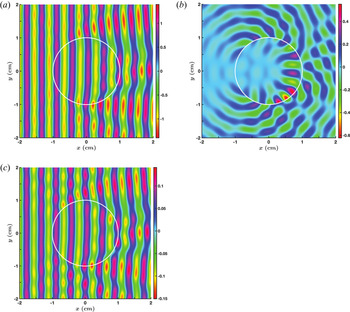
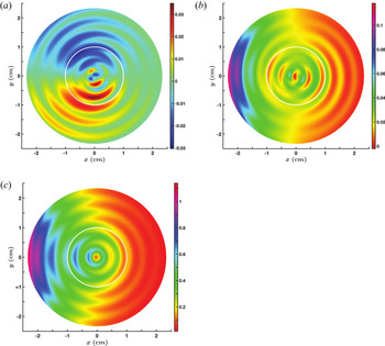
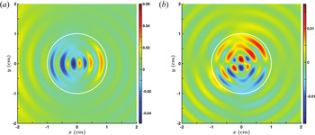
The numerical solutions resulting from the analytical theory support this simple reasoning. Figure 5 shows the real part of the Cartesian components of the total electric field $\boldsymbol {E}_T = \boldsymbol {E}_I + \boldsymbol {E}_S + \boldsymbol {E}_F$ normalized to $| \mathcal {E}_0 |$. Figures 5(a) and 5(c) show the planar wavefronts that are slightly distorted by the presence of the filament. As mentioned previously, this is to be expected because the properties of the slow wave inside and outside the filament are approximately the same. Furthermore, because the incoming slow wave has $P_{0y} = 0$ while $( P_{0 x}, \, P_{0 y} ) \ne 0$, the planar wave fronts exist for $\textrm {Re} ( E_{Tx} )$ and $\textrm {Re} ( E_{Tz} )$ only. From (9.5), for the incident wave, the maximum amplitudes of $\textrm {Re} ( \mathbb {E}_{0x} )$ and $\textrm {Re} ( \mathbb {E}_{0z} )$ are $0.995$ and $0.098$, respectively.

Figure 5.

Contours of the Cartesian components of the total electric field $\boldsymbol {E}_T$ in the $x$–$y$ plane, when the incident plane wave is a slow LH wave; $\boldsymbol {E}_T = \boldsymbol {E}_I + \boldsymbol {E}_S + \boldsymbol {E}_F$ is the vector sum of the incident and scattered fields and fields inside the filament. The wave is incident from the left, and the cross-sectional outline of the cylindrical filament (radius $a = 1$ cm) is shown in white. The plasma and wave parameters are given in table 1. (a) Contours of $\textrm {Re} ( E_{T x} )$. (b) Contours of $\textrm {Re} ( E_{T y} )$. (c) Contours of $\textrm {Re} ( E_{T z} )$ .

The maximum amplitudes of $\textrm {Re} ( E_{Tx} )$ and $\textrm {Re} ( E_{Tz} )$ are approximately the same as shown in figures 5(a) and 5(c). The wavefronts in figure 5(b) for the $y$-component of the electric field are, definitely, not planar. This is an effect of the evanescent fast wave, generated inside the filament, which retains some spatial aspects of the cylindrical geometry. The figure shows an enhancement of the electric field near the boundary of the filament in agreement with the discussion in the previous paragraph. In addition, the maximum value of $\textrm {Re} ( E_{Ty} )$ is much larger than the maximum value of $\textrm {Re} ( \mathbb {E}_{0y} )$: the larger value of $\textrm {Re} ( E_{k \phi F}^{f} )$ (table 1) being the contributing factor. The enhanced fields of the evanescent fast wave near the boundary generate a propagating fast wave in the background plasma.

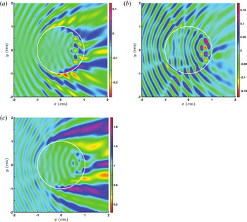
The coupling to the fast wave has consequences on the flow of wave energy. Figure 6 shows the three Cartesian components of the Poynting vector $\boldsymbol {P}$ for the complete set of electromagnetic fields. The power flow in the $y$-direction inside and outside the filament is a direct result of coupling to the fast mode since only the fast wave inside the filament has a non-zero power flow in the $y$-direction. Figures 6(a) and 6(c) show the diffraction pattern due to scattering in the wake of the filament.

Figure 6.

Contours of the three Cartesian components of the Poynting vector associated with the fields in figure 5. (a) Contours of $P_x$. (b) Contours of $P_y$. (c) Contours of $P_z$.

9.2.2. Scattering of a fast LH plane wave

The scattering is interestingly different if, instead of the slow LH wave, the incident plane wave is the fast LH wave. From table 1, we note that $\lambda _{0x} / a = 9.25 \gg 1$, that is, the wavelength of the incident wave is much longer than the radial dimension of the filament. Consequently, the electric field of the incident plane wave will have a very small spatial variation across the filament. As the fast wave is evanescent inside the filament and its polarization, especially the $z$-component, is quite different from the incident wave, we do not expect a coupling between the fast waves inside and outside the filament. The boundary conditions (6.1)–(6.4) can only be satisfied if we account for the slow wave inside the filament. Given that $\lambda _{\rho S}^{f} / a \approx 0.5$, we expect two radial wavelengths of the slow wave to fit inside the filament. The contribution to (5.5) from the propagating slow wave depends on $\textrm {J}_m ( k_{\rho S}^{f} \rho )$ and $\textrm {J}_m' ( k_{\rho S}^{f} \rho )$ with $k_{\rho S}^{f}$ being real and $0 \le \rho \le a$. We find that only for $m=0,\ 1,\ \textrm {and}\ 2$, do the Bessel functions have two ‘wavelengths’ inside the filament (figure 7). With this limitation on the azimuthal mode number, we expect the wave fields inside the filament to be radially structured having a wavelength of $0.47$ cm, and an azimuthal variation corresponding to $m = 1 \ \textrm {and} \ 2$.

Figure 7.

Variation of the Bessel functions (and derivatives) as a function of $\rho$ inside the filament: (a) $\textrm {J}_m$ as a function of $\rho$ for $m = 0,\ 1,\ \textrm {and} \ 2$; (b) $\textrm {J}_m'$ as a function of $\rho$ for $m = 0,\ 1,\ \textrm {and} \ 2$. The argument of the Bessel function is $k_{\rho S}^{f} \rho$, with $k_{\rho S}^{f} = \omega n_{\rho S}^{f} / c \approx 13.403$ cm$^{-1}$ being the $\hat {\boldsymbol {\rho }}$ component of the LH fast wave vector inside the filament. The parameters are as in table 1.

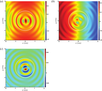
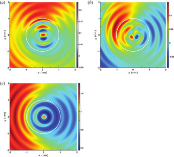
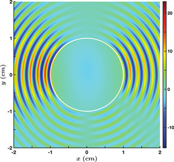
Figures 8 and 9 show the scattering of the incident fast wave by the filament. The generation of the slow wave inside the filament is evident. The radial variation is as expected as are the $m=1\ \textrm {and} \ 2$ azimuthal structures.

Figure 8.

Contours of the Cartesian components of $\boldsymbol {E}_T$ when a fast LH wave is incident from the left. The parameters are the same as for figure 5. (a) Contours of $\textrm {Re} ( E_{T x} )$. (b) Contours of $\textrm {Re} ( E_{T y} )$. (c) Contours of $\textrm {Re} ( E_{T z} )$.

Figure 9.

Contours of the three Cartesian components of the Poynting vector associated with the fields in figure 8. (a) Contours of $P_x$. (b) Contours of $P_y$. (c) Contours of $P_z$.

The physics of the generation of the slow wave inside the filament is simple. The electric field of the incident plane wave induces dipole oscillations at the interface of the filament. These oscillations, in turn, generate a propagating wave inside the filament that is consistent with the geometry and with the electromagnetic boundary conditions. The filament behaves like an antenna and excites cylindrical slow waves in the background plasma. While the incident plane wave has $P_{0y} = 0$, the scattering leads to Poynting flux in the $y$-direction. Unlike the case of an incident slow wave where $P_{0y} \ne 0$ due to the presence of an evanescent fast wave inside the filament, here it is the propagating slow wave inside the filament that leads to $P_{0y} \ne 0$. The incident plane wave has $k_{0y} = 0$. The cylindrical wavefronts of the slow wave lead to $k_{yS}^{f} \ne 0$ which, in turn, leads to $P_{y} \ne 0$. 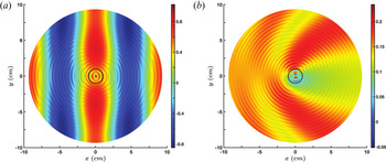It is worth noting that, over the spatial scales shown in the figures, there is no obvious presence of the incident plane wave, its wavelength being over $9$ cm. In figure 10(a), we display results over an extended range. The planar phase front of the incident wave is clearly discernable, as is the uniformity of the incident wave field over the filament cross-section. Figure 10(b) shows that the filament affects the spatial variation of power flow over a much wider region compared with its cross-section.

Figure 10.

Same as figures 8(a) and 9(a), respectively, except that the display is over a wider region of space. The fast wave with its wavelength of $9.25$ cm is clearly discernable, as is the effect of the slow wave on the power flow in the $x$-direction. The cross-section of the filament is in black. (a) Contours of $\textrm {Re} ( E_{T x} )$. (b) Contours of $P_x$.

9.2.3. Scattering of a fast LH plane wave by a filament with smaller radius

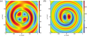
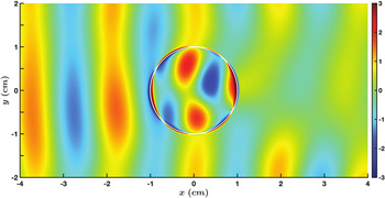
If the radius of the filament is smaller than the radial wavelength of the slow wave, the electric field structure inside the filament changes. Even so, the effect on the surrounding plasma is the same as in figure 8. The real part of the $x$ and $z$ components of the total electric field in the presence of a filament of radius $a = 0.4$ cm are shown in figure 11. From the radiation patterns we note that the filament behaves like a dipole antenna (Lai et al. Reference Lai, Zheng, Zhang and Chan2010). Inside the filament, the $m = 1$ pattern is seen in figure 11(b) for the $\textrm {Re} ( E_{Tz} )$; the radial structure follows from the Bessel function of order 1, $\textrm {J}_1 ( k_{\rho S}^{f} \rho )$, with $0 \ge \rho \ge 0.4$ cm (see figure 7a). The azimuthal variation of $\textrm {Re} ( E_{Tx} )$ in figure 11(a) has the structure of a $m = 2$ mode: the $x$-component of the field having an extra $\sin ( \phi )$ multiplier when converting from a cylindrical coordinate system to the Cartesian system.

Figure 11.

Results for the same conditions and parameters as in figure 8 except that $a = 0.4$ cm. The wavelength of the incoming fast LH wave is $9.25$ cm (see figure 10a). (a) Contours of $\textrm {Re} ( E_{T x} )$. (b) Contours of $\textrm {Re} ( E_{T z} )$.

If we reduce the radius of the filament to $0.25$ cm, the radiation patterns are similar to those shown in figure 11. This leads to a compelling observation. Even if the wavelength of the incident RF wave is much longer than the radial extent of the filament, in this case the ratio is greater than 10, the scattered fields are significantly modified by the presence of the filament. Consequently, even if the spatial scale length of the turbulence is much shorter than the RF wavelength and the density variation is small, the effect of turbulence on RF waves cannot be neglected.

9.3. Scattering of an evanescent LH wave

So far we have studied the scattering of waves that propagate in the background plasma. However, evanescent waves can exist in the low-density plasma in the vicinity of an RF source. This is evident from the dispersion relation in figure 2. For scattering of an evanescent wave, we interchange the plasma parameters for the background and the filament in table 1. In this case, the filament density $2.25 \times 10^{19}$ m$^{-3}$ is larger than the background density $2 \times 10^{19}$ m$^{-3}$. An incident fast wave is an evanescent mode for which the electric field amplitude decays with distance. Inside the filament, both the slow and fast waves are propagating modes with $\lambda _{\rho S}^{f} / a < 1$ and $\lambda _{\rho F}^{f} / a \gg 1$ for $a = 1$ cm. From our discussions, it is reasonable to expect that an incident (evanescent) fast wave will excite the slow wave inside the filament; essentially no power being coupled to the fast mode as its wave characteristics do not match those of the incident wave. Indeed, as shown in figures 12 and 13, that is exactly what we observe in the simulations. The excitation of the cylindrical slow wave inside the filament generates a cylindrical slow wave in the surrounding plasma. The filament, in effect, is instrumental in coupling power from an evanescent wave to a propagating wave in the background plasma. The incident wave has $P_{0x} = 0$. The propagating wave excited by the filament has a $P_x \ne 0$ which carries some of the incident power in towards the core plasma.

Figure 12.

Contours of the Cartesian components of $\boldsymbol {E}_T$ when an evanescent LH fast wave, incident from the left, is scattered by a filament with $a = 1$ cm. The parameters are the same as in table 1 except that the background and filament densities are interchanged, that is, $n_e^{b} = 2 \times 10^{19}$ m$^{-3}$ and $n_e^{f} = 2.25 \times 10^{19}$ m$^{-3}$. (a) Contours of $\textrm {Re} ( E_{T x} )$. (b) Contours of $\textrm {Re} ( E_{T y} )$. (c) Contours of $\textrm {Re} ( E_{T z} )$.

Figure 13.

Contours of the three Cartesian components of the Poynting vector associated with the fields in figure 12. (a) Contours of $P_x$. (b) Contours of $P_y$. (c) Contours of $P_z$.

9.4. Scattering when the density differential is large

An analysis of experimental data shows that the density fluctuations in the edge region can be significantly larger than the background density (Zweben et al. Reference Zweben, Maqueda, Terry, Munsat, Myra, D'Ippolito, Russell, Krommes, LeBlanc and Stoltzfus-Dueck2006, Reference Zweben, Boedo, Grulke, Hidalgo, LaBombard, Maqueda, Scarin and Terry2007). We consider such a case and show that the physics of RF scattering follows along the same path discussed above. In the following, we assume that the electron density inside the filament is $4 \times 10^{19}$ m$^{-3}$, while the background density is $2 \times 10^{19}$ m$^{-3}$. From figure 2, we note that both the slow and fast LH waves are propagating modes inside the filament, while only the slow LH wave propagates in the background plasma. The dispersion equation (4.10) yields

(9.7a,b)\begin{gather} \varLambda_{\rho S}^{b} = \left( 0.47,\, 0 \right)\, \textrm{cm}, \quad \varLambda_{\rho F}^{b} = \left( 0,\, -12.5 \right)\, \textrm{cm}, \end{gather}

(9.8a,b)\begin{gather} \varLambda_{\rho S}^{f} = \left( 0.358,\, 0 \right)\, \textrm{cm}, \quad \varLambda_{\rho F}^{f} = \left( 2.165,\, 0 \right)\, \textrm{cm}. \end{gather}

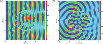
If the incoming wave is the slow LH wave, then $\lambda _{\rho S}^{b}$ is comparable to $\lambda _{\rho S}^{f}$ but much shorter than $\lambda _{\rho F}^{f}$. This situation is similar to that discussed in § 9.2.1. Figures 14(a) and 14(b) show the contours of $\textrm {Re} ( E_{Tx} )$ and $\textrm {Re}( E_{Ty} )$, respectively. These results bear remarkable resemblance to the corresponding plots in figure 5 even though the parameters are very different.

Figure 14.

Contours of Re$( E_{Tx} )$ and Re$( E_{Ty} )$, respectively, when a propagating slow LH wave is incident from the left. Here, $a = 1$ cm, $n_e^{b} = 2 \times 10^{19}$ m$^{-3}$, $n_e^{f} = 4 \times 10^{19}$ m$^{-3}$, $B_0 = 4.5$ T, $\nu = 4.6$ GHz and $n_z = 2$. (a) Contours of $\textrm {Re} ( E_{T x} )$. (b) Contours of $\textrm {Re} ( E_{T y} )$.

If the incoming LH wave is the evanescent fast wave, we expect both the fast and slow LH waves to be excited inside the filament. However, from (9.8a,b), for $a = 1$ cm, $\lambda _{\rho F}^{f} / a > 1$ while $\lambda _{\rho S}^{f} / a < 1$, so that the field structure inside the filament will be dominated by the slow wave. This, in turn, will couple power to the slow propagating wave in the background plasma with a radial wavelength of $0.47$ cm. The contours of Re$( E_{Tx} )$ and Re$( E_{Ty} )$ in figures 15(a) and 15(b), respectively, clearly illustrate this scattering process. Whereas the incident wave has no power flow in the $x$-direction, the scattered wave carries power in this direction. The similarity with figures 12(a) and 12(b) indicates that the physics of the scattering process is analogous to that in § 9.3.

Figure 15.

Contours of Re$( E_{Tx} )$ and Re$( E_{Ty} )$, respectively, when an evanescent fast plane LH wave is incident from the left. The plasma and wave parameters are as for figure 14. (a) Contours of $\textrm {Re} ( E_{T x} )$. (b) Contours of $\textrm {Re} ( E_{T y} )$.

9.5. Scattering of LH waves with a different frequency

For comparison, we assume that all the parameters are the same as in § 9.4 except for the wave frequency. For $\nu = 2.45$ GHz, we find that

(9.9a,b)\begin{gather} \varLambda_{\rho S}^{b} = \left( 0.451,\, 0 \right)\, \textrm{cm}, \quad \varLambda_{\rho F}^{b} = \left( 4.789,\, 0 \right)\, \textrm{cm}, \end{gather}

(9.10a,b)\begin{gather} \varLambda_{\rho S}^{f} = \left( 0.333,\, 0 \right)\, \textrm{cm}, \quad \varLambda_{\rho F}^{f} = \left( 1.989,\, 0 \right)\, \textrm{cm}. \end{gather}

The main difference, when comparing with (9.7a,b) and (9.8a,b), is that the fast wave is a propagating wave at this lower frequency (figure 4). Consequently, if the incident wave is the slow LH wave, we do not expect much difference in the scattering due to the frequency change. We find that the results are similar to those shown in figures 14(a) and 14(b). When the incident wave is the fast LH wave, we can deduce the effect of the filament from these two conditions: $\lambda _{\rho F}^{b}/ a > 4$ and $\lambda _{\rho F}^{f}/ a \approx 2$. The first condition implies that the electric field of the incoming wave is essentially uniform over the cross-section of the filament. The second conditions implies that it will be difficult to set up a fast wave eigenmode inside the filament. As $\lambda _{\rho S}^{f} / a < 1$, the incident wave will excite the short-wavelength slow wave inside the filament that couples power to the scattered slow wave outside the filament. It follows that the total field should look essentially the same as in figures 15(a) and 15(b). Not surprisingly, numerical simulations support this intuitive argument. The details of the cylindrical wave patterns are different between the two frequencies, but the global structure of the scattering is essentially the same.

10. Scattering of helicon waves

The scattering of LH waves provides a useful base for studying the scattering of lower-frequency waves. Toward this end, we first consider the scattering of helicon waves and, in the subsequent section, scattering of IC waves.

Helicon waves exist in a frequency range that is below the LH frequency, but well above the IC frequency (Stix Reference Stix1992; Bers Reference Bers2016). It is believed that helicon waves can efficiently induce plasma currents in toroidal fusion devices, and experiments in DIII-D are being planned to test this premise (Pinsker et al. Reference Pinsker, Prater, Moeller, de Grassie, Petty, Porkolab, Anderson, Garofalo, Lau and Nagy2018). The roots of the cold plasma dispersion relation (4.10) are plotted in figure 16 for DIII-D type parameters that will be used in our study. The slow helicon wave has a resonance, the LH resonance, at $n_e^{LHR} \approx 2.25 \times 10^{19}$ m$^{-3}$. For electron densities higher than $n_e^{LHR}$, the slow wave is evanescent. The fast helicon wave, experimentally favoured as it can access high plasma densities, has a cutoff which is a function of $n_z$ (Bers Reference Bers2016). The density at which the cutoff occurs can be deduced from (4.10). For our choice of parameters, the cutoff density is $n_{e}^{C} \approx 3.5 \times 10^{18}$ m$^{-3}$ (figure 16).

Figure 16.

Variation of the cold plasma dispersion roots for helicon waves, obtained from (4.10), as a function of the electron density. SW and FW indicate the slow and fast waves, respectively, and LHR marks the density location of the LH resonance. The parameters are $B_0 = 1.4$ T, $\nu = 476$ MHz and $n_z = 4$.

The density range covered in figure 16 can be divided into four distinct regions. In each region the wave physics and wave scattering are different. Even though we have carried out detailed numerical simulations for parameters corresponding to a specific region, the narrative follows the following rule. For situations that bear similarities to LH scattering, we discuss the physics without showing any figures. Otherwise, we supplement the discussion with graphs. In all cases we assume that the incident plane wave is the fast helicon wave.

Case 1: $n_e \le n_e^{C}$ For densities below $n_e^{C}$, the incident fast wave is evanescent. The propagating slow wave has $\lambda _{\rho S}^{b,f} \gtrapprox 0.424$ cm in the density range $[ 10^{17}, 3.5 \times 10^{18} ]$ m$^{-3}$. In the filament and the background plasma, the slow wave will be excited by coupling of waves at the boundary. The wave field structure inside the filament will depend on the argument $2 {\rm \pi}\rho / \lambda _{\rho S}^{f}$ of the Bessel functions. If $a / \lambda _{\rho S}^{f} > 1$, the field patterns will be similar to those in figures 8 and 12, otherwise the fields will be of the form shown in figure 11. In either case, there will be an outflow of power due to the scattered slow cylindrical waves propagating in the background plasma.

Case 2: $n_e^{C} < n_e < n_e^{LHR}$ For these densities the fast and the slow helicon waves are propagating modes with $\lambda _{\rho F}^{b,f} > 2.53$ cm while $0 < \lambda _{rho S}^{b,f} \lessapprox 0.424$ cm. It should be noted that, in the vicinity of the LH resonance, the cold plasma model for the dispersion relation breaks down: thermal effects need to be included in the wave description (Bers Reference Bers2016). For filaments with $a \lessapprox 1$ cm, $\lambda _{\rho F}^{b,f} > a$ while for the slow waves $\lambda _{\rho S}^{b,f} \lessapprox a$. The electric fields inside the filament are primarily those of the slow wave, and the total fields are similar to those in figures 8 and 10. The number of cylindrical wavelengths inside the filament depends on the density. For example, for $n_e^{f} = 1.5 \times 10^{19}$ m$^{-3}$, $1/\lambda _{\rho S}^{f} \approx 7.74$ cm$^{-1}$, and the argument of the Bessel functions is $\approx 48.63 a$. For $a = 1$ cm, the number of oscillations of the Bessel functions of low order is approximately seven. The results from full numerical simulations confirm this estimate.

Case 3: densities in the vicinity of the LH resonance If the background density is between $n_e^{C}$ and $n_e^{LHR}$ and the density inside the filament is $> n_e^{LHR}$, then the fast and slow waves are propagating modes in the background plasma, while only the fast wave is a propagating mode inside the filament, with the slow wave being an evanescent mode. For an incident fast wave, we do not expect any slow cylindrical waves being generated inside the filament. However, the evanescent wave can still couple power to the propagating slow wave outside the filament. Consider the following example where the background plasma density is $10^{19}$ m$^{-3}$ and the density inside the filament is $3 \times 10^{19}$ m$^{-3}$. Then,

(10.1a,b)$$\begin{gather} \varLambda_{\rho F}^{b} = \left( 6.02, \, 0 \right) \, \textrm{cm}, \quad \varLambda_{\rho S}^{b} = \left( 0.204, \, 0 \right) \, \textrm{cm}, \end{gather}$$

(10.2a,b)$$\begin{gather}\varLambda_{\rho F}^{f} = \left( 1.88, \, 0 \right) \, \textrm{cm}, \quad \varLambda_{\rho S}^{f} = \left( 0, \, -0.09 \right) \, \textrm{cm}. \end{gather}$$

Inside the filament, the evanescent slow mode is localized close to the surface since the real (imaginary) part of even order (odd order) Bessel functions for imaginary $\varLambda _{\rho S}^{f}$ in (10.2a,b) peak near $\rho \approx a$. For $a = 1$ cm, the wavelength of the fast wave, inside and outside the filament, is longer than the radius of the filament. Thus, the fast wave fields inside the filament will have very weak spatial variation. These expectations, based on the previous results for LH waves, are borne out by numerical simulations. The contours of Re$( E_{Tx} )$ in figure 17 show the uniformity of fields inside the filament, the narrow region of enhanced fields near the boundary, and the cylindrical slow wave propagating away from the filament. The scattered slow wave leads to side scattering of the incoming fast wave and affects the power flow into the core.

Figure 17.

Contours of Re$( E_{Tx} )$ in the $x$–$y$ plane for the scattering of a fast helicon wave when the plasma density is greater than the cutoff density of the fast wave. The parameters are the same as in figure 16 along with $a = 1$ cm, $n_e^{b} = 10^{19}$ m$^{-3}$ and $n_e^{f} = 3 \times 10^{19}$ m$^{-3}$.

Case 4: $n_e > n_e^{LHR}$  The only propagating mode is the fast wave with $\lambda _{\rho F}^{b,f} < 2.53$ cm. The electric field due to the evanescent slow wave will be localized near the surface of the filament given by the maxima of the Bessel functions and the Hankel functions of the first kind for complex argument. We expect that there will be some resemblance to the results shown in figure 5. For illustrative purposes, we assume the background plasma density and the density inside the filament to be $3 \times 10^{19}$ m$^{-3}$ and $5 \times 10^{19}$ m$^{-3}$, respectively. The corresponding (complex) wavelengths are

(10.3a,b)$$\begin{gather} \varLambda_{\rho F}^{b} = \left( 1.88, \, 0 \right) \, \textrm{cm}, \quad \varLambda_{\rho S}^{b} = \left( 0, \, -0.09 \right) \, \textrm{cm}, \end{gather}$$

(10.4a,b)$$\begin{gather}\varLambda_{\rho F}^{f} = \left( 1.12, \; 0 \right) \, \textrm{cm}, \quad \varLambda_{\rho S}^{f} = \left( 0, \, -0.14 \right) \, \textrm{cm}. \end{gather}$$

Figure 18 shows contours of Re$( E_{Tx} )$ with $a = 1$ cm, comparable to the wavelength of the fast wave. The planar phase front of the incoming wave gets distorted by the filament, with a shadow in its wake. The presence of large-amplitude slow wave fields near the boundary is evident even though we have suppressed the maximum amplitude in order to display the rest of the field pattern.

Figure 18.

Contours of Re$( E_{Tx} )$ in the $x$–$y$ plane for the scattering of a fast helicon wave when the plasma density is greater than the density at which the LH resonance occurs. The parameters are the same as in figure 16 along with $a = 1$ cm, $n_e^{b} = 3 \times 10^{19}$ m$^{-3}$ and $n_e^{f} = 5 \times 10^{19}$ m$^{-3}$. The maximum amplitude of the evanescent slow wave field at the filament boundary has been truncated so as to enhance the contrast of the field in other regions.

11. Scattering of IC waves

A preferred means of heating toroidal plasma is by RF waves in the IC range of frequencies; in particular, the fast Alfvén wave (FAW). The cold plasma dispersion characteristics of these waves are plotted in figure 19 in the density range appropriate for the edge plasma in a SPARC-like, high-magnetic-field tokamak (Lin, Wright & Wukitch Reference Lin, Wright and Wukitch2020). Just like helicon waves, the slow IC wave propagates for densities less than $n_{e}^{LHR} \approx 4.27 \times 10^{17}$ m$^{-3}$ (figure 19). For larger densities, the slow wave is evanescent. The fast wave is evanescent until its cutoff density $n_{e}^{C} \approx 2.16 \times 10^{19}$ m$^{-3}$, after which it becomes a propagating wave. Unlike helicon waves, the slow and fast waves propagate in distinctly different density regimes. In the discussion that follows, we assume that the incoming plane wave is the FAW.

Figure 19.

The cold plasma dispersion roots in the IC range of frequencies, obtained from (4.10), as a function of the electron density. SW and FW indicate the slow and fast Alfvén waves, respectively, and LHR marks the density location of the LHresonance. The ordinate scale on the left is for the slow wave and that on the right is for the fast wave. The parameters are $B_0 = 9.3$ T, $\nu = 120$ MHz and $n_z = 6$.

From the result for helicon waves, we can deduce that, for densities below $n_e^{LHR}$, the FAW will couple to the slow wave inside the filament; thereby exciting slow cylindrical waves in the background plasma. In the density range $[ n_e^{LHR}, \; n_e^{C} ]$ both wave modes are evanescent. The Bessel functions of imaginary argument, for the two modes inside the filament, peak near $\rho \approx a$. The Hankel functions of the first kind of an imaginary argument ensure that the scattered wave fields decay away for $\rho > a$. Consequently, the wave fields will peak in the vicinity of the boundary of the filament.

For densities greater than $n_e^{C}$, the FAW is a long-wavelength mode with $a/ \lambda _{\rho F}^{b,f} \ll 1$ for any reasonable value of $a$. Accordingly, we do not expect any wave-like features, associated with the slow wave, inside the filament. The electromagnetic fields will essentially be uniform over the cross-section except in the vicinity of the boundary where the fields have to match on to the incident and scattered fields. In this density regime, there is no analogous situation for LH and helicon waves. As an example, consider a filament with density $7 \times 10^{19}$ m$^{-3}$ surrounded by a plasma with density $4 \times 10^{19}$ m$^{-3}$. The corresponding wavelengths are

(11.1a,b)$$\begin{gather} \varLambda_{\rho F}^{b} = \left( 30.6, \, 0 \right) \, \textrm{cm}, \quad \varLambda_{\rho S}^{b} = \left( 0, \, -0.45 \right) \, \textrm{cm}, \end{gather}$$

(11.2a,b)$$\begin{gather}\varLambda_{\rho F}^{f} = \left( 18.2, \, 0 \right) \, \textrm{cm}, \quad \varLambda_{\rho S}^{f} = \left( 0, \, -0.36 \right) \, \textrm{cm}. \end{gather}$$

For a FAW incident on a filament with $a = 1$ cm, $a/\lambda _{\rho F}^{b,f} \ll 1$ and the fields inside the filament can be expected to be uniform over the cross-section. As the FAW is a propagating mode inside the filament, it cannot screen out the fields of the incident FAW. Thus, in the vicinity of $\rho \approx 0$ we expect the field amplitudes to be non-zero. In (5.5) for wave fields inside the filament, only the $m = \pm 1$ azimuthal modes, corresponding to $\textrm {J}'_{\pm 1} ( k_{\rho F}^{f} a )$, are non-zero. The $m = \pm 1$ feature is evident in the result from numerical simulations shown in figure 20(a).

Figure 20.

Contours of (a) Re$( E_{Tx} )$ and (b) $P_z$ when a FAW, incident from the left, scatters off a filament with $a = 1$ cm. The parameters are, $B_0 = 9.3$ T, $\nu = 120$ MHz, $n_z = 6$, $n_e^{b} = 4 \times 10^{19}$ m$^{-3}$ and $n_e^{f} = 7 \times 10^{19}$ m$^{-3}$. (a) Contours of $\textrm {Re} ( E_{T x} )$. (b) Contours of $P_z$.

For helicon waves, the presence of a similar feature is discernable in figure 17. The large-amplitude electric fields inside the filament are responsible for an enhanced flow of Poynting flux in the $z$-direction as shown in figure 20(b). For comparison, the Poynting flux in $z$-direction for the incoming FAW is $0.88$. Intuitively, one would expect the filament to play an insignificant role in the scattering process because the wavelength of the incoming wave is much larger than the radial extent of the filament. However, the results show otherwise. A fraction of the incident wave power will be converted to flow down the axis of the filament along the magnetic field line.

12. Maxwell stress tensor: radial force on a filament

In 1905, Poynting studied the radiation pressure of light at an interface separating two different dielectric media described by scalar permittivities (Poynting Reference Poynting1905; Loudon & Baxter Reference Loudon and Baxter2012). He came to an interesting conclusion, which he followed up with supporting experiments. Poynting stated the following:

The ‘pull’ and ‘push’ are defined with respect to the direction of propagation of the incident light: the pull being opposite to this direction and the push being along this direction. Thus, according to Poynting, the incident light will pull the glass along the outward pointing normal to the interface. Poynting's research was a contributing factor to the Minkowski–Abraham controversy regarding the definition of electromagnetic momentum within dielectric media (Loudon & Baxter Reference Loudon and Baxter2012). The permittivity of a magnetized plasma is a tensor rather than a scalar. Consequently, as we have already noted, not only is there a wider variety of waves that can exist in a plasma, compared with a scalar dielectric, but also the filament induces coupling between these different waves. Following the Maxwell stress tensor formulation in § 7, we examine the radiation force on a filament by different plasma waves, discussed in §§ 9, 10 and 11, and compare with Poynting's observations.

In order to have a meaningful quantitative measure, we calculate the acceleration of a representative filament due to the radiation force. From (7.14) and (8.5), the force on a filament per unit incident power flux is defined as

(12.1) \begin{equation} \left( \begin{array}{@{}c@{}}{\tilde{\mathcal{F}}}_x \\ {\tilde{\mathcal{F}}}_y \end{array} \right) = \frac{1}{S_I} \left( \begin{array}{@{}c@{}}{\mathcal{F}}_x \\ {\mathcal{F}}_y \end{array} \right) = \frac{a}{c} \, \int_{0}^{2 {\rm \pi}} \, \textrm{d}\phi \left( \begin{array}{@{}c@{}} \cos \phi \\ \sin \phi \end{array} \right) F_{\rho} \left( \phi \right) \quad \frac{\textrm{N m}^{{-}1}}{\textrm{W m}^{{-}2}}, \end{equation}

where we have assumed that the filament has an axial length of $1$ m. It turns out that, for all the scattering events we have studied, ${\mathcal {F}}_y = 0$. Various attempts at proving this result analytically have not been successful; so we leave this as an exercise for the future. For ${\mathcal {F}}_x < 0$ the force is towards the RF source (‘pull’), while for ${\mathcal {F}}_x > 0$ the force is away from the source (‘push’). The acceleration of the filament in the $x$-direction is

(12.2)\begin{equation} {\mathfrak a}_x = \frac{\tilde{\mathcal{F}}_x}{\mathfrak m}, \end{equation}

where ${\mathfrak m}$ is the mass of the filament. As in the scattering studies, a filament will have deuterons and electrons only, so that ${\mathfrak m} = 1.05 \times 10^{-26} \, a^{2} \, n_e^{f}$ kg. Unless stated otherwise, in all the subsequent calculations we assume that $a = 1$ cm, and the input RF power flux is $1$ kW m$^{-2}$. The primary plasma parameters, magnetic field, wave frequency and $n_z$, for the LH, helicon and IC waves are as in figures 2 $( S_1,\, F_1 )$, 16 and 19, respectively.

12.1. Radiation force due to LH waves: variation with filament radius

In §§ 9.2.1 and 9.2.2 we discussed the scattering of slow and fast LH waves, respectively, by a filament. The radial force on the filament $F_\rho$, given in (8.5), is plotted as a function of the azimuthal angle $\phi$ for the slow wave in figure 21(a) and for the fast wave in figure 21(b).

Figure 21.

The normalized stress force as a function of the azimuthal angle. The parameters for the slow and fast LH waves are the same as for figures 5 and 8, respectively. (a) Incident plane wave is the slow LH wave. (b) Incident plane wave is the fast LH wave.

The difference between the two results can be traced to the corresponding field plots in figures 5 and 8. For the slow wave, the fields at the surface of the filament have a wide range of variations in the azimuthal direction. The incoming wave is distorted around the surface of the filament due to geometrical mismatch between the planar wave and the cylindrical filament. For the fast wave the variation is almost sinusoidal as cylindrical waves generated within the filament dominate the field pattern. The integration of these profiles over $\phi$ yields the force on the filament per unit power flow of the incident wave,

(12.3a,b)\begin{equation} \left. \tilde{\mathcal{F}}_x \right|_{S,LH} = 4.23 \ \frac{\textrm{nN m}^{{-}1}}{\textrm{kW m}^{{-}2}}, \quad \left. \tilde{\mathcal{F}}_x \right|_{F,LH} ={-}56.13 \ \frac{\textrm{nN m}^{{-}1}}{\textrm{kW m}^{{-}2}}, \end{equation}

for the slow and fast waves, respectively. The slow wave is ‘pushing’ away the filament while the fast wave is ‘pulling’ it in towards the RF source. The filament density assumed in the simulations $n_e^{f} = 2 \times 10^{19}$ m$^{-3}$ yields ${\mathfrak m} = 2.1 \times 10^{-11}$ kg. The corresponding accelerations are

(12.4a,b)\begin{equation} \left.{\mathfrak a}_x \right|_{S,LH} = 2.0 \times 10^{2} \, \textrm{m}\,\textrm{s}^{{-}2}, \quad \left.{\mathfrak a}_x \right|_{F,LH} ={-}2.7 \times 10^{3} \, \textrm{m}\,\textrm{s}^{{-}2}. \end{equation}

Even though the dynamics of a filament through a background plasma requires more physics, the acceleration gives a measure of the effect of RF waves on the filament. Clearly, the direction of the force will play a role in the motion of the filament.

The scattering by a filament of smaller radius, $a < 1$ cm, was discussed in §9.2.3. For two different radii, the acceleration due to the slow and fast LH waves is

(12.5)\begin{equation} \left. \begin{aligned} \textrm{for} \, a & = 0.4 \, \textrm{cm}: \quad \left.{\mathfrak a}_x \right|_{S,LH} = 4.7 \times 10^{2} \, \textrm{m}\,\textrm{s}^{{-}2}, \quad \left. {\mathfrak a}_x \right|_{F,LH} ={-}5.5 \times 10^{3} \, \textrm{m}\,\textrm{s}^{{-}2}, \\ \textrm{for} \ a & = 0.25 \, \textrm{cm}: \quad \left.{\mathfrak a}_x \right|_{S,LH} = 7.5 \times 10^{2} \, \textrm{m}\,\textrm{s}^{{-}2}, \quad \left.{\mathfrak a}_x \right|_{F,LH} ={-}1.3 \times 10^{4} \, \textrm{m}\, \textrm{s}^{{-}2}. \end{aligned} \right\} \end{equation}

Comparing with (12.4a,b), we note that the acceleration increases as the radial dimension of the filament decreases while preserving the direction of the force.

12.2. Radiation force due to propagating slow waves: the push–pull effect

In this subsection, we compare the radiation force due to the slow wave on a filament with density $n_{e}^{f} < n_{e}^{b}$ with that when $n_{e}^{f} > n_{e}^{b}$, for the LH, helicon and IC waves. For LH waves the slow wave is preferred in experiments, whereas for helicon and IC waves it is the fast wave. Nonetheless, we consider the slow wave in all three frequency ranges to determine whether there is any dependence of the radiation force on frequency.

12.2.1. Lower hybrid waves

In § 12.1, the densities were such that $n_{e}^{f} < n_{e}^{b}$. If we only change the filament density to $n_{e}^{f} = 2.5 \times 10^{19}\, \textrm {m}^{-3}$, then $n_{e}^{f} > n_{e}^{b}$ and the acceleration due to the slow wave is

(12.6)\begin{equation} \left.{\mathfrak a}_x \right|_{S,LH} ={-}1.6 \times 10^{2} \, \textrm{m}\,\textrm{s}^{{-}2}. \end{equation}

Comparing with the results in (12.4a,b), there is a change in sign of the force. This reversal of the ‘push–pull’ effect was initially recognized by Poynting (Loudon & Baxter Reference Loudon and Baxter2012). In his formulation, for normal incidence on a planar surface separating two different dielectric media, the direction of the force depended on the relative refractive indices of the media. For light incident from a region of lower refractive index, the force was towards the region of lower refractive index. For light incident from a region of higher refractive index, the force was still towards the region of lower refractive index. While the scattering from a filament is different from a planar interface, the reversal in sign is intriguing. For the results in (12.4a,b), the wave is propagating from a region of higher refractive index (higher plasma density) to a filament with lower refractive index (lower plasma density). For (12.6) the incident wave is in a region with lower refractive index. The direction of the radiation force due to an incident slow wave follows Poynting's observations. The force due to the slow wave is such that higher-density (relative to the background density) filaments are pulled in towards the RF source, while the lower-density filaments are pushed away. The effect of the radiation force is to create a density inversion in the vicinity of the source.

12.2.2. Helicon waves

For helicon waves, the slow mode is a propagating wave for $n_e^{b,f} < n_e^{LHR} \approx 2.25 \times 10^{19}$ m$^{-3}$ (figure 16). For an ambient density $n_e^{b} = 5 \times 10^{17}$ m$^{-3}$, assume two different filaments with densities $n_e^{f1} = 7 \times 10^{17}$ m$^{-3}$ and $n_e^{f2} = 3.75 \times 10^{17}$ m$^{-3}$, so that $n_e^{f1} > n_e^{b}$ and $n_e^{f2} < n_e^{b}$. These densities are also below the cutoff density of the fast wave. The respective accelerations are

(12.7)\begin{equation} \left. \begin{aligned} & \textrm{for} \ n_e^{f1} > n_e^{b} : \quad \left.{\mathfrak a}_x \right|_{S,H} = \ -1.2 \times 10^{4} \,\textrm{m}\,\textrm{s}^{{-}2},\\ & \textrm{for} \ n_e^{f2} < n_e^{b} : \quad \left.{\mathfrak a}_x \right|_{S,H} = \ 1.4 \times 10^{4} \, \textrm{m}\,\textrm{s}^{{-}2}. \end{aligned} \right\} \end{equation}

The radiation force due to slow helicon waves has a push–pull behaviour similar to that due to slow LH waves.

12.2.3. IC waves

The slow wave in the IC frequency range propagates for densities $n_e < n_e^{LHR} \approx 4.27 \times 10^{17}$ m$^{-3}$ (figure 19). For $n_e^{b} = 2 \times 10^{17}$ m$^{-3}$, $n_e^{f1} = 3 \times 10^{17}$ m$^{-3}$ and $n_e^{f2} = 1.5 \times 10^{17}$ m$^{-3}$, we have that $n_e^{f1} > n_e^{b}$ and $n_e^{f2} < n_e^{b}$. The acceleration in each case is

(12.8)\begin{equation} \left. \begin{aligned} & \textrm{for} \ n_e^{f1} > n_e^{b} : \quad \left.{\mathfrak a}_x \right|_{S,IC} ={-}4.1 \times 10^{4} \,\textrm{m}\,\textrm{s}^{{-}2},\\ & \textrm{for} \ n_e^{f2} < n_e^{b} : \quad \left.{\mathfrak a}_x \right|_{S,IC} = \ 1.2 \times 10^{4} \,\textrm{m}\,\textrm{s}^{{-}2}. \end{aligned} \right\} \end{equation}

The acceleration due to slow IC waves is comparable to that due to the slow helicon waves. These results indicate that the tendency of the slow wave, for all three frequencies, is to pull in the higher-density filaments towards the RF source and push away the lower-density filaments.

12.3. Radiation force due to fast waves

For helicon and IC waves, the preferred mode of propagation is the fast wave as it can access higher plasma densities. In the low-density region in the vicinity of an antenna, the fast wave is evanescent as seen in figures 16 and 19. The scattering studies have shown that the evanescent and the propagating fast waves are affected by the presence of the shorter-wavelength slow wave excited inside the filament. In this subsection, we examine, and compare, the radiation forces induced by the fast helicon wave and the FAW in different density regimes defined by $n_e^{LHR}$ and $n_e^{c}$.

12.3.1. Low-density region: $n_e^{b, f} < n_e^{LHR},\, n_e^{C}$

The fast helicon wave (figure 16) and the FAW (figure 19) are evanescent waves in this density regime. Only the slow waves are propagating modes. For helicon waves, we assume $n_e^{b} = 5 \times 10^{17}$ m$^{-3}$ and two different filament densities, $n_e^{f1} = 7 \times 10^{17}$ m$^{-3}$ and $n_e^{f2} = 3.75 \times 10^{17}$ m$^{-3}$. The acceleration resulting from the radiation force of the fast helicon wave is

(12.9)\begin{equation} \left. \begin{aligned} & \textrm{for} \ n_e^{f1} > n_e^{b} : \quad \left.{\mathfrak a}_x \right|_{F,H} = 8.6 \times 10^{4} \, \textrm{m}\,\textrm{s}^{{-}2},\\ & \textrm{for} \ n_e^{f2} < n_e^{b} : \quad \left.{\mathfrak a}_x \right|_{F,H} ={-}1.6 \times 10^{5} \, \textrm{m}\,\textrm{s}^{{-}2}. \end{aligned} \right\} \end{equation}

The higher-density filament is being pushed away from the RF source by the evanescent fast helicon wave while the lower-density filament is being pulled in. The radiation force is acting in such a way as to reduce the density in front of the RF source. It is noteworthy that, in this case, the effect of the radiation force is opposite to Poynting's observations. The contrast reinforces the differences between electromagnetic wave propagation in scalar dielectrics and in plasmas.

For IC waves, we assume $n_e^{b} = 2 \times 10^{17}$ m$^{-3}$ and two different filament densities, $n_e^{f1} = 3 \times 10^{17}$ m$^{-3}$ and $n_e^{f2} = 1.5 \times 10^{17}$ m$^{-3}$. The acceleration induced by the FAW is

(12.10)\begin{equation} \left. \begin{aligned} & \textrm{for} \ n_e^{f1} > n_e^{b} : \quad \left.{\mathfrak a}_x \right|_{F,IC} ={-}4.3 \times 10^{5} \, \textrm{m}\,\textrm{s}^{{-}2},\\ & \textrm{for} \ n_e^{f2} < n_e^{b} : \quad \left.{\mathfrak a}_x \right|_{F,IC} = 6.9 \times 10^{5} \, \textrm{m}\,\textrm{s}^{{-}2}. \end{aligned} \right\} \end{equation}

Comparing with (12.9), the radiation force due to the FAW has the opposite effect. The waves tend to increase the density in the vicinity of the RF source which, in turn, could affect the coupling of the FAW to the core plasma.

12.3.2. Medium-density region: $n_e^{C} < n_e^{b, f} < n_e^{LHR}$

This density regime, in which both the slow and fast waves are propagating modes, is applicable to helicon waves only. For $n_e^{b} = 9 \times 10^{18}$ m$^{-3}$, we consider the filament densities, $n_e^{f1} = 1.2 \times 10^{19}$ m$^{-3}$ and $n_e^{f2} = 6.0 \times 10^{18}$ m$^{-3}$. The resulting acceleration due to the fast helicon wave is

(12.11)\begin{equation} \left. \begin{aligned} & \textrm{for} \ n_e^{f1} > n_e^{b} : \quad \left.{\mathfrak a}_x \right|_{F,H} ={-}3.9 \times 10^{6} \, \textrm{m}\,\textrm{s}^{{-}2},\\ & \textrm{for} \ n_e^{f2} < n_e^{b} : \quad \left.{\mathfrak a}_x \right|_{F,H} ={-}1.0 \times 10^{6} \, \textrm{m}\,\textrm{s}^{{-}2}. \end{aligned} \right\} \end{equation}

This result is quite different from all the previous cases we have considered; the radiation pressure, regardless of the density of the filament relative to background, pulls in the filament towards the RF source. The force on either filament is comparably large. The presence of a propagating slow wave has a definite role in the direction of the force as well as its magnitude.

12.3.3. Medium-density region: $n_e^{LHR} < n_e^{b, f} < n_e^{C}$

In this density regime, which applies to IC waves only, the slow and the fast waves are evanescent. Choosing $n_e^{b} = 3 \times 10^{18}$ m$^{-3}$, we consider two different filament densities, $n_e^{f1} = 3.9 \times 10^{19}$ m$^{-3}$ and $n_e^{f2} = 2.1 \times 10^{18}$ m$^{-3}$. The radiation force due to the FAW is

(12.12)\begin{equation} \left. \begin{aligned} & \textrm{for} \ n_e^{f1} > n_e^{b} : \quad \left.{\mathfrak a}_x \right|_{F,IC} ={-}1.6 \times 10^{4} \, \textrm{m}\,\textrm{s}^{{-}2},\\ & \textrm{for} \ n_e^{f2} < n_e^{b} : \quad \left.{\mathfrak a}_x \right|_{F,IC} ={-}1.3 \times 10^{5} \, \textrm{m}\,\textrm{s}^{{-}2}. \end{aligned} \right\} \end{equation}

The radiation force has the same characteristics as for the helicon wave in (12.11), although the magnitude of the acceleration is smaller.

12.3.4. High-density region: $n_e^{b, f} > n_e^{C}, \, n_e^{LHR}$

For these densities, the fast wave is a propagating mode for the helicon and IC waves; the slow wave is evanescent. For $n_e^{b} = 3 \times 10^{19}$ m$^{-3}$, and two different filament densities, $n_e^{f1} = 3.6 \times 10^{19}$ m$^{-3}$ and $n_e^{f2} = 2.4 \times 10^{18}$ m$^{-3}$, the acceleration due to the helicon wave is

(12.13)\begin{equation} \left. \begin{aligned} & \textrm{for} \ n_e^{f1} > n_e^{b} : \quad \left.{\mathfrak a}_x \right|_{F,H} ={-}2.3 \times 10^{5} \, \textrm{m}\,\textrm{s}^{{-}2},\\ & \textrm{for} \ n_e^{f2} < n_e^{b} : \quad \left.{\mathfrak a}_x \right|_{F,H} ={-}9.9 \times 10^{5} \, \textrm{m}\,\textrm{s}^{{-}2}, \end{aligned} \right\} \end{equation}

and the acceleration induced by the FAW is

(12.14)\begin{equation} \left. \begin{aligned} & \textrm{for} \ n_e^{f1} > n_e^{b} : \quad \left.{\mathfrak a}_x \right|_{F,IC} = 1.9 \times 10^{5} \, \textrm{m}\,\textrm{s}^{{-}2},\\ & \textrm{for} \ n_e^{f2} < n_e^{b} : \quad \left.{\mathfrak a}_x \right|_{F,IC} ={-}2.4 \times 10^{5} \, \textrm{m}\,\textrm{s}^{{-}2}. \end{aligned} \right\} \end{equation}

The fast helicon wave pulls in lower- and higher-density filaments similar to the way it did in the medium-density regime (12.11). However, the FAW pushes out the higher-density filament while pulling in the lower-density filament. Again, this will affect the coupling of FAWs to a fusion plasma.