2 The $v$-shift

The Fourier–Fourier transformed spectral system

(2.1)$$\begin{eqnarray}\frac{\unicode[STIX]{x2202}\overline{K}_{m}}{\unicode[STIX]{x2202}t}+m\frac{\unicode[STIX]{x2202}\overline{K}_{m}}{\unicode[STIX]{x2202}\unicode[STIX]{x1D707}}+\text{i}\unicode[STIX]{x03C0}\unicode[STIX]{x1D707}\mathop{\sum }_{n=-M}^{M-1}E_{m-n}\overline{K}_{n}=-\unicode[STIX]{x1D700}m\unicode[STIX]{x1D707}\overline{K}_{m}-\overline{S}_{m}(\unicode[STIX]{x1D707},t)\end{eqnarray}$$

governs the evolution of the transformed, filtered phase-space distribution

(2.2)$$\begin{eqnarray}\overline{K}_{m}(\unicode[STIX]{x1D707},t)=\frac{1}{2}\int _{-1}^{1}\,\text{d}x\text{e}^{-\text{i}m\unicode[STIX]{x03C0}x}\int _{-\infty }^{\infty }\,\text{d}v\text{e}^{\text{i}\unicode[STIX]{x03C0}\unicode[STIX]{x1D707}v}\overline{f}(x,v,t)\end{eqnarray}$$

on a computational $(m,\unicode[STIX]{x1D707})$-grid with the spatial Fourier mode number $-M\leqslant m\leqslant M-1$ and with the Fourier variable conjugate to velocity $0\leqslant \unicode[STIX]{x1D707}\leqslant \unicode[STIX]{x1D707}_{\text{max}}$. The filtered phase-space distribution is given in terms of the Vlasov phase-space distribution through

(2.3)$$\begin{eqnarray}\overline{f}(x,v,t)=\unicode[STIX]{x1D6F7}\ast f\equiv \int _{-\infty }^{\infty }\,\text{d}v^{\prime }\unicode[STIX]{x1D6F7}(v-v^{\prime })f(x,v^{\prime },t),\end{eqnarray}$$

in which

(2.4)$$\begin{eqnarray}\unicode[STIX]{x1D6F7}(v)=\frac{1}{v_{f}\sqrt{2\unicode[STIX]{x03C0}}}\exp \left(-\frac{1}{2}\left(\frac{v}{v_{f}}\right)^{2}\right),\end{eqnarray}$$

with the filter width $v_{f}$ an adjustable parameter. The parameter

(2.5)$$\begin{eqnarray}\unicode[STIX]{x1D700}=(\unicode[STIX]{x03C0}v_{f})^{2}\equiv \frac{1}{\unicode[STIX]{x1D707}_{f}^{2}}\end{eqnarray}$$

and the electric field components are given by

(2.6)$$\begin{eqnarray}\left.\begin{array}{@{}c@{}}\displaystyle \text{i}\unicode[STIX]{x03C0}E_{m-n}(t)=\frac{\overline{K}_{m-n}(\unicode[STIX]{x1D707}=0,t)}{m-n}\quad m\neq n\\ E_{0}=\text{const.}\quad \text{special case}\end{array}\right\}\end{eqnarray}$$

in which $E_{0}=\text{const.}$ is a special case relevant to the simulations of Part 1 and this one. Non-periodic boundary conditions enter the system through the term $\overline{S}_{m}(\unicode[STIX]{x1D707},t)$ in (2.1). Further details are given in Part 1.

We use the splitting scheme due to Cheng & Knorr (Reference Cheng and Knorr1976) in which the phase-space distribution is updated in position and velocity separately in a leap-frog fashion.

(2.7)$$\begin{eqnarray}\left.\begin{array}{@{}c@{}}\displaystyle \frac{\unicode[STIX]{x2202}\overline{K}_{m}}{\unicode[STIX]{x2202}t}+m\frac{\unicode[STIX]{x2202}\overline{K}_{m}}{\unicode[STIX]{x2202}\unicode[STIX]{x1D707}}=-\unicode[STIX]{x1D700}m\unicode[STIX]{x1D707}\overline{K}_{m}-\overline{S}_{m}(\unicode[STIX]{x1D707},t)\quad x-\text{shift}\\ \displaystyle \frac{\unicode[STIX]{x2202}\overline{K}_{m}}{\unicode[STIX]{x2202}t}+\text{i}\unicode[STIX]{x03C0}\unicode[STIX]{x1D707}\mathop{\sum }_{n=-M}^{M-1}E_{m-n}\overline{K}_{n}=0\quad v-\text{shift}.\end{array}\right\}\end{eqnarray}$$

The addition of non-periodic boundary conditions affects only the $x$-shift step, which was the focus of Part 1. During the $v$-shift step, the electric field components do not evolve with time. We focus, in this comment, on the $v$-shift step.

2.1 Standard $v$-shift method

To carry out the ‘standard’ $v$-shift method for updating $\overline{K}_{m}(\unicode[STIX]{x1D707},t)$ one time step $\unicode[STIX]{x0394}t$, the $v$-shift is inverse Fourier transformed back to the $(x,\unicode[STIX]{x1D707})$-space to obtain

(2.8)$$\begin{eqnarray}\frac{\unicode[STIX]{x2202}\overline{K}(x,\unicode[STIX]{x1D707},t)}{\unicode[STIX]{x2202}t}+\text{i}\unicode[STIX]{x03C0}\unicode[STIX]{x1D707}E(x,t)\overline{K}=0.\end{eqnarray}$$

Then, with the electric field held constant in time

(2.9)$$\begin{eqnarray}\overline{K}(x,\unicode[STIX]{x1D707},t+\unicode[STIX]{x0394}t)=\exp (-\text{i}\unicode[STIX]{x03C0}\unicode[STIX]{x1D707}E(x,t))\overline{K}(x,\unicode[STIX]{x1D707},t).\end{eqnarray}$$

The $v$-shift step is completed by Fourier transforming (2.9) back to the $(m,\unicode[STIX]{x1D707})$-space.

Figure 1.

Value of $\overline{K}(x,\unicode[STIX]{x1D707},t)$ near $\unicode[STIX]{x1D707}=0$ at arbitrary time $t$.

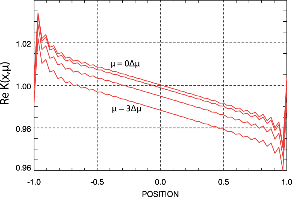
However, we can confirm the presence of the Gibbs phenomenon on $\overline{K}(x,\unicode[STIX]{x1D707},t)$ in the $(x,\unicode[STIX]{x1D707})$-space. Figure 1 gives a typical example in the neighbourhood $\unicode[STIX]{x1D707}\simeq 0$ from an $M=32$ simulation that is discussed below. It would appear that the presence of these spurious oscillations in the middle of the $v$-shift has a potential for introducing error in the simulation.

2.2 Convolution $v$-shift method

To carry out the ‘convolution’ $v$-shift method for updating $\overline{K}_{m}(\unicode[STIX]{x1D707},t)$ one time step $\unicode[STIX]{x0394}t$, the $v$-shift expression (2.7) is integrated directly. We have found that the simple first-order explicit expression

(2.10)$$\begin{eqnarray}\overline{K}_{m}(\unicode[STIX]{x1D707},t+\unicode[STIX]{x0394}t)=\overline{K}_{m}(\unicode[STIX]{x1D707},t)-\text{i}\unicode[STIX]{x03C0}\unicode[STIX]{x1D707}\unicode[STIX]{x0394}t\mathop{\sum }_{n=-M}^{M-1}E_{m-n}\overline{K}_{n}(\unicode[STIX]{x1D707},t)\end{eqnarray}$$

is sufficient for our purposes in this study. Because of the presence of the convolution sum in (2.10), this method is slower than the standard method. Further, the non-uniformity in $\unicode[STIX]{x1D707}$ of the approximation (2.10) limits the allowable values of $\unicode[STIX]{x1D707}_{\text{max}}$ that must satisfy the requirement $\unicode[STIX]{x03C0}\unicode[STIX]{x1D707}_{\text{max}}\unicode[STIX]{x0394}t|E|\ll 1$. To understand the consequence of this limitation, consider the analogue of (2.3) and (2.4) in the Fourier–Fourier transformed space, which is given by

(2.11)$$\begin{eqnarray}\overline{K}_{m}(\unicode[STIX]{x1D707},t)=\unicode[STIX]{x1D6F7}(\unicode[STIX]{x1D707})K_{m}(\unicode[STIX]{x1D707},t),\end{eqnarray}$$

with

(2.12)$$\begin{eqnarray}\unicode[STIX]{x1D6F7}(\unicode[STIX]{x1D707})=\exp \left(-\frac{1}{2}\left(\frac{\unicode[STIX]{x1D707}}{\unicode[STIX]{x1D707}_{f}}\right)^{2}\right).\end{eqnarray}$$

To ensure that recurrence does not arise, we must have $\unicode[STIX]{x1D707}_{f}\ll \unicode[STIX]{x1D707}_{\text{max}}$ (Klimas & Vinas Reference Klimas and Vinas2018). With this bound on the filter width $\unicode[STIX]{x1D707}_{f}$ relative to the limited allowable values for $\unicode[STIX]{x1D707}_{\text{max}}$, we are effectively restricted to low velocity resolution simulations. Even so, this method has the major advantage that with it included the spectral system remains entirely in the Fourier–Fourier transformed space. The evolution of this version of the spectral system cannot be affected by the presence of the Gibbs phenomenon in its $(x,v)$-space output. The argument of Klimas and Viñas (Part 1) applies correctly in this case.

Thus, we have two versions of the spectral simulation system; one containing the suspect $v$-shift step with its excursion into the $(x,\unicode[STIX]{x1D707})$-space and the other providing a reliable basis for comparison. In the following we compare the outputs of these two systems to evaluate the significance of the Gibbs phenomenon in the standard $v$-shift.

3 Standard and convolution spectral simulation comparisons

For all results discussed below, simulations have been carried out on a spatial interval $(-L\leqslant x\leqslant L)$. Time is measured in units of $\unicode[STIX]{x1D714}_{pe}^{-1}$ with $\unicode[STIX]{x1D714}_{pe}$ the electron plasma frequency, length is measured in units of $L$, speed is measured in units of $v_{th}(L/\unicode[STIX]{x1D706}_{D})$ in which $v_{th}$ is the thermal speed and $\unicode[STIX]{x1D706}_{D}=(v_{th}/\unicode[STIX]{x1D714}_{pe})$ is the Debye length. With these choices, the dimensionless distribution function $\overline{f}$ is measured in units of $n_{0}/L\unicode[STIX]{x1D714}_{pe}$ and the dimensionless electric field is measured in units of $4\unicode[STIX]{x03C0}n_{0}L$, in which $n_{0}$ is the one-dimensional density of the stationary background ion distribution; the dimensionless density of the background ion distribution is 1.

We compare the simulation results obtained from the two spectral systems for two simple non-periodic boundary conditions. These are identical to those that appear in Part 1 except that in the transformed space the filter width has been reduced to $\unicode[STIX]{x1D707}_{f}=8$ with $\unicode[STIX]{x1D707}_{\text{max}}=64$. The corresponding velocity filter width is given by $v_{f}=0.04$, compared to the thermal speed $v_{th}=0.16$ used for both examples. Comparisons will be given for $M=32$ and $M=128$.

For the first of these simulations, the ‘steady density gradient’ simulation, a uniform density gradient at fixed temperature is imposed on the initial phase-space distribution and then the density difference at the boundaries that is thereby implied is maintained as time increases. The pressure gradient inherent to the initial state is balanced by a uniform electric field component that remains constant as time increases. For the second simulation, the ‘steady density and temperature gradient’ simulation, a uniform density gradient is again imposed on the initial phase-space distribution but a temperature gradient in the opposite sense is also imposed. In this case, both the temperature and density differences at the boundaries contained in the initial state are maintained as time increases. The gradients are adjusted so that there is no net pressure gradient in the plasma; a uniform electric field is not imposed. The considerable activity that occurs in both examples as the plasmas evolve into new equilibrium states is described in detail in Part 1.

3.1 Steady density gradient

For the first non-periodic solution example, we consider an electron plasma whose initial space-averaged phase-space distribution is given by the thermal distribution

(3.1)$$\begin{eqnarray}f_{0}(v,t=0)=\frac{1}{v_{th}\sqrt{2\unicode[STIX]{x03C0}}}\exp \left(-\frac{1}{2}\left(\frac{v}{v_{th}}\right)^{2}\right),\end{eqnarray}$$

with, following Cheng & Knorr (Reference Cheng and Knorr1976), $v_{th}=0.5/\unicode[STIX]{x03C0}$. We assume that the initial phase-space distribution is given by

(3.2)$$\begin{eqnarray}f(x,v,t=0)=f_{0}(v,t=0)\left(1+\frac{\unicode[STIX]{x1D6FC}}{2}x\right)\end{eqnarray}$$

and therefore

(3.3)$$\begin{eqnarray}\unicode[STIX]{x1D6FF}f(v,t=0)\equiv f(x=1,v,t=0)-f(x=-1,v,t=0)=\unicode[STIX]{x1D6FC}f_{0}(v,t=0).\end{eqnarray}$$

For this example, the distribution difference at the spatial boundaries is held constant, $\unicode[STIX]{x1D6FF}f(v,t)=\unicode[STIX]{x1D6FF}f(v,t=0)$, and the strength of that difference is fixed by the parameter $\unicode[STIX]{x1D6FC}$. For the ‘steady density gradient solution’ discussed in this section, $\unicode[STIX]{x1D6FC}=0.12$ (note: in Part 1 it is stated that $\unicode[STIX]{x1D6FC}=0.06$ but this is the value that was actually used).

Figure 2.

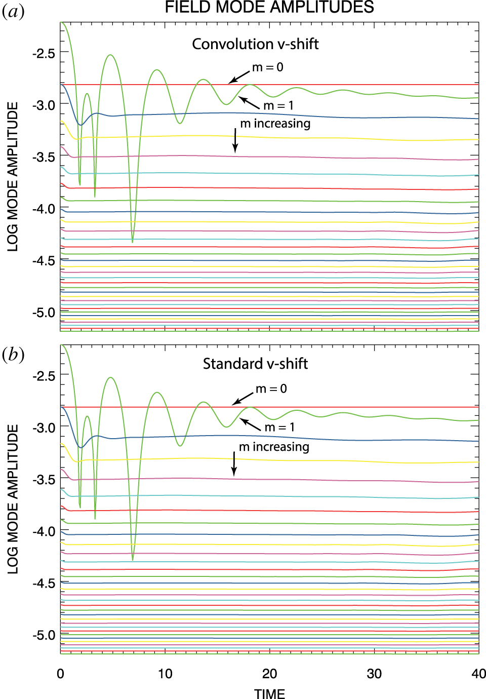
Field-mode magnitude evolution for $M=32$ (a) convolution $v$-shift simulation and (b) standard $v$-shift simulation of the steady density gradient solution.

3.1.1 Electric field-mode amplitudes

Two simulations of the steady density gradient solution have been carried out with each of the standard and convolution spectral systems; for the first of these $M=32$ and for the second $M=128$. The evolution with time of the electric field-mode magnitudes from the $M=32$ simulations are shown in figure 2. Results from the convolution spectral system are shown in (a) and those from the standard system are shown in (b). The red curve labelled $m=0$ in each of the panels of the figure confirms the expected lack of evolution with time of $E_{0}(t)$. Agreement between results in the two panels is excellent; differences are non-discernible at the graphical level shown. It is important to note that the highest $m$-value, shortest wavelength modes shown are several hundred times smaller than the dominant mode. The $M=128$ results are not shown since they are essentially identical to these for the first 32 modes while the remainder of the $M=128$ mode are of even smaller amplitudes. We can conclude that the electric field $E(x,t)$ is effectively identical in all four of the simulations under discussion; $M=32$, $M=128$, convolution $v$-shift and standard $v$-shift. In addition, for the overall charge-neutral solutions under consideration here, the electric field remains continuous at the spatial boundaries (Part 1). The field does not exhibit the Gibbs phenomenon.

3.1.2 Phase-space distributions

For a high velocity resolution version of this steady density gradient solution, Klimas and Viñas (Part 1) have shown that, in addition to the electric field, the density and temperature moments of the phase-space distributions obtained from the standard spectral system and a flux-balance system that operates fully in the $(x,v)$-space are in precise agreement. Here, we add to this result by comparing the phase-space distributions obtained from the standard and convolution spectral systems directly.

Figure 3.

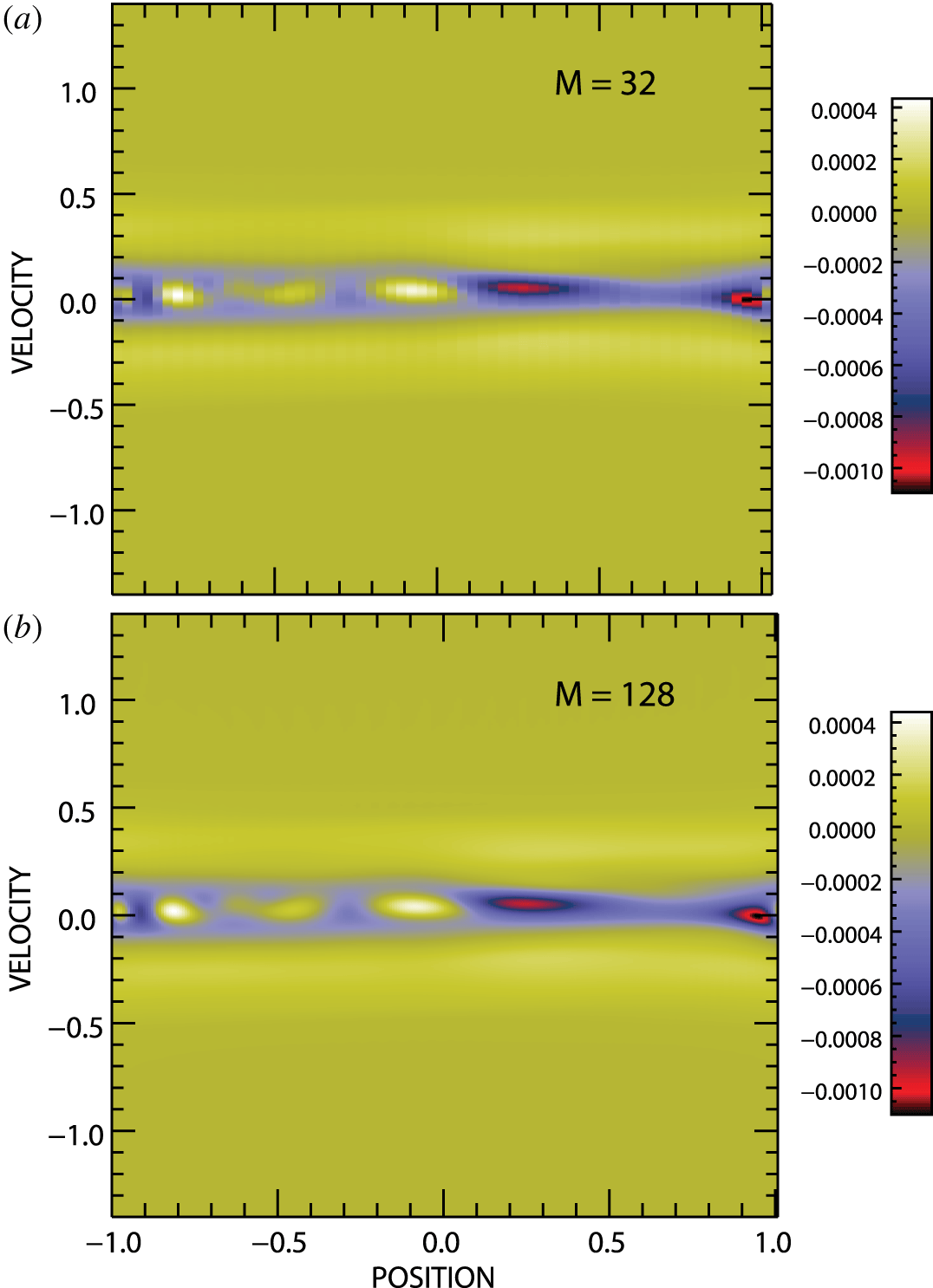
Phase-space distribution differences from standard and convolution spectral simulations of the steady density gradient solution at $t=30$ for (a) $M=32$ and (b) $M=128$.

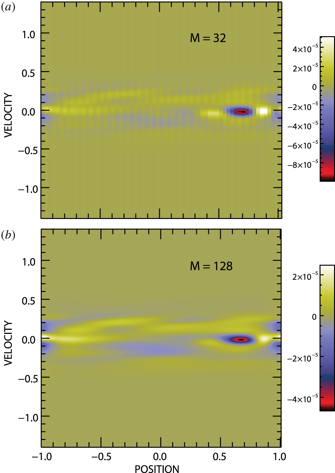
Figure 3 shows, at time $t=30$, the differences between the phase-space distributions obtained from the standard and convolution simulations of the steady density gradient solution for $M=32$ and $M=128$. It can be seen that the differences peak in the vicinity of $v=0$ where the actual distributions peak at approximately 2.5 (e.g. see figures 5, 6 and 7 of Part 1). By this measure, or when compared to the strength of the gradient imposed on this non-periodic simulation, $\unicode[STIX]{x1D6FF}f(v,t)=0.12f_{0}(v,t=0)$, the differences between the distributions for $M=32$ and $M=128$ are similar and small.

3.2 Steady density and temperature gradients

For our second non-periodic simulation example we consider an electron plasma whose initial state is the spatially dependent thermal distribution

(3.4)$$\begin{eqnarray}f(x,v,t=0)=\left(1+\frac{\unicode[STIX]{x1D6FC}}{2}x\right)\frac{1}{v_{th}(x)\sqrt{2\unicode[STIX]{x03C0}}}\exp \left(-\frac{1}{2}\left(\frac{v}{v_{th}(x)}\right)^{2}\right),\end{eqnarray}$$

with

(3.5)$$\begin{eqnarray}v_{th}(x)=v_{th0}\sqrt{1+\frac{\unicode[STIX]{x1D6FD}}{2}x},\end{eqnarray}$$

in which $\unicode[STIX]{x1D6FD}$ is a free parameter that controls the strength of the temperature gradient and, following Cheng & Knorr (Reference Cheng and Knorr1976), $v_{th0}=0.5/\unicode[STIX]{x03C0}$. In this case

(3.6)$$\begin{eqnarray}\displaystyle \unicode[STIX]{x1D6FF}f(v,t=0) & = & \displaystyle f(1,v,t=0)-f(-1,v,t=0)\nonumber\\ \displaystyle & = & \displaystyle \frac{(1+\unicode[STIX]{x1D6FC}/2)}{v_{th0}\sqrt{2\unicode[STIX]{x03C0}(1+\unicode[STIX]{x1D6FD}/2)}}\exp \left(-\frac{1}{2(1+\unicode[STIX]{x1D6FD}/2)}\left(\frac{v}{v_{th0}}\right)^{2}\right)\nonumber\\ \displaystyle & & \displaystyle -\,\frac{(1-\unicode[STIX]{x1D6FC}/2)}{v_{th0}\sqrt{2\unicode[STIX]{x03C0}(1-\unicode[STIX]{x1D6FD}/2)}}\exp \left(-\frac{1}{2(1-\unicode[STIX]{x1D6FD}/2)}\left(\frac{v}{v_{th0}}\right)^{2}\right)\end{eqnarray}$$

and, again, we set $\unicode[STIX]{x1D6FF}f(v,t)=\unicode[STIX]{x1D6FF}f(v,t=0)$. For this distribution, the pressure difference across the spatial domain is given by

(3.7)$$\begin{eqnarray}\unicode[STIX]{x1D6FF}P=\int _{-\infty }^{\infty }\,\text{d}vv^{2}\unicode[STIX]{x1D6FF}f(v,t=0)=v_{th0}^{2}(\unicode[STIX]{x1D6FD}+\unicode[STIX]{x1D6FC}).\end{eqnarray}$$

We choose $\unicode[STIX]{x1D6FC}=-\unicode[STIX]{x1D6FD}=-0.06$ (again: the values stated in Part 1 are $\unicode[STIX]{x1D6FC}=-\unicode[STIX]{x1D6FD}=-0.03$ but these are the values that were used). to obtain $\unicode[STIX]{x1D6FF}P=0$ and therefore, with $u_{0}(t=0)=0$ we have $E_{0}(t)=E_{0}(t=0)=0$ (Part 1). This ‘steady density and temperature gradient solution’ remains in overall pressure equilibrium for $t\geqslant 0$ using density and temperature gradients in opposing directions.

3.2.1 Electric field-mode amplitudes

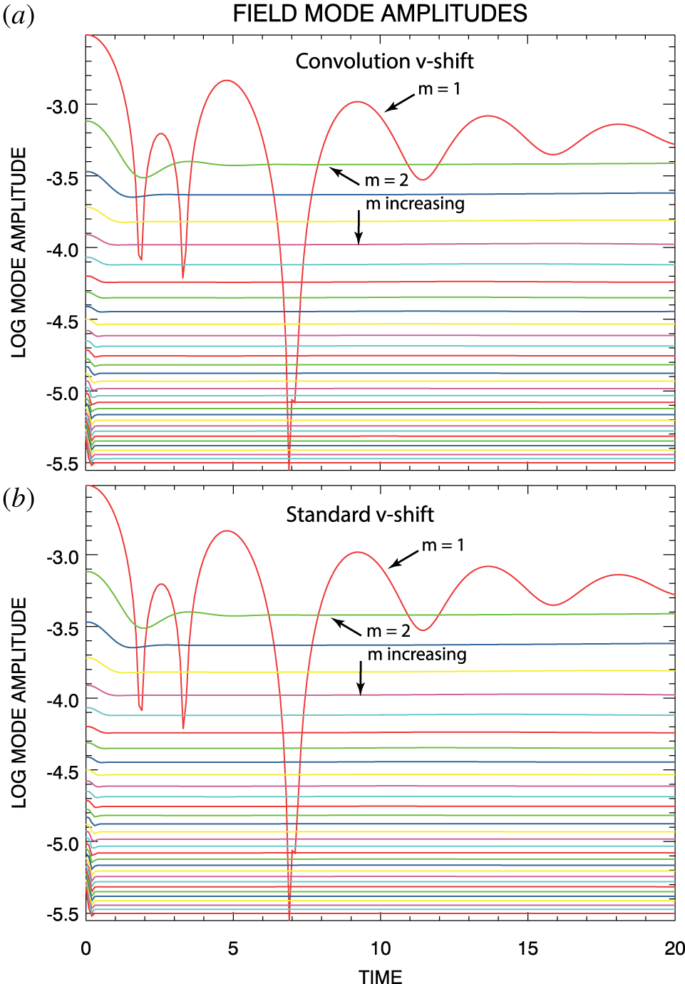
For this second non-periodic example, two simulations of the steady density and temperature gradient solution have been carried out with each of the standard and convolution spectral systems; for the first of these $M=32$ and for the second $M=128$. The evolution with time of the electric field-mode magnitudes from the $M=32$ simulations are shown in figure 4. Results from the convolution spectral system are shown in (a) and those from the standard system are shown in (b). In this case, $E_{0}(t)=0$ and, thus, it does not show up. Agreement between results in the two panels is excellent; differences are non-discernible at the graphical level shown. In this case, it is also true that the highest $m$-value, shortest wavelength modes shown are several hundred times smaller than the dominant mode. Again, the $M=128$ results are not shown since they are essentially identical to these for the first 32 modes while the remainder of the $M=128$ mode are of even smaller amplitudes. Once again, we conclude that the electric field $E(x,t)$ is effectively identical in all four of the simulations under discussion; $M=32$, $M=128$, convolution $v$-shift, and standard $v$-shift. As explained above, the electric field remains continuous at the spatial boundaries (Part 1). The field does not exhibit the Gibbs phenomenon.

Figure 4.

Field-mode magnitude evolution for $M=32$ (a) convolution $v$-shift simulation and (b) standard $v$-shift simulation of the steady density and temperature gradient solution.

3.2.2 Phase-space distributions

For a high velocity resolution version of this steady density gradient solution, Klimas and Viñas (Part 1) have shown that, in addition to the electric field, the density and temperature moments of the phase-space distributions obtained from the standard spectral system and a flux-balance system that operates fully in the $(x,v)$-space are in precise agreement. Here, we add to this result by comparing the phase-space distributions obtained from the standard and convolution spectral systems directly.

Figure 5.

Phase-space distribution differences from standard and convolution spectral simulations of the steady density and temperature gradient solution at $t=20$ for (a) $M=32$ and (b) $M=128$.

Figure 5 shows, at time $t=20$, the differences between the phase-space distributions obtained from the standard and convolution simulations of the steady density and temperature gradient solution for $M=32$ and $M=128$. As in the case of the steady density gradient simulations, it can be seen that the differences peak in the vicinity of $v=0$ where the actual distributions peak at approximately 2.5 (e.g. see figures 5, 6 and 7 of Part 1). By this measure, or when compared to the strength of the gradient imposed on this non-periodic simulation the differences between the distributions for both $M=32$ and $M=128$ are small. In contrast to the steady density gradient simulations, the differences between the phase-space distributions for $M=128$ are approximately half those of the $M=32$ simulations.

4 The $v$-shift spectral simulations

It is important to understand in more generality the influence that the Gibbs phenomenon may have in the $v$-shift step of the standard spectral system. We must wonder what errors might develop in longer, more physical non-periodic spectral system simulations and whether those errors would be recognizable for what they are. In this section, we show that the effects on the phase-space distribution of the Gibbs oscillations within the $v$-shift step of the standard spectral system can be isolated, recognized and likely mitigated.

We have reduced the standard and convolution spectral systems to solely their $v$-shift step, which we have applied repeatedly with an unvarying electric field. Then, after $n$ such applications we have in $(x,v)$-space

(4.1)$$\begin{eqnarray}\overline{f}(x,v,t)=\overline{f}(x,v+E(x)n\unicode[STIX]{x0394}t,0)\quad t=n\unicode[STIX]{x0394}t.\end{eqnarray}$$

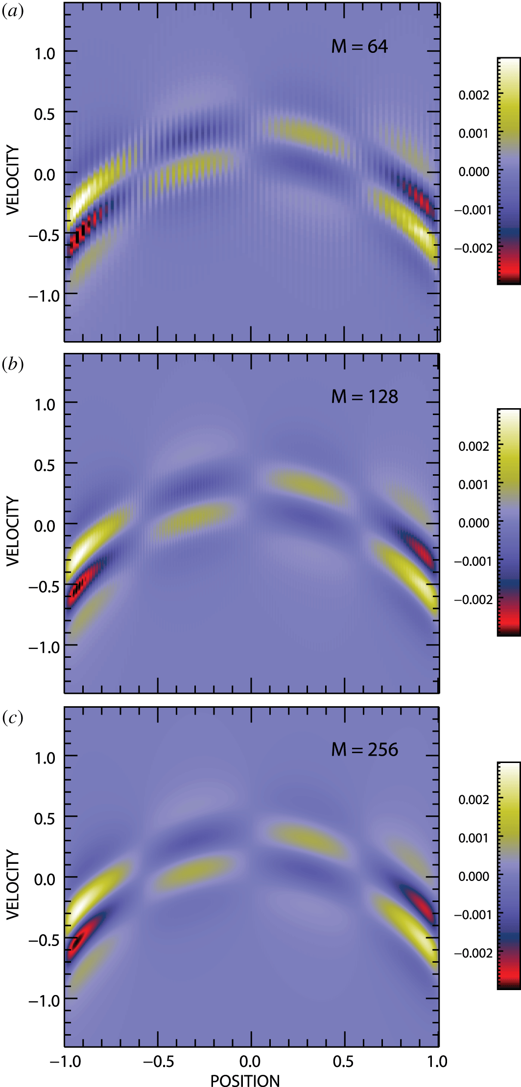
Figure 6 shows the differences that develop between the phase-space distributions of the two spectral systems at $n=800$ and $\unicode[STIX]{x0394}t=0.1$ for $M=64$, $M=128$ and $M=256$ using $\overline{f}(x,v,0)$ and $E(x)$ captured from early in the steady density and temperature gradient simulations.

We find two important features in figure 6. First, there is the same unvarying background distribution of differences in each of the panels. These differences are independent of the number of spatial Fourier modes $M$ used in each of the simulations. Second, there are spatial oscillations superposed on top of the background distribution that are quite evident at $M=64$, just barely visible at $M=128$, and not discernible at $M=256$. The appearance of these oscillations clearly does depend on the number of spatial Fourier modes $M$ used in each of the simulations.

Figure 6.

Phase-space distribution differences from standard and convolution spectral simulations of the steady $v$-shift solution at $t=80$ for (a) $M=64$, (b) $M=128$ and (c) $M=256$.

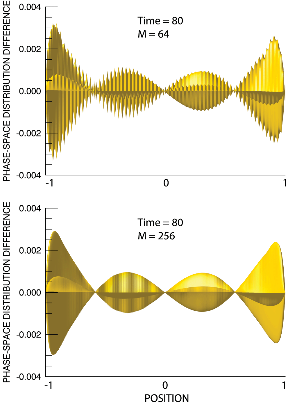
Figure 7 shows a different view of the standard and convolution spectral phase-space differences at $t=80$ for $M=64$ in (a) and at $M=256$ in (b). These are surface plots seen edge on of the differences shown in the top and bottom panels of figure 6. The view is along the $v$-axis from nearby in the negative $v$ direction. The superposition of spatial oscillations on top of the background distribution is evident for $M=64$. We can confirm that the oscillations, at higher frequency and lower amplitude, are still there in the $M=256$ case. Clearly, the oscillations are $M$ dependent. In addition, this figure further supports our conclusion that the background distribution of differences is $M$ independent.

Figure 7.

Surface plots of the phase-space differences obtained from the $v$-shift simulations of the standard and convolution spectral systems for (a) $M=64$ and (b) $M=256$. The surfaces are viewed edge on along the $v$-axis from the negative $v$ direction.

We have shown in § 3 that the shortest wavelength, highest $m$-value field modes, even in the case $M=32$, are very weak in comparison to the dominant long wavelength modes. All of the higher $M$ simulations reproduce the field-mode distribution of the $M=32$ simulation while adding more shorter wavelength, much weaker modes to the field. We can conclude that the electric field producing the $v$-shift (4.1) in these $v$-shift-only simulations is effectively identical in all of the simulations. Neglecting, for the moment, the possible effects of the Gibbs phenomenon in the $v$-shift of the standard spectral code, we should expect that whatever differences develop between the standard and convolution spectral simulation results would be $M$ independent.

Conversely, we do know that the spatial distribution of the Gibbs phenomenon depends strongly on the number of Fourier modes $M$. Thus, if the Gibbs phenomenon in the standard $v$-shift has any signature in a simulation output, we should expect that signature would be $M$ dependent.

Thus, we conclude: (i) the unvarying $M$ independent background distribution of differences in figures 6 and 7 is the inherent difference that develops between the two spectral simulation techniques, irrespective of the presence of the Gibbs phenomenon in the standard $v$-shift; (ii) the position- and $M$-dependent oscillations that appear superposed on that background distribution represent the effects of the Gibbs phenomenon in the standard $v$-shift; (iii) these oscillations are clearly identifiable if/when they arise.

For example, it can be seen that the spatial oscillations are, in fact, discernible in the $M=32$ differences shown in figures 3 and 5 for the non-periodic simulations discussed there. We have shown that these effects may be controllable with additional spatial Fourier modes, as in figures 3 and 5–7. Results from future studies of non-periodic spectral system simulations will be reported.