2.1. Inverse formulation of the non-similar boundary-layer problem

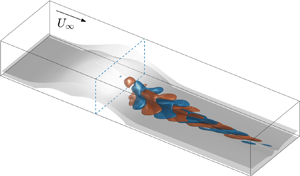
Figure 1 illustrates the geometry of the model problem. The dimensional streamwise, wall-normal and spanwise coordinates are denoted by $x^{*}$, $y^{*}$ and $z^{*}$, and their respective velocity components by $u^{*}, v^{*}$ and $w^{*}$. Dimensionless magnitudes, to be defined later, follow the same nomenclature but the superscript $*$ is dropped. The boundary-layer edge velocity $U_e ^{*}$ and the kinematic viscosity $\nu ^{*}$ are used to define the boundary-layer coordinates $\xi = x^{*} / L^{*}$ and $\eta = y^{*} \sqrt {U_e ^{*} / \nu ^{*} x^{*}}$, and the transformed streamfunction

(2.1)\begin{equation} f(\xi,\eta) = \varPsi^{*} / \sqrt{U_e ^{*} \nu^{*} x^{*}}. \end{equation}

The dimensional streamfunction is denoted by $\varPsi ^{*}$ and $L^{*}$ is an arbitrary scale length. After substitution of these variables in the streamwise momentum equation, the following equation for $f(\xi ,\eta )$ is obtained:

(2.2)\begin{equation} f_{\eta\eta\eta} + \frac{m+1}{2} f f_{\eta\eta} +m(1-f_{\eta} ^{2}) = \xi (\varTheta f_{\eta} f_{\xi \eta} + f_{\eta \eta} f_{\xi}). \end{equation}

Subscripts denote partial differentiation, and $m = (\xi / U_e ^{*})( \mbox {d} U_e ^{*} / \mbox {d} \xi )$ quantifies the free-stream pressure gradient, which only depends on $\xi$ (Schlichting Reference Schlichting1979). In order to recover separated states, the so-called FLARE approximation (Reyhner & Flügge-Lotz Reference Reyhner and Flügge-Lotz1968; Carter Reference Carter1975) is invoked, that neglects the streamwise convective term when reversed flow exists. The FLARE approximation appears in this equation as the function $\varTheta (\xi ,\eta )$, which takes value unity when $f_\eta \ge 0$ and vanishes if $f_\eta < 0$. Equation (2.2) is complemented with the boundary conditions

(2.3a–c)\begin{equation} f(\xi,0) = 0, \quad f_{\eta}(\xi,0) = 0, \quad \textrm{and} \quad f_{\eta}(\xi,\eta \rightarrow \infty) \rightarrow 1. \end{equation}

Figure 1.

Problem geometry and computational domain.

The direct formulation of the non-similar boundary-layer equations prescribes a distribution of the boundary-layer edge velocity $U^{*} _e(\xi )$ or the external-flow pressure gradient $m(\xi )$. However, this approach fails when a point of vanishing wall shear is reached, a phenomenon that is known as Goldstein's singularity (Howarth Reference Howarth1934). An inverse formulation is used here to circumvent the singularity; the displacement thickness distribution $\bar {\delta }(\xi )$ is imposed as the missing boundary condition

(2.4)\begin{equation} f(\xi,\eta \rightarrow \infty) \rightarrow 1 - \bar{\delta}(\xi). \end{equation}

The solution algorithm marches downstream and iterates on each $\xi$ profile until a converged solution profile $f(\xi ,\eta )$ and $m(\xi )$ are obtained. The inverse-problem formulation recovers the boundary-layer edge velocity $U^{*} _e(\xi )$ corresponding to the imposed displacement thickness distribution $\bar {\delta }(\xi )$, accounting for the viscous–inviscid interaction effects that cause Goldstein's singularity. Details on the numerical solution can be found in Rodríguez (Reference Rodríguez2010).

2.2. Construction of the baseline laminar separation bubbles

An analytical displacement thickness distribution analogous to that prescribed by Carter (Reference Carter1975) is imposed in (2.4). The solution of (2.2) is initiated with the velocity profile and $\bar {\delta }$ value corresponding to the Blasius solution ($\bar {\delta }_{B}=1.72078$). The displacement thickness is increased over a finite extent along the streamwise direction, following an analytical expression that can be found in Rodríguez & Theofilis (Reference Rodríguez and Theofilis2010b).

In what follows, lengths and velocities are scaled respectively with the displacement thickness $\delta ^{*} _{in}$ and the free-stream velocity $U^{*} _{in}$ at a streamwise location upstream of the increase of $\bar {\delta }$. This location is chosen so that the Reynolds number based on the local displacement thickness is $Re = 450$, which is comparable with that in reported direct numerical simulations (Rist & Maucher Reference Rist and Maucher1994; Alam & Sandham Reference Alam and Sandham2000; Spalart & Strelets Reference Spalart and Strelets2000). Setting the arbitrary length $L^{*} = \delta ^{*} _{in}$ leads to $\xi = x$. The increase of the displacement thickness over the Blasius value starts at a coordinate $x _1$ and returns to the Blasius value at $x_2$. In boundary-layer coordinates, the function $\bar {\delta }(x)$ is symmetric about the coordinate $x_\delta = (x_1 + x_2)/2$, where it reaches its peak value, $\bar {\delta }_{max}$. Thus, $\bar {\delta }(x)$ is completely defined by the parameters $x_1, x_2$ and $\bar {\delta }_{max}$. While $\bar {\delta }$ is symmetric, the resulting recirculation bubble is highly asymmetric and the locations of the peak negative wall shear and streamwise velocity are displaced towards the reattachment point. Prescribing an increase in the displacement thickness over the Blasius value is equivalent to imposing an adverse pressure gradient or a deceleration of the free stream, and these terms will be employed indistinctly in the rest of the paper.

Using the same approach, Rodríguez et al. (Reference Rodríguez, Gennaro and Juniper2013b) computed a series of baseline separation bubbles considering three different extents of the free-stream deceleration. For each extent, the value $\bar {\delta }_{max}$ was varied from 3 to 10 to generate a large number of different LSBs. In the present work, we consider only the family of model bubbles corresponding to the longest streamwise extent, defined by $x_1 = 210, x_2 = 320$ and varying $\bar {\delta }_{max}$.

The baseline two-dimensional LSBs in this study are constructed to be quantitatively comparable with other separation bubbles in the literature. Three magnitudes are computed for comparison: (i) the Reynolds number based on the momentum thickness and edge velocity at separation $Re_{\theta ,s} = \theta ^{*}_s U^{*}_{e,s} / \nu ^{*}$, which lies in the range 208–212; the Reynolds number based on the length of the recirculation region and free-stream velocity $Re_L = (x^{*}_r - x^{*}_s) U^{*}_{in} / \nu ^{*}$ (where $x^{*}_r$ and $x^{*}_s$ are the dimensional reattachment and separation locations), which is between 37 600 and 40 500; and (iii) the peak reversed flow scaled with the free-stream velocity, $u_{rev} = - {{\rm min}}(u^{*})/U^{*}_{in}$. Figure 2(a) shows the variation of the peak reversed flow in the baseline LSBs, $u_{0,rev}$ with $\bar {\delta }_{max}$ (subscript $0$ is used to denote the flow fields corresponding to the baseline LSBs). The maximum reversed flow that can be obtained with the boundary-layer formulation is $u_{0,rev} \approx 12\,\%$. This value corresponds to the peak reversed flow attainable in Falkner–Skan profiles, which are asymptotic solutions of the present formulation (Schlichting Reference Schlichting1979).

Figure 2.

(a) Dependence of the peak reversed flow in the baseline LSB, $u_{0,rev}$, with the maximum displacement thickness, $\bar {\delta }_{max}$. (b) Neutral curve for the primary instability eigenmode (solid line) and spanwise wavenumber of maximum growth rate (dashed line).

3.1. Modal linear instability analyses

Three-dimensional flows of viscous incompressible fluids are described by the continuity and Navier–Stokes equations

(3.1a,b)\begin{equation} \boldsymbol{\nabla} \boldsymbol{\cdot} \boldsymbol{v} = 0, \quad \frac{\partial \boldsymbol{v}}{\partial t} + \boldsymbol{v} \boldsymbol{\cdot} \boldsymbol{\nabla} \boldsymbol{v} = - \boldsymbol{\nabla} p + \frac{1}{Re}\nabla^{2} \boldsymbol{v}, \end{equation}

where $\boldsymbol {v} = (u,v,w)$ is the velocity field, $p$ is the reduced pressure and $Re$ is the Reynolds number, as defined in § 2.

Let $\boldsymbol {q} = (\boldsymbol {v},p)$ be the total flow field. Linear stability theory studies the evolution of infinitesimally small disturbances $\boldsymbol {q}'$ superimposed to a base flow $\bar {\boldsymbol {q}}$. The total flow field is decomposed as

(3.2)\begin{equation} \boldsymbol{q}(x,y,z,t) = \bar{\boldsymbol{q}}(x,y,z) + \epsilon \boldsymbol{q}'(x,y,z,t), \end{equation}

where $\epsilon \ll 1$. Substitution of (3.2) on the Navier–Stokes equations and linearization about the steady base flow results on the linearized Navier–Stokes equations, that can be recast in matrix form as

(3.3)\begin{equation} {\boldsymbol{\mathsf{B}}} \frac{\partial \boldsymbol{q}'}{\partial t} = {\boldsymbol{\mathsf{A}}}_{3D}\,\boldsymbol{q}'. \end{equation}

The linear operators ${\boldsymbol{\mathsf{A}}}_{3D}$ and ${\boldsymbol{\mathsf{B}}}$ depend on the base flow components and their spatial derivatives and on the Reynolds number, but not on time. This allows for the introduction of the modal form

(3.4)\begin{equation} \boldsymbol{q}'(x,y,z,t) = \hat{\boldsymbol{q}}(x,y,z) \exp(-\mbox{i} \omega t) + \textrm{c.c}., \end{equation}

with c.c. denoting the complex conjugate, which results in the generalized eigenvalue problem (EVP)

(3.5)\begin{equation} -\mbox{i} \omega {\boldsymbol{\mathsf{B}}} \, \hat{\boldsymbol{q}}(x,y,z) = {\boldsymbol{\mathsf{A}}}_{3D}(\bar{\boldsymbol{q}}(x,y,z),Re) \, \hat{\boldsymbol{q}}(x,y,z), \end{equation}

where $\omega$ are the eigenvalues and $\hat {\boldsymbol {q}}$ the eigenfunctions.

The real part of the eigenvalues $\omega _r$ corresponds to a circular frequency of oscillation while the imaginary part $\omega _i$ is the growth rate. If all the eigenmodes have $\omega _i <0$, then any disturbance introduced in the flow decays asymptotically for long times and the base flow is said to be linearly stable. Conversely, if $\omega _i > 0$ for at least one eigenmode, the base flow is unstable and the flow field evolves towards a different state.

In the most general case, when the base flow depends explicitly on the three spatial directions, so do the linear operators and the eigenfunctions; this EVP is known as three-dimensional eigenmode analysis or tri-global analysis (Theofilis Reference Theofilis2011). Many problems of interest exist in which the base flow depends only on one or two spatial directions, enabling the introduction of Fourier modes on these directions and reducing substantially the complexity of the problem. Two such simplifications are relevant to the present work.

3.1.1. Three-dimensional global eigenmodes of a two-dimensional non-parallel flow

In the analysis of the primary instability to be discussed in § 4, the base flow corresponds to the baseline two-dimensional LSBs $\boldsymbol {q}_0$ (described in § 2), which are homogeneous on the spanwise direction $z$. Spanwise-periodic eigenmodes are then introduced, of the form

(3.6)\begin{equation} \boldsymbol{q}'(x,y,z,t) \sim \hat{\boldsymbol{q}}(x,y) \exp[\mbox{i}(\beta z - \omega t)] + \textrm{c.c.}, \end{equation}

where $\beta$ is a wavenumber associated with the spanwise periodicity length $\lambda _z = 2 {\rm \pi}/ \beta$. This modal form simplifies the EVP to a two-dimensional one, identical to the one solved by e.g. Theofilis et al. (Reference Theofilis, Hein and Dallmann2000) or Barkley et al. (Reference Barkley, Gomes and Henderson2002)

(3.7)\begin{equation} -\mbox{i} \omega {\boldsymbol{\mathsf{B}}} \, \hat{\boldsymbol{q}}(x,y) = {\boldsymbol{\mathsf{A}}}_{2Dz}(\bar{\boldsymbol{q}}(x,y),\beta,Re)\, \hat{\boldsymbol{q}}(x,y). \end{equation}

The linear operator ${\boldsymbol{\mathsf{A}}}_{2Dz}$ is obtained from ${\boldsymbol{\mathsf{A}}}_{3D}$ by imposing a base flow of the form $\bar {\boldsymbol {q}}(x,y)$ with $\bar {w}=0$, and modal disturbances of the form (3.6). The resulting EVP must be complemented with adequate homogeneous boundary conditions, that will be discussed in § 4.

3.1.2. Global oscillator analysis based on cross-stream planes

A different simplification is used in § 5, in which the base flow corresponds to steady three-dimensional separation bubbles. A weakly non-parallel approximation is introduced, based on the assumption that the spatial scale $L$ on which streamwise variations of the base flow are significant is large compared to those on the cross-stream section and to the instability wavelengths $\lambda _x = 2{\rm \pi} /\alpha _r$. Evidence has been amassed that this approximation is valid for instability waves developing over laminar separation bubbles (Dovgal et al. Reference Dovgal, Kozlov and Michalke1994; Rist & Maucher Reference Rist and Maucher2002; Diwan & Ramesh Reference Diwan and Ramesh2012). Local instability analyses based on the weakly non-parallel approximation can be used to study the existence of self-excited instabilities consisting of synchronized oscillations across the flow field. When such an oscillator-type instability is present, weakly non-parallel analysis delivers results analogous to the more expensive global eigenmode computation (Pier Reference Pier2002; Giannetti & Luchini Reference Giannetti and Luchini2007; Pier Reference Pier2008; Juniper, Tammisola & Lundell Reference Juniper, Tammisola and Lundell2011; Siconolfi et al. Reference Siconolfi, Citro, Giannetti, Camarri and Luchini2017). The weakly non-parallel analysis proposed by Chomaz et al. (Reference Chomaz, Huerre and Redekopp1988) and Huerre & Monkewitz (Reference Huerre and Monkewitz1990), based on the Wentzel–Kramers–Brillouin–Jeffrey (WKBJ) approximation, is extended here to three-dimensional base flows which have a strong dependence on the two cross-stream directions. Only the main elements of the approach are described; a more detailed explanation can be found in Huerre & Monkewitz (Reference Huerre and Monkewitz1990) and Siconolfi et al. (Reference Siconolfi, Citro, Giannetti, Camarri and Luchini2017).

The slow coordinate $X = \gamma x$ is defined, with $\gamma = \lambda _x / L$ assumed to be a small quantity. At each $X$-plane, the instability waves are locally described by the modal form

(3.8)\begin{equation} \boldsymbol{q}'(x,y,z,t) \sim \hat{\boldsymbol{q}}(X,y,z) \exp[\mbox{i}(\alpha(X) x - \omega t)] + \textrm{c.c.} \end{equation}

leading to a generalized EVP of the form

(3.9)\begin{equation} -\mbox{i} \omega {\boldsymbol{\mathsf{B}}} \, \hat{\boldsymbol{q}}(y,z) = {\boldsymbol{\mathsf{A}}}_{2Dx}(\alpha,\bar{\boldsymbol{q}}(X,y,z)) \, \hat{\boldsymbol{q}}(y,z). \end{equation}

The linear operator ${\boldsymbol{\mathsf{A}}}_{2Dx}$ is obtained by substituting the disturbance form (3.8) in ${\boldsymbol{\mathsf{A}}}_{3D}$. Following Siconolfi et al. (Reference Siconolfi, Citro, Giannetti, Camarri and Luchini2017), terms proportional to first-order streamwise derivatives of the base flow quantities are retained. These additional $O(\gamma )$ terms have a small effect on the local stability properties of the flow, but their inclusion simplifies the numerical evaluation of the global frequency correction, described below.

In the analysis of local instability waves, both the streamwise wavenumber and the frequency can take complex values, i.e. $\omega = \omega _r + \mbox {i} \omega _i$ and $\alpha = \alpha _r + \mbox {i} \alpha _i$. The solution of this EVP delivers a complete eigenspectrum, from which only a small number of discrete eigenmodes correspond to potentially unstable waves. Successive solutions of (3.9) can be used to map the individual eigenmodes from the complex plane $\alpha$ to the complex plane $\omega$ at each $X$, establishing the dispersion relation $D(\alpha ,\omega ,X) = 0$. This dispersion relation governs the evolution of packets of disturbance waves (i.e. wavepackets) locally at the cross-stream plane $X$.

The analysis proceeds by determining, at each $X$-plane, the complex frequency associated with disturbance waves with zero group velocity $c_g = \partial \omega / \partial \alpha$. This frequency is known as the local absolute frequency $\omega _0 (X)$, and the associated wavenumber is denoted by $\alpha _0 (X)$. A temporally amplified absolute frequency ($\omega _{0,i} > 0$) implies instability waves that grow in amplitude while propagating upstream. The base flow is then said to be absolutely unstable locally at the $X$-plane, as opposed to convectively unstable conditions for which only downstream propagating waves grow in amplitude.

If the streamwise portion of the base flow being absolute unstable is sufficiently large, a self-exciting mechanism can exist leading to synchronized oscillations, characterized by the complex global oscillation frequency

(3.10)\begin{equation} \omega_g = \omega_s + \gamma \omega_\gamma. \end{equation}

The leading-order contribution $\omega _s$ is given by the saddle point of $\omega _0 (X)$ on the complex $X$-plane, $\mbox {d} \omega _0 / \mbox {d} X = 0$. The complex $X$ coordinate that satisfies this condition is referred to as the wavemaker $X_s$ and $\omega _s = \omega _0(X_s)$. The correction term $\omega _\gamma$ will be discussed shortly below.

The spatial structure of the oscillator is calculated by investigating how the flow responds to the saddle-point frequency, i.e. by evaluating

(3.11)\begin{equation} \boldsymbol{q}'(x,y,z,t) \sim \varPsi_0(X) \hat{\boldsymbol{q}}^{\pm}(y,z;X,\omega_s) \exp \left( \frac{\mbox{i}}{\gamma} \int_X \alpha^{\pm}(X',\omega_s) \,\mbox{d} X' - \mbox{i} \omega_g t\right) + \textrm{c.c.} \end{equation}

The results of the local EVP are used at each $X$-plane: $\alpha ^{-}$ and $\alpha ^{+}$ are respectively the upstream- and downstream-propagating local wavenumbers, which are considered at each side of the wavemaker $X_s$ and satisfy (3.9) for $\omega = \omega _s$. Similarly, $\hat {\boldsymbol {q}}^{\pm }$ are the corresponding local eigenfunctions associated with $\alpha ^{\pm }$. The global oscillator structure is computed by integrating the $\alpha ^{-}$ branch upstream of $X_s$ and the $\alpha ^{+}$ downstream of $X_s$. The WKBJ approximation breaks down in a small region around the saddle point, for which a different scaling of the streamwise variables and disturbance form are required (Huerre & Monkewitz Reference Huerre and Monkewitz1990). The asymptotic matching of the outer $\alpha ^{-}$ and $\alpha ^{+}$ solutions and the inner WKBJ solution determines the values admitted by the correction term $\omega _\gamma$:

(3.12)\begin{equation} \omega_\gamma = -\frac{\mbox{i}}{2} \omega_{\alpha\alpha} \alpha_{0,X} + ( \omega_{0,XX} \omega_{\alpha\alpha})^{1/2} \left( n + 1/2\right), \end{equation}

where $\omega _{\alpha \alpha } = \partial ^{2} \omega / \partial \alpha ^{2}$, $\alpha _{0,X} = \partial \alpha _0 / \partial X$ and $\omega _{0,XX} = \partial ^{2} \omega _0 / \partial X^{2}$, all of them evaluated at the saddle point $X_s$. The non-negative integer $n$ accounts for different matching solutions. The value $n=0$ is chosen for all the computations in this paper, as it corresponds to the solution with a larger growth rate. The scalar function $\varPsi _0(X)$ in (3.11) is determined from the matching of the inner and outer solutions. However, Juniper et al. (Reference Juniper, Tammisola and Lundell2011) showed that the error incurred in assuming a uniform value for $\varPsi _0$ is smaller than the influence of the inaccuracies in $\alpha ^{\pm }$. Consequently, $\varPsi _0$ is taken as uniform here too.

3.2. Direct numerical simulations

Direct numerical simulations (DNS) are performed to validate the results of the linear analyses and to study the nonlinear regimes. The main characteristics of the code employed are summarized here; the complete description of the methodology and validations can be found in Petri et al. (Reference Petri, Sartori, Rogenski and de Souza2015). The Navier–Stokes equations in the velocity–vorticity formulation are discretized using compact finite differences (Lele Reference Lele1992). Fifth- and sixth-order formulas are used for the $x$ and $y$ directions, respectively. A coordinate transformation is applied to the $y$ direction to increase the resolution towards the flat plate. Fourier modes are used in the spanwise direction, and the derivatives are computed via fast Fourier transform. The time derivatives in the vorticity transport equations are discretized using a fourth-order, four-step Runge–Kutta integration scheme. Time advancement requires the solution of a number of Poisson equations, which are solved using a multigrid full approximation scheme (Strüben & Trottenberg Reference Strüben and Trottenberg1981) with a V-cycle with 4 overlapped grids. The coefficient matrices for the derivative calculation and for the Poisson equation solution suggested by Linnick & Fasel (Reference Linnick and Fasel2005) were used.

The disturbance formulation of the equations is used in the present simulations. The wall and far-field boundary conditions are consistent with those imposed in the stability analyses, to be discussed later. The multigrid solution of the Poisson equation requires vorticity to vanish at inflow and outflow boundaries, for which buffer layers are defined following Kloker & Konzelmann (Reference Kloker and Konzelmann1993).

4.1. Recapitulation of the properties of the primary linear instability

The three-dimensional instability of the steady, two-dimensional baseline LSBs is analysed using a global eigenmode problem, in which modal perturbations of the form (3.6) are studied. Homogeneous Dirichlet boundary conditions are imposed at the inlet and far field, and no-slip conditions are imposed at the wall. Homogeneous Neumann boundary conditions are used at the outlet, but alternatives like linear extrapolation (Theofilis et al. Reference Theofilis, Hein and Dallmann2000; Rodríguez & Theofilis Reference Rodríguez and Theofilis2010b) or no-stress conditions (Marquet et al. Reference Marquet, Sipp, Chomaz and Jacquin2008) deliver consistent results.

Following this approach, Theofilis et al. (Reference Theofilis, Hein and Dallmann2000) showed the existence of a self-excited eigenmode, that has been recovered recurrently in the literature in flows with closed recirculation regions (e.g. Barkley et al. Reference Barkley, Gomes and Henderson2002; Gallaire et al. Reference Gallaire, Marquillie and Ehrenstein2007; Marquet et al. Reference Marquet, Sipp, Chomaz and Jacquin2008; Cherubini et al. Reference Cherubini, Robinet, de Palma and Alizard2010b; Rodríguez & Theofilis Reference Rodríguez and Theofilis2010a; Gennaro, Souza & Rodríguez Reference Gennaro, Souza and Rodríguez2019). Figure 2(b) shows the neutral curve corresponding to the baseline LSBs $\boldsymbol {q}_0$. The computational domain used in the computations is $x\in [80,750]$ and $y\in [0,100]$, with resolution $N_x = 901$ and $N_y = 501$. This mesh is used to ensure the integrity of the results when interpolated in the DNS mesh (§ 4.2), but the convergence of the leading eigenmode is achieved with substantially smaller domain and resolution. In the figure, the peak reversed flow $u_{0,rev}$ is used to characterize the baseline LSB instead of $\bar {\delta }_{max}$. Three main characteristics define this instability: (i) the peak reversed flow required for the instability is well below the $u_{rev} \approx 15\,\%$ threshold generally admitted for the onset of absolute instability of two-dimensional disturbance waves; (ii) the dominance of a finite spanwise wavenumber $\beta$, rendering the instability three-dimensional; and (iii) the eigenmode is stationary for the range of dominant wavenumbers, $\omega _r = 0$. For the baseline separation bubbles analysed here, critical conditions occur at $\bar {\delta }_{max,c} \approx 6.61$ (corresponding to $u_{0,rev} \approx 7 \,\%$) and $\beta _c = 0.166$.

4.2. Set-up of direct numerical simulations

Direct numerical simulations are used to cross-validate the linear stability results (see appendix A) and study the nonlinear evolution of the disturbed flow on account of the self-excited modal instability. The disturbance form of the Navier–Stokes equations is used, with the baseline LSBs $\boldsymbol {q}_0$ as base flow. The fluctuation flow variables $\boldsymbol {q}'$ are separated in spanwise Fourier modes

(4.1)\begin{equation} \boldsymbol{q}' = \sum ^{N_k} _{k = 0} \tilde{\boldsymbol{q}}_k (x,y,t) \exp(\mbox{i} k \beta z) + \textrm{c.c.}, \end{equation}

where $N_k$ is the maximum number of Fourier modes allowed in the computation, and $\beta$ is the fundamental wavenumber, taken as $\beta _c = 0.166$.

The same computational domain as in the linear stability analysis is used. The time step is ${\rm \Delta} t = 0.78$, the number of discretization points in the $x$ and $y$ directions used is $N_x = 401$ and $N_y = 241$ and the number of spanwise Fourier modes is $N_k = 64$. The wall-normal and spanwise resolutions are comparable to those by Marxen et al. (Reference Marxen, Lang and Rist2013), while the streamwise resolution is lower. This resolution allows the accurate identification of the instability mechanisms that arise in the laminar base flow and does not intend to fully resolve the subsequent turbulent flow. For validation purposes, some of the simulations are repeated using the higher resolution $N_x \times N_y \times N_k = 1201 \times 241 \times 128$ and the time step ${\rm \Delta} t = 0.78/8 = 0.0975$. These simulations are denoted as DNSh in what follows, and have excellent agreement with the lower resolution ones in what concerns this section, as shown in appendix A.

The simulations are initiated with the disturbance field corresponding to the leading global eigenmode alone; the Fourier mode $\tilde {\boldsymbol {q}}_1$ is initiated with the unstable eigenfunction and $\tilde {\boldsymbol {q}}_k = 0$ for $k\neq 1$. This includes $k = 0$, which corresponds to the spanwise-average flow distortion. The initial condition is scaled so that the peak spanwise velocity $\|\tilde {w}_1 \|_\infty = 10^{-6}$, and the respective peak streamwise velocity $\|\tilde {u}_1 \|_\infty \approx 2.57 \times 10^{-6}$.

4.3. Nonlinear evolution: supercritical pitchfork bifurcation

Figure 3 shows the temporal evolution of the first few Fourier modes for the representative baseline LSB defined by $\bar {\delta }_{max} = 8.5$, $u_{0,rev} = 9.37\,\%$. The small amplitude of the initial condition ensures that the flow undergoes an initial phase of linear evolution. The peak streamwise velocity of the corresponding Fourier mode is used to monitor the modal amplitudes. The initial transient ($t \le 50$) is related to the adaptation of the initial condition to the outlet buffer layer used in the DNS.

Figure 3.

Temporal evolution of modal amplitudes. Baseline LSB corresponds to $\bar {\delta }_{max} = 8.5$, $u_{0,rev} = 9.37\,\%$. The inset shows the small-amplitude oscillations that develop towards the growth saturation of the primary instability. Horizontal lines correspond to the converged amplitudes after the SFD is activated.

The linear growth of the fundamental $k=1$ mode gives rise to wavenumber harmonics and a spanwise-average flow distortion through nonlinear interactions. As the $k\neq 1$ modes reach amplitudes comparable to that of the fundamental mode, the growth dictated by the linear instability is reduced and eventually saturates. The result is a bifurcated state (with respect to the two-dimensional baseline LSB $\boldsymbol {q}_0$) presenting a steady, three-dimensional laminar separation bubble. For baseline LSBs sufficiently close to the neutral conditions of the primary instability, this process can be studied by means of the weakly nonlinear stability theory, as done by Rodríguez & Gennaro (Reference Rodríguez and Gennaro2015). The bifurcation is found to be a supercritical pitchfork one: two-dimensional LSBs with reversed flow below the critical value remain two-dimensional in the absence of external sustained excitation. Conversely, at supercritical conditions, the flow develops a three-dimensional distortion, whose amplitude at saturation is proportional to the departure from the critical conditions. The pitchfork bifurcation is better visualized by monitoring the peak spanwise velocity $w_{max}$ at saturated conditions (figure 4).

Figure 4.

Bifurcation diagram of the primary instability, corresponding to the saturation of the three-dimensional instability. (a) Peak reversed flow of the baseline LSB ($u_{0,rev}$, solid line without symbols), the saturated three-dimensional flow ($u_{3D,rev}$, squares) and the spanwise-averaged saturated flow ($u_{2D,rev}$, circles). (b) Peak spanwise velocity ($w_{max}$, squares). Large circles correspond to the DNSh simulations.

If the numerical simulation is marched for a long enough time, oscillations of the amplitudes of the Fourier modes appear, as shown in the inset in figure 3. These oscillations are not observed for all cases, but only for LSBs with $u_{0,rev}$ beyond a certain value. It is anticipated here that they correspond to a self-excited secondary instability of the three-dimensional separated flows that will be addressed in § 5. When this happens, the spontaneous flow unsteadiness prevents the direct determination of the steady three-dimensional bifurcated flow corresponding to the saturation of the primary instability. In order to circumvent this and to isolate the saturation of the primary instability from the onset of the secondary instability, the SFD is used. Simulations are marched until the amplitudes of the first 6 Fourier modes are converged up to the eighth decimal case. Figure 4 shows the bifurcation of the peak reversed flow and peak spanwise velocity in the saturated flow. As a consequence of the spanwise-periodic distortion, the different spanwise planes have an increased or reduced reversed flow. The peak reversed flow $u_{rev,3D}$ at saturated conditions is found to increase drastically with respect to the baseline LSBs: e.g. $u_{rev,3D} \approx 15 \,\%$ for $u_{0,rev} = 7.54 \,\%$. The spanwise average of the bifurcated flow, obtained as the sum of the baseline LSB and the mean flow distortion mode ($\boldsymbol {q}_{2D} = \boldsymbol {q}_0 + \tilde {\boldsymbol {q}}_0$), is also monitored. As opposed to $u_{3D,rev}$, the peak reversed flow in the spanwise-averaged flow $u_{2D,rev}$ is found to decrease with respect to the baseline LSB, presenting values between 6 % and $7 \,\%$ for the range of parameters considered.

4.4. Features of the saturated three-dimensional flow field

Rodríguez & Theofilis (Reference Rodríguez and Theofilis2010b) showed that the linear instability induces a spanwise-periodic modulation of the intensity and size of the recirculation region. The nonlinear effects leading to the saturation of the primary instability induce additional changes in the features of the three-dimensional separated flow. The representative case corresponding to $\bar {\delta }_{max} = 7.4$, $u_{0,rev} = 8.06 \,\%$ is considered in the following discussion. Figure 5 shows three-dimensional flow fields corresponding to the linear eigenmode and to the saturated conditions. The plane $z=0$ is arbitrarily chosen to coincide with the peak of negative velocity, and a complete spanwise period is shown. In all cases, two surfaces are shown to depict the separation bubble. The first surface is defined by the wall-normal coordinate $y_d(x,z)$ below which the mass flow rate in the streamwise direction is zero,

(4.2)\begin{equation} \int ^{y_d}_{0} u(x,y,z) \,\mbox{d} y = 0. \end{equation}

In the limit of parallel flow, $y_d$ corresponds to the location of the divisory streamline bounding the recirculating flow. The second surface is defined by $u = 0.5$. In the separated flow region, this surface approximates the location of the local inflection points $y_i$, where the spanwise vorticity $\omega _z \approx \partial u / \partial y$ is maximum. As will be discussed in § 5, these two surfaces are especially relevant for the secondary instability.

Figure 5.

(a) Baseline LSB and eigenmode corresponding to the primary instability. Nearly horizontal grey surfaces correspond to $u_0 = 0.5$ and to the local zero-mass-flux coordinate $y_d$. The surfaces correspond to $u' = \pm 0.5$ of the eigenfunction streamwise velocity component. The eigenfunction is normalized with $\|u'\|_{\infty }=1$. (b) Steady three-dimensional LSB resulting from the saturation of the primary instability. The horizontal grey surfaces correspond to $\bar{u}_{3D} = 0.5$ and to the local zero-mass flux coordinate $y_d$ based on $\bar{u}_{3D}$. The baseline LSB corresponds to $\bar {\delta }_{max} = 7.4$, $u_{0,rev} = 8.06 \,\%$.

Figure 5(a) shows the streamwise velocity component $u'$ corresponding to the primary instability linear eigenmode. Positive and negative disturbance velocities localized in the downstream part of the recirculation region are visible. Figure 5(b) shows the disturbance streamwise velocity field $u'$ at the saturation conditions. The most prominent differences are: (i) the intensity of the negative peak is increased with respect to the positive peak in the recirculation region and (ii) two high-speed streaks are formed symmetrically downstream of the negative peak. The interpretation of (i) must be done carefully: figure 4(a) shows that the peak reversed flow in the bifurcated flow increases substantially compared to the baseline LSB, but the spanwise-average reversed flow is indeed reduced. This results in a localized pocket of very intense reversed flow centred on $z = 0$, while the rest of the separated flow becomes milder in terms of reversed flow. Similar streaky structures have been reported by Alam & Sandham (Reference Alam and Sandham2000), Marxen & Henningson (Reference Marxen and Henningson2011) and Cherubini et al. (Reference Cherubini, Robinet, de Palma and Alizard2010b) in direct numerical simulations and by Watmuff (Reference Watmuff1999) in experiments. A very similar picture is observed in the numerical simulations by Pauley (Reference Pauley1994) and Marxen et al. (Reference Marxen, Lang, Rist, Levin and Henningson2009), who relate them to Görtler vortices, and in those by Hosseinverdi & Fasel (Reference Hosseinverdi and Fasel2018) and Hosseinverdi & Fasel (Reference Hosseinverdi and Fasel2019), who identify them as Klebanoff modes. These structures appear here in the absence of free-stream disturbances, in a form which is incidentally consistent with the unforced simulations in Hosseinverdi & Fasel (Reference Hosseinverdi and Fasel2013) and Balzer & Fasel (Reference Balzer and Fasel2016).

5.1. Cross-stream plane stability analysis of separated flows

The flow fields resulting from the saturation of the primary instability are taken as the base flow. These include the steady three-dimensional LSBs, denoted by $\bar {\boldsymbol {q}}_{3D}$, and their spanwise average $\bar {\boldsymbol {q}}_{2D}$. A classic one-dimensional analysis based on the Orr–Sommerfeld equation, that neglects the spanwise dependence of the base flow, would lead to important errors and cannot be applied here (see appendix B). Therefore, local stability analysis is applied to $y\text {--}z$ cross-stream planes, as explained in § 3.1.2. The computational domain extends up to $y_{max} = 80$ in the wall-normal direction and one wavelength of the fundamental wavenumber in the spanwise direction ($\lambda _z = 2 {\rm \pi}/ 0.166 \approx 37.85$). No-slip boundary conditions are prescribed at the wall, and vanishing velocity and pressure are imposed at the far field. Periodicity is imposed on the spanwise direction. The cross-plane is discretized using $N_y = 71$ and $N_z = 60$ points. This resolution is enough to converge the leading discrete eigenvalues, relevant to the subsequent analysis, to a relative error in the fourth representative digit.

In order to illustrate the local instability properties of the cross-stream sections, the plane $X = 286$ corresponding to the baseline LSB with $\bar {\delta }_{max} = 7.4$, $u_{0,rev} = 8.06 \,\%$ is considered next. The complex streamwise wavenumber chosen, $\alpha = 0.42 - \mbox {i} 0.33$, roughly approximates the $\alpha _0$ in the absolute/convective analysis of the three-dimensional bifurcated flow $\bar {\boldsymbol {q}}_{3D}$ for this case (see figure 8). Figure 6 shows the eigenvalue spectra corresponding to $\bar {\boldsymbol {q}}_{3D}$ and $\bar {\boldsymbol {q}}_{2D}$. While a cheaper one-dimensional stability analysis could be applied to $\bar {\boldsymbol {q}}_{2D}$ on account of its spanwise homogeneity, the cross-stream analysis is also used to allow direct comparisons and facilitate the interpretation of the results for $\bar {\boldsymbol {q}}_{3D}$. Both eigenspectra present the same structure, with a branch of stable eigenmodes starting at $\omega \approx 0 + \mbox {i} 0$ and becoming gradually more stable as their frequency increases, and a family of discrete eigenmodes with $\omega _r \approx 0.13 \text {--} 0.15$. The leading discrete eigenmodes are denoted as $A$, $B$ and $C$.

Figure 6.

Linear stability analysis of the cross-stream plane $X = 286$ of $\bar {\boldsymbol {q}}_{3D}$ (a,c,e,g) and $\bar {\boldsymbol {q}}_{2D}$ (b,d,f,h) corresponding to the baseline LSB with $\bar {\delta }_{max} = 7.4$, $u_{0,rev} = 8.06\, \%$. The axial wavenumber is $\alpha = 0.42 - \mbox {i} 0.33$. (a,b) Eigenvalue spectra. (c–h) Eigenfunctions corresponding to (c,d) eigenmode $A$, (e,f) eigenmode $B$, (g,h) eigenmode $C$. Contours correspond to streamwise velocity (perpendicular to figure) and the arrows to the velocities in the cross-plane. Contour levels are evenly spaced between $\pm \|\hat {u}\|_\infty$, with the zero level being white. The thick dashed-dotted, dashed and solid lines show the locations of the end of the reversed flow region ($y_r$), the streamwise inflection point ($y_i$) and the local divisory streamline ($y_d$), respectively.

Eigenmode $A$ for $\bar {\boldsymbol {q}}_{2D}$ (figure 6d) presents the well-known features of a plane ($\beta = 0$) Kelvin–Helmholtz (K–H) wave on a boundary-layer profile with reversed flow, with the peak streamwise velocity located at the base flow inflection point (e.g. Dovgal et al. Reference Dovgal, Kozlov and Michalke1994). Eigenmodes $B$ and $C$ are overlapped in the eigenspectrum for $\bar {\boldsymbol {q}}_{2D}$ and correspond to the same oblique K–H wave with $\beta = \beta _c$ (figure 6f,h). This wavenumber is imposed here by the choice of the spanwise extent of the computational domain. The eigenfunctions for the two modes are phase shifted in the spanwise direction, presenting symmetric or antisymmetric velocity components about $z=0$.

Figure 6(c,e,g) shows the eigenfunctions corresponding to eigenmodes $A$, $B$ and $C$ for the $\bar {\boldsymbol {q}}_{3D}$ base flow. The periodic spanwise distortion of the base flow leads to the ensuing modification of the K–H waves. The disturbance streamwise velocity is localized around the spanwise location of the peak reversed flow ($z=0$). The symmetric or anti-symmetric characteristics and the number of phase changes on the $z=0$ plane guide the identification of the corresponding eigenmodes in $\bar {\boldsymbol {q}}_{2D}$ and $\bar {\boldsymbol {q}}_{3D}$. Eigenmode $A$, corresponding to the distorted plane K–H wave, is consistently found to be the most unstable or least stable in all the analyses done herein. The other eigenmodes are not considered further.

These results for separated boundary-layer profiles with spanwise distortion are consistent with inviscid analyses of spanwise-inhomogeneous shear layers (Saxena, Leibovich & Berkooz Reference Saxena, Leibovich and Berkooz1999; Kawahara et al. Reference Kawahara, Jimémez, Uhlmann and Pinelli2003; Marant & Cossu Reference Marant and Cossu2018). In these works, K–H instability waves that are symmetric (varicose) or antisymmetric (sinuous) about the crests of the shear layer are related to the formation of streamwise streaks, and the spanwise modulation of an unbounded shear layer is found to have a destabilizing effect. The presence of a solid wall close to the shear layer is found here to further promote the inflectional instability when spanwise distortion exists, as opposed to spanwise-homogeneous shear layers (Kawahara et al. Reference Kawahara, Jimémez, Uhlmann and Pinelli2003).

5.2. WKBJ analysis of the global oscillator

The absolute/convective instability of K–H waves and the existence of a global oscillator is addressed next. Following the procedure outlined in § 3.1.2, local analysis is applied to cross-stream planes separated ${\rm \Delta} X \approx 1.67$ from each other. The dispersion relation $D(\alpha ,\omega ,X)=0$ is obtained by mapping the complex $\alpha$-plane to the $\omega$-plane for each $X$ cross-plane. The $\alpha$-plane is discretized using a constant spacing ${\rm \Delta} \alpha = 0.005$ both for the real and imaginary parts. The cusp-point method (Huerre & Monkewitz Reference Huerre and Monkewitz1990; Schmid & Henningson Reference Schmid and Henningson2001) is used to determine the absolute frequency $\omega _0$ and the corresponding wavenumber $\alpha _0$ at each $X$. Figures 7 and 8 show $\omega _0 (X)$ and $\alpha _0 (X)$ for the base flows $\bar {\boldsymbol {q}}_{2D}$ and $\bar {\boldsymbol {q}}_{3D}$, respectively. In line with the analyses of the baseline LSB flows $\boldsymbol {q}_0$ (Rodríguez, Gennaro & Juniper Reference Rodríguez, Gennaro and Juniper2013a), the spanwise-average bifurcated flows $\bar {\boldsymbol {q}}_{2D}$ are found to be only convectively unstable. In contrast, the three-dimensional flows $\bar {\boldsymbol {q}}_{3D}$ present regions of absolute instability localized in the downstream part of the recirculation region. Absolute instability appears for $u_{0,rev} \geqslant 7.29 \,\%$ ($\bar {\delta }_{max} \ge 7$). These base flows satisfy the necessary condition for the absolute instability of separated boundary-layer profiles proposed by Avanci et al. (Reference Avanci, Rodríguez and Alves2019), namely that the inflection point is located below the line of zero streamwise max flux $y_i < y_d$. This condition is visible in figure 6.

Figure 7.

Absolute frequency and wavenumber of spanwise-averaged bubbles $\bar {\boldsymbol {q}}_{2D}$. (a,b) Real and imaginary parts of the absolute frequency $\omega _0$. (c,d) Real and imaginary parts of the wavenumber $\alpha _0$. The lines correspond to (in the direction of the arrows): $\bar {\delta }_{max}= 6.8$, 7, 7.2, 7.4, 7.8, 8, 8.2, 8.5 and 8.7; respectively $u_{0,rev} = 7.29\,\%$, 7.54 %, 7.81 %, 8.06 %, 8.31 %, 8.56 %, 8.80 %, 9.04 %, 9.37 % and 9.57 %.

Figure 8.

Absolute frequency and wavenumber of three-dimensional bubbles $\bar {\boldsymbol {q}}_{3D}$. (a,b) Real and imaginary parts of the absolute frequency $\omega _0$. (c,d) Real and imaginary parts of the wavenumber $\alpha _0$. The lines correspond to (in the direction of the arrows): $\bar {\delta }_{max} = 6.8$, 7, 7.2, 7.4, 7.8, 8, 8.2, 8.5 and 8.7; respectively $u_{0,rev} = 7.29\,\%$, 7.54 %, 7.81 %, 8.06 %, 8.31 %, 8.56 %, 8.80 %, 9.04 %, 9.37 % and 9.57 %.

The existence of a region of absolute instability can lead to the appearance of a global oscillator. The application of the saddle-point condition $\mbox {d} \omega _0 / \mbox {d} X = 0$ for the determination of the wavemaker $X_s$ requires the analytical continuation of the dispersion relation to the complex $X$-plane. This is achieved here by fitting a polynomial to $\omega _0(X)$ and $\alpha _0(X)$, as described by Pier (Reference Pier2002). The indications given by Juniper & Pier (Reference Juniper and Pier2015) (see also Siconolfi et al. Reference Siconolfi, Citro, Giannetti, Camarri and Luchini2017) to ensure the robust identification of $X_s$ and $\omega _g$ are also followed. These validations are not described here for the sake of brevity.

Figure 9 shows the complex global frequency $\omega _g$, the wavenumber $\alpha _g$ and the wavemaker location $X_s$ as a function of the peak reversed flow of the baseline LSB, for the bifurcated three-dimensional flows $\bar {\boldsymbol {q}}_{3D}$. The global oscillator becomes temporally amplified for $u_{0,rev}$ above $\approx 8.1\,\%$, ($\bar {\delta }_{max} \approx 7.5$). At these conditions, the peak reversed flow $u_{3D,rev} \approx 15.6\,\%$, while $u_{2D,rev} \approx 6.3\,\%$, and the spanwise-average flow $\bar {\boldsymbol {q}}_{2D}$ is globally (and absolutely) stable.

Figure 9.

Properties of the secondary instability global oscillator computed using the cross-planes WKBJ analysis. (a,b) Real and imaginary parts of the global frequency $\omega _g$. (c,d) Real and imaginary parts of the wavenumber $\alpha _g$. (e,f) Real and imaginary parts of the wavemaker location $X_s$. The complex frequencies estimated from DNS is also shown in (a,b).

The spatial structure of the secondary instability global oscillator is shown in figure 10. The disturbance flow field is computed by evaluating (3.11) downstream of the wavemaker, using $\alpha ^{+}(X)$ and $\hat {\boldsymbol {q}}^{+}(y,z;X)$ only. Figure 10(a) shows the plane $z=0$ corresponding to the peak reversed flow in the base flow $\bar {\boldsymbol {q}}_{3D}$. The location of the local divisory streamline $y_d$, $u=0.5$ (which roughly approximates the location of the inflection point $y_i$ in the separated flow region), and the zero streamwise velocity coordinate $y_r$ are also shown. The contours of disturbance streamwise velocity are the typical ones of the K–H instability waves, peaking at the inflection point and tilted in the direction of the base flow shear. Figure 10(b) shows the plane $y = 1.75$, corresponding to approximately the $u=0.5$ level downstream of reattachment. The spatial structure is found to be strongly dependent on the spanwise direction and localized symmetrically around the $z=0$ plane.

Figure 10.

Spatial structure of the secondary instability global oscillator. Disturbance streamwise velocity $u'$ at plane $z=0$ (a), and at plane $y=1.75$ (b). (c) Isocontours $u' = \pm 0.25$. Dashed-dotted, dashed and solid lines in (a,b) correspond to $y_r$, $y_{i}$ and $y_d$, respectively. The grey surfaces in (c) correspond to $y_d$ and $\bar {u}_{3D} = 0.5$. The thin dashed lines correspond to the real coordinate of the wavemaker. Baseline LSB corresponding to $\bar {\delta }_{max} = 8.5$, $u_{0,rev} = 9.37\,\%$.

5.3. Cross-validation of the secondary instability with direct numerical simulations

The steady base flows considered in the previous analyses of the secondary instability were computed using direct numerical simulations. Selective frequency damping (briefly described in § 3.2.1) was used to prevent the appearance of self-excited oscillations and isolate the nonlinear saturation of the primary instability from the eventual secondary instability. The solution was marched in time until the amplitudes of the first 6 spanwise Fourier modes were converged up to the eighth decimal case; the steady flows $\bar {\boldsymbol {q}}_{3D}$ were then considered to be converged. To cross-validate the results of the WKBJ analysis, the simulations are re-started from the instant (named $t_0$, different for each baseline LSB) in which the steady flows $\bar {\boldsymbol {q}}_{3D}$ were established. The forcing term corresponding to the SFD is switched off abruptly at $t_0$, introducing a small disturbance of the flow field which is comparable in amplitude to the convergence error of the steady flows just mentioned. The low-amplitude error ensures that any transient evolution resulting from switching off the SFD does not contaminate the solution hiding the linear phase of growth of the secondary instability. The time step used in the simulations in § 4 is reduced to ensure convergence of the results: simulations with ${\rm \Delta} t = 0.78/16 \approx 4.88 \times 10^{-2}$ and ${\rm \Delta} t = 0.78/32 \approx 2.44 \times 10^{-2}$ were carried out. Regarding this section, the results of both simulations are virtually identical.

Figure 11(a) shows the temporal evolution of the disturbance streamwise velocity at $(x,y,z) = (310,1.75,0)$, for a case in which the secondary instability is active. This location corresponds to a point within the recirculation region at the symmetry plane, slightly downstream of the wavemaker predicted by the WKBJ analysis (see figure 10). In what follows, the velocity probed at this point is denoted by $u^{*}(t)$. As opposed to the validation of the primary instability (§ 4.2), the disturbance flow field corresponding to the secondary instability is not imposed now, and some evolution time is required until a modal behaviour is reached. The temporal lapse in which the oscillations evolve linearly, as well as their complex frequency, are estimated from $u^{*}(t)$ as follows. First, the times corresponding to local maxima and minima ($t_{max,n}$ and $t_{min,n}$) are tracked, as denoted by circles and squares in figure 11(a). Each oscillation period $n$ is defined as starting at a maximum (or minimum) and ending at the next one. The period-wise mean value of the signal, $u^{*}_{m,n}$ is also computed and shown by the dashed line in the figure. The mean value remains approximately equal to $u^{*}(t_0)$ for a long time lapse, eventually departing from it, which indicates nonlinear effects and the deviation from the modal behaviour. The oscillation frequency is estimated for each period as $\omega _{r,n} = 2 {\rm \pi}/ (t_{max,n+1} - t_{max,n})$, and an analogous expression for the minima. The growth rate is estimated by assuming a linear growth of the local maxima or minima about the period mean value $u^{*}_{m,n}$

(5.1)\begin{equation} \omega_{i,n} = \left.\ln\left(\frac{u^{*}(t_{max,n+1}) - u^{*}_{m,n}}{u^{*}(t_{max,n}) - u^{*}_{m,n}} \right) \right/ (t_{max,n+1} - t_{max,n}) , \end{equation}

and similarly for the minima.

Figure 11.

Cross-validation of the secondary instability. (a) Temporal evolution of the streamwise velocity at $(x,y,z) = (310,1.75,0)$. (b) Estimation of the frequency $\omega _r$. (c) Estimation of the growth rate $\omega _i$. Baseline LSB corresponds to $\bar {\delta }_{max} = 8.5, u_{0,rev} = 9.37\,\%$. Circles and squares correspond to local maxima and minima.

The estimates of the complex frequency are shown in figure 11(b,c). The quantities are considered converged when their relative variations over a period are lower than $10^{-3}$, which occurs for $(t-t_0)\sim 1928$ for the case of the figure. Additionally, nonlinear effects are considered here to become relevant when the relative difference of $u^{*}_{m,n}$ and $u^{*}(t_0)$ is larger than $10^{-3}$. For the case shown in figure 11, this occurs for $(t-t_0) \gtrsim 3580$. The time lapse of modal evolution is bounded between these two instants, represented by the vertical lines in the figure, and hence is limited to a finite number of oscillations, which strongly depends on the growth rate. The estimates based on maxima and minima deliver consistent results during this time lapse, and their mean values (the dashed lines in figure 11b,c) are taken as the modal complex frequency. The same complex frequencies are consistently recovered analysing the velocity at other probe locations within the reversed flow, and also considering the peak velocity of the spanwise-average Fourier mode, $\|\tilde {u}_0\|_\infty$, as shown in figure 3.

The complex frequencies calculated from the DNS are compared to those predicted by the linear WKBJ analysis in figure 9, showing a good agreement. Results of simulations with the increased spatial resolution $N_x\times N_y \times N_z = 1201\times 241\times 128$ and the time step ${\rm \Delta} t = 0.78/32 \approx 2.44 \times 10^{-2}$ (DNSh) are also shown in the figure. The simulations recover frequencies that are consistently higher than the WKBJ ones. Similar deviations between the predictions of a WKBJ analysis and a global eigenmode analysis were identified by Siconolfi et al. (Reference Siconolfi, Citro, Giannetti, Camarri and Luchini2017) for the wake of a circular cylinder. This quantitative deviation might be attributed to the limitation of the weakly non-parallel analysis when applied to flows with moderate non-parallelism. The spatial structure of the disturbances that develop in the simulations during the initial phase of linear growth agrees with the theoretical one (cf. figures 10b and 12b).

Figure 12.

(a) Temporal evolution of the disturbance streamwise velocity $u' - u'(t_0)$ at $(y,z) = (1.75,0)$. The vertical dashed line shows the location of the wavemaker $X_s$, as predicted by the WKBJ analysis, while solid lines show the location of $y_d$. (b–f) Instantaneous disturbance streamwise velocity $u' - u'(t_0)$ at $y=1.75$ at different times. Dashed-dotted, dashed and solid lines correspond to $y_r$, $y_{i}$ and $y_d$, respectively. Baseline LSB corresponding to $\bar {\delta }_{max} = 8.5$, $u_{0,rev} = 9.37\,\%$.