


1. Introduction
The wind energy sector has established itself as the primary non-hydro renewable energy technology, with a total installation of 117 GW in 2023, representing a 50 % year-on-year increase from 2022 (GWEC 2024). Although this rapid growth contributes to the reduction of billion tons of CO2 emissions each year, it also poses some challenges. In fact, favourable offshore regions with shallow water depths, out of fishing zones and maritime shipping routes, are limited, and as a result, wind farms are clustered together. For instance, wind farms located in the North Sea are often less than
 $50$
km away from their nearest neighbour (Finserås et al. Reference Finserås, Herrera Anchustegui, Cheynet, Gebhardt and Reuder2024). Although capacity factors are typically higher offshore, such limited distances between farms can significantly reduce the annual energy production (Pryor & Barthelmie Reference Pryor and Barthelmie2001; Baas & Verzijlbergh Reference Baas and Verzijlbergh2022). Wake shadowing effects are clearly visible in figure 1, which illustrates an example of the reconstructed velocity magnitude from synthetic-aperture radar (SAR) images over the German Bight area. Here, we observe wakes longer than 70 km, which seem to narrow and slowly disperse. The length of these wakes could also lead to conflicts, since numerous neighbouring wind farms are operated by different owners (Kenis et al. Reference Kenis, Lanzilao, Bruninx, Meyers and Delarue2023; Finserås et al. Reference Finserås, Herrera Anchustegui, Cheynet, Gebhardt and Reuder2024). As a result, the understanding of wind-farm wake strength and deflection together with their impact on neighbouring farms constitutes one of the major challenges today. In the current work, we contribute towards this direction, aiming at better understanding the wind-farm wake behaviour and recovery mechanisms in conventionally neutral boundary layers (CNBLs).
The presence of offshore wind-farm wakes was already detected in SAR images in 2005, when Christiansen & Hasager (Reference Christiansen and Hasager2005) noticed a 2 % velocity reduction
 $20$
km downwind of the Horns Rev farm. A similar behaviour was later noticed by Hasager et al. (Reference Hasager, Vincent, Badger, Badger, Di Bella, Peña, Husson and Volker2015), who observed wakes longer than
 $50$
km for wind farms located in the southern part of the North Sea. Offshore wind-farm wakes have also been detected by using dual-Doppler radar techniques (Ahsbash et al. Reference Ahsbahs, Nygaard, Newcombe and Badger2020; Abraham et al. Reference Abraham, Hamilton, Bodini, Hirth, Schroeder, Letizia, Krishnamurthy, Newsom and Moriarty2024). For instance, Nygaard & Newcombe (Reference Nygaard and Newcombe2018) observed strong velocity deficits 17 km downwind of the Westermost Rough farm, a 210 MW wind farm located in the UK. More recently, Djath, Schulz-Stellenfleth & Cañadillas (Reference Djath, Schulz-Stellenfleth and Cañadillas2018) investigated wakes generated by a cluster of wind farms using SAR images, noticing velocity deficit up to 70 km downwind. Moreover, they also observed longer wakes in stable atmospheric conditions, mostly due to the lower level of turbulence intensity that reduces flow mixing and consequently the wake recovery rate (Emeis et al. Reference Emeis, Siedersleben, Lampert, Platis, Bange, Djath, Schulz-Stellenfleth and Neumann2016). Similar conclusions were drawn by Lundquist et al. (Reference Lundquist, DuVivier, Kaffine and Tomaszewski2019) and Schneemann et al. (Reference Schneemann, Rott, Dorenkamper, Steinfeld and Kuhn2020), who noticed that in stably stratified atmospheric conditions, wakes can extend more than
 $50$
km downwind. Wake shadowing effects can be seen also in supervisory control and data acquisition (SCADA) data (Ahsbahs et al. Reference Ahsbahs, Badger, Volker, Hansen and Hasager2018). For instance, Nygaard (Reference Nygaard2014) compared the power output of the Nysted farm before and after the construction of the Rødsand II farm, often located upwind, observing wind-turbine efficiency reductions up to
 $30\,\%$
. A further example of the negative impact of wind-farm wakes is given in the work of Andreas et al. (Reference Andreas2018), who captured wind-farm wakes by in situ measurements taken by a specially equipped aircraft. Their results confirmed the presence of wakes longer than
 $40$
km with maximum velocity deficits of
 $40\,\%$
with respect to the background wind speed.
The observations mentioned above are supported by several numerical studies. The large computational domain typically required by this type of studies favoured the use of low-fidelity analytical wake models (Bastankhah & Porté-Agel Reference Bastankhah and Porté-Agel2014; Göçmen et al. Reference Göçmen, van der Laan, Réthoré, Diaz, Larsen and Ott2016; Blondel & Cathelain Reference Blondel and Cathelain2020; Lanzilao & Meyers Reference Lanzilao and Meyers2022b
). Nygaard et al. (Reference Nygaard, Steen, Poulsen and Pedersen2020) investigated the influence of the Humber Gateway wind farm on the Westermost Rough with an analytical flow model, finding that the wake impact on the front row turbines is up to
 $30\,\%$
despite the
 $15$
km distance. Munters et al. (Reference Munters, Adiloglu, Buckingham and van Beeck2022) adopted a similar modelling approach, finding an annual energy production loss due to inter-cluster wakes up to
 $0.8\,\%$
. However, these analytical models have large uncertainties and are known to over-predict the wind-farm wake recovery rate compared to large-eddy simulations (LES) (Stieren & Stevens Reference Stieren and Stevens2021; Maas Reference Maas2023b
). In an attempt to improve on these results, Bastankhah et al. (Reference Bastankhah, Mohammadi, Lees, Diaz, Buxton and Ivanell2024) recently developed an analytical fast-running physics-based wake model suitable for a computationally inexpensive prediction of wind-farm wake strength and deflection, finding very good agreement with LES results. However, their model is only suitable for spanwise-infinite wind farms.
Velocity magnitude at 10 m above the sea surface observed over the German Bight by the Sentinel-1A satellite on 17-04-2022. Wind turbines are visible as white dots. For reference, the cell [6.0
 $^\circ$
E, 6.5
 $^\circ$
E]
 $\times$
[54.0
 $^\circ$
N, 54.5
 $^\circ$
N] has dimensions of approximately 32.68
 $\times$
55.5 km
 $^2$
. Figure adapted from Finserås et al. (Reference Finserås, Herrera Anchustegui, Cheynet, Gebhardt and Reuder2024).

Several studies have also been performed using higher-fidelity models. Van der Laan et al. (Reference van der Laan, Hansen, Sørensen and Réthoré2015) and van der Laan & Sørensen (Reference van der Laan and Sørensen2017) used Reynolds-Averaged Navier–Stokes (RANS) simulations to investigate the effects of the Coriolis force on the wind-farm wake development, highlighting the importance of predicting the wake deflection. They found that the Coriolis force has two opposing effects on the wake deflection. Specifically, the direct effect induces an anticlockwise flow rotation of the wake in the northern hemisphere, while the indirect effect, mediated by wind veer in the background flow, causes a clockwise rotation. The same mechanism has been observed and discussed in single-turbine simulations by Heck & Howland (Reference Heck and Howland2025), and in spanwise-infinite wind-farm simulations by Allaerts & Meyers (Reference Allaerts and Meyers2017) and Bastankhah et al. (Reference Bastankhah, Mohammadi, Lees, Diaz, Buxton and Ivanell2024). In an attempt to reduce computational costs, van der Laan et al. (Reference van der Laan, García-Santiago, Kelly, Meyer Forsting, Dubreuil-Boisclair, Sponheim Seim, Imberger, Peña, Sørensen and Réthoré2023) developed a new RANS-based wind-farm model for the specific application of investigating wind-farm wake effects on downstream clusters, which compared well against measurements. Although computationally expensive, several LES studies have also been performed. For instance, Baas & Verzijlbergh (Reference Baas and Verzijlbergh2022) examined the potential impact of surrounding wind farms on the production of the planned 4 GW IJmuiden Ver wind farm, finding production deficits of
 $4\,\%$
on a yearly basis. Later, Maas & Raasch (Reference Maas and Raasch2022) used an LES framework for investigating the wind-farm wake development of spanwise-infinite small and large wind farms. They concluded that the wind-farm size has no impact on the decay of the turbulence intensity. However, the flow physics and wake recovery mechanisms differ, with the large farm triggering an inertial wave that causes the flow to accelerate far downstream. Stieren & Stevens (Reference Stieren and Stevens2022) also performed LES of two identical wind farms separated by 5–15 km. They found that the power production of the first-row turbine of the downstream wind farm is reduced up to
 $33\,\%$
. However, they observed that the upstream farm enhances vertical flow mixing, which results in a faster recovery rate for the waked wind farm. We would like to mention that many studies on farm–farm interactions have also been performed with mesoscale models, such as the Weather Research and Forecasting (WRF) model and the COSMO-CLM model (Pryor et al. Reference Pryor, Shepherd, Barthelmie, Hahmann and Volker2019, Reference Pryor, Barthelmie and Shepherd2021, Reference Pryor, Barthelmie, Shepherd, Hahmann and Garcia Santiago2022; Akhtar et al. Reference Akhtar, Geyer, Rockel, Sommer and Schrum2021; Fischereit et al. Reference Fischereit, Brown, Larsén, Badger and Hawkes2022a
,Reference Fischereit, Larsén and Hahmann
b
; Borgers et al. Reference Borgers, Dirksen, Wijnant, Stepek, Stoffelen, Akhtar, Neirynck, Van de Walle, Meyers and van Lipzig2024; Pryor & Barthelmie Reference Pryor and Barthelmie2024; Rosencrans et al. Reference Rosencrans, Lundquist, Optis, Rybchuk, Bodini and Rossol2024). These studies typically focus on the capacity factor losses generated by wake shadowing effects, therefore often considering multi-year long scenarios. However, due to the coarser grid resolution compared to LES, these studies do not discuss in detail the dominant wake recovery mechanisms.
The majority of the studies mentioned above include the effects of both wind shear and veer on the wake development, but they often make use of neutral atmospheric boundary layers (ABLs) topped with an artificial rigid lid, where thermal stratifications are not taken into account. However, Allaerts & Meyers (Reference Allaerts and Meyers2017, Reference Allaerts and Meyers2018, Reference Allaerts and Meyers2019), Bleeg et al. (Reference Bleeg, Purcell, Ruisi and Traiger2018), Bleeg & Montavon (Reference Bleeg and Montavon2022), Lanzilao & Meyers (Reference Lanzilao and Meyers2022a
), Maas (Reference Maas2023a
), Lanzilao & Meyers (Reference Lanzilao and Meyers2024b
) and Stipa et al. (Reference Stipa, Ahmed Khan, Allaerts and Brinkerhoff2024), among others, have shown that the thermal stratification within and above the ABL have strong impact on the wind-farm performance and therefore it is expected to also influence the wake recovery mechanisms. Lanzilao & Meyers (Reference Lanzilao and Meyers2024b
) studied in details the effects of thermal stratification above the ABL on the wind-farm performance, but they did not focus on the wake behaviour. Maas (Reference Maas2023a
) was among the first to study farm–farm interactions over the German Bight area using an LES framework with various type of thermal stratifications, observing wakes longer than
 $100$
km in stable boundary layers, and showing that large-scale wind farms trigger gravity waves that influence the operation of smaller wind farms nearby.
To date, there is limited understanding of the effect of thermal stratification above the ABL on the turbulent entrainment and mean advection processes, which in turn determines the wind farm wake recovery rate. Moreover, SAR images and mesoscale model simulations seem to show that wind-farm wakes narrow and in general behave differently from single-turbine wakes or classic axisymmetric wakes in general (e.g. see figure 1). In the current paper, we aim to fill this gap by bringing new physical insights into the wake behaviour of large-scale wind farms operating in CNBLs with capping-inversion heights varying from
 $200$
m to
 $1000$
m, using an LES framework. The paper is structured as follows. The simulation set-up is elaborated in § 2. Thereafter, § 3 discusses the boundary-layer initialisation. Next, the wind-farm wake development and its recovery mechanisms are investigated in § 4, where we discuss the wake strength and deflection as a function of the inversion-layer height together with analysing the vertical and horizontal wake development. Moreover, we develop a simple model that fits the velocity magnitude along the spanwise direction, which is fast and efficient for estimating wake properties such as the wake edges and centre. Thereafter, we perform a momentum budget analysis, where we discuss in details the dominant terms that replenish the wind-farm wake. Finally, conclusions are drawn in § 5.
2. Methodology
In the current study, we focus on the wake behaviour of a 1.6 GW wind farm operating in four CNBLs with capping-inversion heights
 $203$
,
 $319$
,
 $507$
and
 $1001$
m. The filtered Navier–Stokes equations with Boussinesq approximation coupled with a transport equation for the potential temperature are used to investigate the flow behaviour in and around the wind farm (Allaerts & Meyers Reference Allaerts and Meyers2017; Lanzilao & Meyers Reference Lanzilao and Meyers2022a
, Reference Lanzilao and Meyers2024b
). The equations are solved using the SP-Wind solver, in-house software developed over the past 15 years at KU Leuven (Meyers & Sagaut Reference Meyers and Sagaut2007; Calaf, Meneveau & Meyers Reference Calaf, Meneveau and Meyers2010; Goit & Meyers Reference Goit and Meyers2015; Allaerts & Meyers Reference Allaerts and Meyers2017, Reference Allaerts and Meyers2018; Munters & Meyers Reference Munters and Meyers2018; Lanzilao & Meyers Reference Lanzilao and Meyers2022a
, Reference Lanzilao and Meyers2023, Reference Lanzilao and Meyers2024b
). The flow solver is described in § 2.1. Next, we provide a summary of the numerical set-up and boundary conditions in § 2.2, while the wind-farm layout and atmospheric states considered are described in § 2.3 and § 2.4, respectively.
2.1. Flow solver
The SP-Wind solver structure adopted here is mainly based on the version developed and used in Allaerts & Meyers (Reference Allaerts and Meyers2017) and Lanzilao & Meyers (Reference Lanzilao and Meyers2022a
, Reference Lanzilao and Meyers2023, Reference Lanzilao and Meyers2024b
). The equations are advanced in time using a classic fourth-order Runge–Kutta scheme with a time step based on Courant–Friedrichs–Lewy number
 $0.4$
. The streamwise (
 $x$
) and spanwise (
 $y$
) directions are discretised with a Fourier pseudo-spectral method. This implies that all linear terms are discretised in the spectral domain, while nonlinear operations are computed in the physical domain, reducing the cost of convolutions from quadratic to log-linear (Fornberg Reference Fornberg1996). Further, the
 $3/2$
dealiasing technique is adopted to avoid aliasing errors (Canuto et al. Reference Canuto, Hussaini, Quarteroni and Zang1988). For the vertical dimension (
 $z$
), an energy-preserving fourth-order finite difference scheme is adopted (Verstappen & Veldman Reference Verstappen and Veldman2003). Continuity is enforced by solving the Poisson equation during every stage of the Runge–Kutta scheme. The effects of subgrid-scale motions on the resolved flow are taken into account with the stability-dependent Smagorinsky model proposed by Stevens, Moeng & Sullivan (Reference Stevens, Moeng and Sullivan2000), with Smagorinsky coefficient set to
 $C_s=0.14$
, similarly to previous studies performed with SP-Wind (Goit & Meyers Reference Goit and Meyers2015; Allaerts & Meyers Reference Allaerts and Meyers2017; Munters & Meyers Reference Munters and Meyers2018). The constant
 $C_s$
is damped near the wall by using the damping function proposed by Mason & Thomson (Reference Mason and Thomson1992). The turbines are modelled using a non-rotating actuator disk model. Hence the turbine forces are first distributed over the turbine rotor-disk area, and subsequently filtered onto the LES grid by means of a Gaussian convolution filter with width dependent on the grid resolution (i.e.
 $\varDelta =1.5\,\Delta x$
in our study, with
 $\Delta x$
denoting the streamwise grid resolution). We refer to Meyers & Meneveau (Reference Meyers and Meneveau2010) and Calaf et al. (Reference Calaf, Meneveau and Meyers2010) for more details on the actuator disk model implementation. Further, we refer to Delport (Reference Delport2010) for more details on the discretisation of the continuity and momentum equations, while the implementation of the thermodynamic equation and sub-grid scale model are explained in detail in Allaerts (Reference Allaerts2016). Finally, we refer to Calaf et al. (Reference Calaf, Meneveau and Meyers2010), Lignarolo et al. (Reference Lignarolo2016) and Martínez-Tossas et al. (Reference Martínez-Tossas, Churchfield, Yilmaz, Sarlak, Johnson, Sørensen, Meyers and Meneveau2018) for benchmarking of our flow solver versus other codes, and to Sood et al. (Reference Sood, Simon, Vitsas, Blockmans, Larsen and Meyers2022) for validation against real wind-farm data.
Sketch of the main domain adopted in this study. The Rayleigh damping layer and fringe region are represented with cyan and red, respectively, while the wind farm is denoted with a black rectangle. The pink arrow shows the flow direction at hub height. The left- and right sides of the farm are named based on the direction of the flow, i.e. while looking downstream.

2.2. Numerical set-up
The flow solver makes use of two numerical domains concurrently marched in time, i.e. the precursor and main domains. The precursor domain does not contain turbines and is used only for generating a turbulent fully developed statistically steady flow. The latter is then adopted for driving the simulation in the main domain. Similarly to Allaerts & Meyers (Reference Allaerts and Meyers2017, Reference Allaerts and Meyers2018) and Lanzilao & Meyers (Reference Lanzilao and Meyers2024b
), we fix the precursor domain length and width to
 $L_x^p=L_y^p=10$
km, with
 $L_z^p=3$
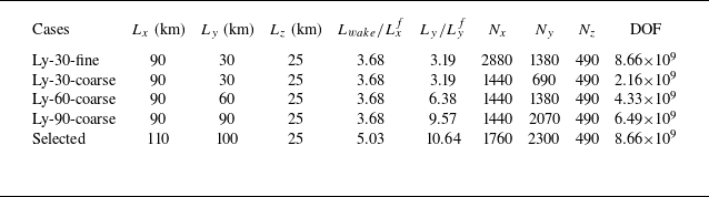
km. The wind farm is located in the main domain, which should be sufficiently large to avoid spurious effects introduced by the domain boundaries. In Appendix A, we analyse in detail the effects of the domain width on the wake evolution. Based on this analysis, we select a domain size
 $L_x \times L_y = 110 \times 100$
km
 $^2$
. Following previous studies, we fix the main domain height to
 $L_z=25$
km (Allaerts & Meyers Reference Allaerts and Meyers2017, Reference Allaerts and Meyers2018; Lanzilao & Meyers Reference Lanzilao and Meyers2022a
, Reference Lanzilao and Meyers2023, Reference Lanzilao and Meyers2024b
). Such a vertical extent allows gravity waves to decay and radiate energy outwards, therefore minimising reflectivity. A sketch of the main domain is reported in figure 2. We note that the precursor domain width and height should match those of the main domain when they are run concurrently. Therefore, after the precursor spin-up phase is completed, we extend the precursor flow fields in the
 $y$
direction from
 $10$
km to
 $100$
km by tiling together 10 copies of the same flow field. This is facilitated by the periodic boundary condition in the streamwise and spanwise directions. This technique has also been adopted by Sanchez Gomez et al. (Reference Sanchez Gomez, Lundquist, Mirocha and Arthur2023) and Lanzilao & Meyers (Reference Lanzilao and Meyers2024b
) for limiting the computational resources during the spin-up phase. Regarding the
 $z$
direction, the flow fields are extrapolated from
 $3$
km to
 $25$
km using a constant geostrophic wind. At these altitudes, the flow is laminar, and no turbulence is introduced. It is important to note that these operations are performed offline, meaning that they are carried out after the numerical solution has reached a statistically steady state within the precursor domain.
For the grid resolution, we fix
 $\Delta x = 62.5$
m and
 $\Delta y = 43.48$
m in the streamwise and spanwise directions, respectively. This leads to
 $N_x=1760$
and
 $N_y\,=\,2300$
grid points for the main domain, and to
 $N_x^p=160$
and
 $N_y^p=230$
points for the precursor domain. We note that the resolution adopted in this work is twice as coarse in both the streamwise and spanwise directions as that adopted in Lanzilao & Meyers (Reference Lanzilao and Meyers2022a
, Reference Lanzilao and Meyers2023, Reference Lanzilao and Meyers2024b
). This choice was dictated by the need for a sufficiently long and wide domain for studying the wake behaviour without spurious effects from the domain boundaries. We note that similar grid cell sizes have been used in other wind-farm wake studies (Baas & Verzijlbergh Reference Baas and Verzijlbergh2022; Maas & Raasch Reference Maas and Raasch2022; Baas et al. Reference Baas, Verzijlbergh, van Dorp and Jonker2023). Further, we also show in Appendix A that this change in grid resolution has very limited impact on the farm wake behaviour. In the vertical direction, we adopt a stretched grid that corresponds to that used in Lanzilao & Meyers (Reference Lanzilao and Meyers2022a
, Reference Lanzilao and Meyers2023, Reference Lanzilao and Meyers2024b
), i.e. with resolution
 $5$
m within the first
 $1.5$
km and stretched above, for a total of
 $490$
grid points. The combination of precursor and main domains leads to a total of approximately
 $8.65 \times 10^9$
degrees of freedom (DOF). We note that this number is evaluated as the product between the number of grid cells and the number of variables (i.e.
 $u$
,
 $v$
,
 $w$
and
 $\theta$
, which denote the streamwise, spanwise and vertical velocities, and the potential temperature field).
The top boundary conditions are a zero stress condition for the horizontal velocity, a zero vertical velocity, and a fixed potential temperature. Moreover, we use the Rayleigh damping layer (RDL), which extends from
 $15$
km to
 $25$
km. In this region, we add a body force in the momentum equations that dissipates the upward energy transported by gravity waves before it reaches the top of the domain, therefore minimising gravity-wave reflection. This is achieved by forcing the streamwise and spanwise velocity to the streamwise and spanwise components of the geostrophic wind, and by damping the vertical velocity (Allaerts & Meyers Reference Allaerts and Meyers2017; Lanzilao & Meyers Reference Lanzilao and Meyers2023). For the lower boundary condition, we employ a classic wall stress formulation based on the Monin–Obukhov similarity theory for neutral boundary layers (Moeng Reference Moeng1984; Allaerts & Meyers Reference Allaerts and Meyers2015). To avoid periodicity in the streamwise direction, we adopt the wave-free fringe-region technique developed by Lanzilao & Meyers (Reference Lanzilao and Meyers2023), located at the end of the main domain, starting at
 $x=104.5$
km and
 $5.5$
km long. In this region, we add a body force to the momentum equations that imposes the desired inflow conditions. Moreover, we damp the convection term in the vertical momentum equation to limit spurious gravity-wave effects. The location and dimension of the buffer regions are illustrated in figure 2. Moreover, the Rayleigh, damping and fringe functions adopted in this study are displayed in figure 3. We note that the set-up of these function parameters corresponds to that adopted by Lanzilao & Meyers (Reference Lanzilao and Meyers2024b
).
(a) Rayleigh function normalised with the Brunt–Väisälä frequency
 $N$
. The black horizontal dashed line denotes the start of the RDL, while the red dots denote the locations of the vertical grid cell centres. (b) Fringe and damping functions. The black vertical dashed line denotes the start of the fringe region, while the red vertical dashed line marks the end of the fringe forcing. The set-up of the Rayleigh, damping and fringe functions parameters corresponds to that adopted by Lanzilao & Meyers (Reference Lanzilao and Meyers2024b
).

2.3. Wind-farm set-up
The wind-farm layout and wind turbine choice correspond to those used previously by Lanzilao & Meyers (Reference Lanzilao and Meyers2022a
, Reference Lanzilao and Meyers2023, Reference Lanzilao and Meyers2024b
). Hence the farm has
 $16$
rows and
 $10$
columns, for a total of
 $160$
turbines. We adopt the 10 MW International Energy Agency offshore turbine, which has rotor diameter
 $D=198$
m and hub height
 $z_h=119$
m, leading to tip height
 $z_{{tip}}=218$
m (Bortolotti et al. Reference Bortolotti, Tarrés, Dykes, Merz, Sethuraman, Verelst and Zahle2019). Moreover, we fix the disk-based thrust coefficient
 $C_T'=1.94$
, which corresponds to
 $C_T=0.88$
. We remark that
 $C_T'$
represents the overall effect of blade lift and drag forces on the airflow at the rotor disk, non-dimensionalised with the velocity measured at the rotor disk (Calaf et al. Reference Calaf, Meneveau and Meyers2010). The turbines are arranged in a staggered layout with respect to the main wind direction, with streamwise and spanwise spacings set to
 $S_x=S_y=5D$
, resulting in farm length and width
 $L_x^f=14.85$
km and
 $L_y^f=9.4$
km, respectively. Moreover, a simple yaw controller is implemented to keep the turbine-rotor disks perpendicular to the incident wind flow measured one rotor diameter upstream. The first row of turbines is located
 $15$
km from the inflow, while the distance between the last row and the start of the fringe region amounts to approximately
 $75$
km. We selected this configuration to enable the full development of the wind-farm wake, thereby facilitating a detailed examination of the mechanisms involved in the wake recovery. Moreover, the ratio
 $L_y/L_y^f$
measures
 $10.64$
, which is well in line with the guidelines proposed by Lanzilao & Meyers (Reference Lanzilao and Meyers2024b
). The main domain sketch reported in figure 2 further illustrates the wind-farm location and its size relative to the computational domain.
2.4. Atmospheric state
The initial atmospheric states are chosen based on the analysis performed in Lanzilao & Meyers (Reference Lanzilao and Meyers2024b
). Hence we fix the geostrophic wind to
 $G=10$
m s
 $^{-1}$
, so that all turbines operate below their rated power and in a region where the thrust curve typically shows a rather constant thrust coefficient value. In regard to the capping-inversion height
 $H$
, we initialise its value to
 $150$
,
 $300$
,
 $500$
and
 $1000$
m. This allows us to explore farm operations in shallow and deep boundary layers. The capping inversion strength
 $\Delta \theta$
is set to
 $5$
K, while we fix the free-atmosphere lapse rate
 $\Gamma$
to
 $4$
K km
 $^{-1}$
. Further, the ground temperature and the capping-inversion thickness are fixed to
 $\theta _0=288.15$
K and
 $\Delta H = 100$
m for all simulations. Finally, we select latitude
 $\phi =51.6^\circ$
, which leads to Coriolis frequency
 $f_c=1.14 \times 10^{-4}$
s
 $^{-1}$
and surface roughness
 $z_0 = 1 \times 10^{-4}$
m. This value represents calm sea conditions and is in the range of values observed over the North Sea, and more generally offshore (Taylor & Yelland Reference Taylor and Yelland2000; Allaerts & Meyers Reference Allaerts and Meyers2017; Kirby, Nishino & Dunstan Reference Kirby, Nishino and Dunstan2022; Lanzilao & Meyers Reference Lanzilao and Meyers2022a
). Since the only changing parameter among the four cases considered is the capping inversion height, we denote these cases as H150, H300, H500 and H1000. We note that during the spin-up phase of the precursor, the value of the capping-inversion height slightly grows – see § 3.1.
In the remainder of the text, the state variables will be accompanied by a bar in case of time averages. For the horizontal averages along the full streamwise and spanwise directions, we use angular brackets
 $\langle \cdot \rangle$
, while the notations
 $\langle \cdot \rangle _{\!f}$
and
 $\langle \cdot \rangle _{\!w}$
are used to represent spanwise averages along the farm and wake widths, respectively. Finally, we note that the RDL and fringe region will be left out of the figures in the remainder of the text.
3. Boundary-layer initialisation
In this section, we summarise the methodology applied to spin-up the precursor and wind-farm simulations. We note that the methodology follows that adopted by Lanzilao & Meyers (Reference Lanzilao and Meyers2024b ). Therefore, we refer the reader to their work for more details.
3.1. Generation of a fully developed turbulent flow field
The initial vertical potential temperature profiles are generated giving the
 $H$
,
 $\Delta H$
,
 $\Delta \theta$
and
 $\Gamma$
values as input to the Rampanelli & Zardi (Reference Rampanelli and Zardi2004) model. For the initial velocity profile, we use a constant geostrophic wind above the capping inversion. Within the ABL, we use the Zilitinkevich (Reference Zilitinkevich1989) model with friction velocity
 $u_\ast = 0.26$
m s
 $^{-1}$
, which is in the range of values observed by Brost, Lenschow & Wyngaard (Reference Brost, Lenschow and Wyngaard1982). The velocity profiles below the capping inversion are then combined with the laminar profile in the free atmosphere following the method proposed by Allaerts & Meyers (Reference Allaerts and Meyers2015).
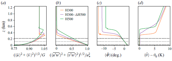
Vertical profiles of (a) velocity magnitude, (b) total shear stress magnitude, (c) wind direction and (d) potential temperature averaged along the full horizontal directions and over the last
 $4$
h of the simulation. The continuous lines denote the profiles used in this work, while the dashed lines represent the profiles obtained with a finer horizontal grid resolution with
 $\Delta x/2$
and
 $\Delta y/2$
(i.e. the profiles used by Lanzilao & Meyers Reference Lanzilao and Meyers2024b
). The grey dashed line denotes the turbine-hub height, while the black dashed lines are representative of the rotor dimension. We note that the results shown here only refer to the precursor simulations.

Next, we add random divergence-free perturbations with amplitude
 $0.1G$
in the first
 $100$
m to the vertical velocity profiles. This initial state is given as input to the precursor simulation. The flow is advanced in time for
 $20$
h, which is sufficient to obtain a turbulent fully developed statistically steady state (Pedersen, Gryning & Kelly Reference Pedersen, Gryning and Kelly2014; Allaerts & Meyers Reference Allaerts and Meyers2017; Lanzilao & Meyers Reference Lanzilao and Meyers2023, Reference Lanzilao and Meyers2024b
). Figure 4 illustrates vertical profiles of several quantities of interest averaged over the last
 $4$
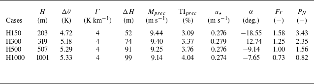
h of the simulations and over the full horizontal directions. Figure 4(a) shows the velocity magnitude normalised with the geostrophic wind. The boundary layer extends up to the capping inversion, which limits its growth. All velocity profiles show a common feature, i.e. the presence of a super-geostrophic jet near the top of the ABL, which is a typical phenomenon observed in this type of atmospheric conditions (Pedersen et al. Reference Pedersen, Gryning and Kelly2014; Allaerts & Meyers Reference Allaerts and Meyers2015; Goit & Meyers Reference Goit and Meyers2015). Such a jet is more accentuated for the H150 cases, where a stronger wind shear within the ABL is attained. Next, figure 4(b) displays the sum of the modelled and resolved shear stress magnitude, which is non-zero only below the capping inversion, with a quasi-linear profile. Further, figure 4(c) shows the flow angle. At turbine-hub height, the flow is parallel to the
 $x$
direction. This is achieved by using the wind-angle controller developed and tuned by Allaerts & Meyers (Reference Allaerts and Meyers2015), which is designed to ensure a desired orientation of the hub-height wind direction (
 $\Phi _d =0^\circ$
in this case). We also observe that most of the wind-direction change occurs within the inversion layer, except for case H1000. The geostrophic wind angle, which is the angle between the surface stress and the geostrophic wind velocity, is larger for shallow boundary layers, as noted by Allaerts & Meyers (Reference Allaerts and Meyers2017), going from
 $-18.55^\circ$
to
 $-7.65^\circ$
in cases H150 and H1000, respectively. Finally, the thermal stratification is illustrated in figure 4(d) by means of potential temperature profiles. For the sake of completeness, we also show the profiles obtained on a finer grid resolution – i.e. the one adopted by Lanzilao & Meyers (Reference Lanzilao and Meyers2024b
). Figure 4 shows that doubling the grid cell size in the streamwise and spanwise directions has negligible effects on the precursor results, particularly in the region where the turbines are located – see Appendix A for more details. The four spin-up cases together with some parameters of interest averaged over the last
 $4$
h of simulation are summarised in table 1.
Overview of the spin-up cases used to drive the wind-farm simulations. The parameters are averaged over the last 4 h of the spin-up phase, and include the capping-inversion height
 $H$
, the capping-inversion strength
 $\Delta \theta$
, the free atmosphere lapse rate
 $\Gamma$
, the capping-inversion thickness
 $\Delta H$
, the velocity magnitude measure at hub height
 $M_{{prec}}=(\langle \bar {u} \rangle ^2 + \langle \bar {v} \rangle ^2 )^{1/2}$
, the turbulence intensity measured at hub height
 $\mathrm{TI}_{{prec}}=(2e_{{prec}}/3M_{{prec}}^2)^{1/2}$
with
 $e_{{prec}}$
the TKE, the friction velocity
 $u_\star$
, the geostrophic wind angle
 $\alpha$
, the Froude number Fr and the
 $P_N$
number. Note that the parameters
 $H$
,
 $\Delta \theta$
,
 $\Gamma$
and
 $\Delta H$
have been estimated by fitting the spin-up profiles averaged over the last 4 h of the precursor simulations with the Rampanelli & Zardi (Reference Rampanelli and Zardi2004) model.

The four spin-up cases together with some parameters of interest averaged over the last
 $4$
h of simulation are summarised in table 1. We remark that the capping-inversion height moves upwards during the spin-up phase, particularly for the shallow-boundary-layer cases. For instance, the H150 cases show a growth of
 $53$
m on average over the
 $20$
h of spin-up. Moreover, the capping-inversion strength and thickness also reduce, down to
 $4.72$
K and
 $52$
m, respectively. For the H1000 cases, the vertical potential temperature profile shows only very minor changes from its initial state. As a result of these changes, it is important to note that cases H150, H300, H500 and H1000 have effective capping-inversion heights
 $203$
,
 $319$
,
 $507$
and
 $1001$
m.
3.2. Wind-farm start-up phase
The four precursor fields discussed previously are now used to drive four simulations in the main domain, where the wind farm actively imposes a drag force on the flow. However, before collecting flow statistics over time, a second spin-up phase is required. In fact, the flow has to adjust to the presence of the farm in the main domain before reaching a new statistically steady state. Lanzilao & Meyers (Reference Lanzilao and Meyers2024b
) have shown that 1 h of wind-farm spin-up time suffices for the flow to adjust to the farm drag force. However, the domain length adopted in this work is more than twice that used by Lanzilao & Meyers (Reference Lanzilao and Meyers2024b
). Hence we fix the duration of the wind-farm start-up phase to
 $5.5$
hours, which corresponds to approximately 12 and 1.7 wind-farm and domain flow-through times, respectively. Next, we switch off the wind-angle controller in the precursor domain, and we collect statistics during a 2 h time window.
4. Results
The sensitivity of the flow blockage and wind-farm performance to the thermal stratification above the ABL have been already analysed in detail by Lanzilao & Meyers (Reference Lanzilao and Meyers2024b
), who adopted the same wind farm used in this study. Therefore, the focus of this section is solely on the wake properties and its recovery mechanisms as the height of the capping inversion varies. We recognise that other parameters that define the thermal stratification above the ABL may also have an influence on the wake behaviour. An example is discussed in Appendix B, where we vary the capping-inversion thickness
 $\Delta h$
from 100 m to 500 m. Here, § 4.1 presents a qualitative analysis of the wake behaviour when
 $H$
varies. In § 4.2, we perform a quantitative analysis by introducing a simple fitting model for inferring quantities such as the wake strength, deflection and width along the streamwise direction, together with characterising the vertical and horizontal wake development. Finally, a streamwise and spanwise momentum budget analysis is performed in § 4.3 and § 4.4, respectively, where we discuss in detail the dominant terms that replenish the wind-farm wake. We remark that the results shown in the remainder of the text are time-averaged over the last
 $2$
h of simulation time. Further, given tip height
 $218$
m, we will often refer to cases H150 and H300 as shallow-boundary-layer cases, while H500 and H1000 will often be denoted as deep-boundary-layer cases.
4.1. Flow physics
We start our analysis with figure 5, which shows a side view of turbulent kinetic energy (TKE) perturbation with respect to the precursor simulation averaged in the
 $y$
direction along the width of the farm, together with the base and top of the inversion layer computed by fitting the LES data with the Rampanelli & Zardi (Reference Rampanelli and Zardi2004) model. In the H150 and H300 cases, the vicinity of the capping inversion to the turbine-tip height limits the flow development in the vertical direction. Moreover, the capping inversion behaves as a pliant surface, limiting flow entrainment from the free atmosphere. Further, the high stability attained within the inversion layer dampens turbulence, therefore severely limiting the vertical development of the internal boundary layer. Consequently, figure 5(a,b) display relatively high values of TKE only within the farm, which then decay downwind of the last row of turbines. Moreover, the very low vertical mixing of momentum due to the vicinity of the inversion layer significantly reduces the wind shear at hub height in the wake region (see also figure 6
a), which further causes the TKE to drop below the values attained in the precursor simulations. The combination of these effects leads to very strong velocity deficit in the farm wake and a slow recovery rate, as shown in figure 6(a,b). The increase in the
 $H/z_{{tip}}$
ratio for cases H500 and H1000 allows for higher TKE values and accounts for a significant vertical development of the internal boundary layer, as shown in figure 5(c,d). The latter enhance vertical turbulent transport of momentum, therefore giving rise to lower wake deficit and a faster recovery rate, as visible in figure 6(c,d). Moreover, case H1000 shows the formation of a high speed channel between the tip height and the capping-inversion base, which further increases the TKE and flow mixing. Stieren & Stevens (Reference Stieren and Stevens2022) mentioned that a wind farm operating in the wake of an upstream one is negatively affected in terms of power output, but has a higher wake efficiency due to the increased turbulence level in the incoming inflow. Figure 5 shows that this is the case only in deep boundary layers and only when the farm is less distant than
 $10$
–
 $20$
km, as the TKE decays much faster than the velocity deficit. The latter, shown in figure 6, illustrates that the wake is not fully replenished in all cases, meaning that it would impact on downwind farms located more than
 $70$
km downstream. Finally, above the inversion layer, the internal gravity waves generate a slanted pattern of alternating positive and negative perturbations in all fields (Allaerts & Meyers Reference Allaerts and Meyers2017). The phase of these perturbations in each field is governed by the polarisation equation, which is derived from linear gravity-wave theory (Nappo Reference Nappo2002). This equation shows that the perturbations in the streamwise velocity component are out of phase with respect to the pressure perturbation (see Lanzilao & Meyers (Reference Lanzilao and Meyers2024b
) Appendix C for a simplified derivation). Since internal waves generate a negative pressure perturbation in the free atmosphere and downstream of the maximum capping-inversion displacement (i.e. above the farm), this results in a flow speed-up in the same region, particularly accentuated in shallow-boundary-layer cases.
Contours of the time-averaged TKE perturbation with respect to the precursor simulation taken in an
 $x$
–
 $z$
plane further averaged along the farm width in the spanwise direction for cases (a) H150, (b) H300, (c) H500 and (d) H1000. The black lines represent the bottom and top of the inversion layer computed with the Rampanelli & Zardi (Reference Rampanelli and Zardi2004) model. The locations of the turbine-rotor disks are indicated with vertical white lines.

Contours of the time-averaged horizontal velocity magnitude in an
 $x$
–
 $z$
plane further averaged along the farm width in the spanwise direction for cases (a) H150, (b) H300, (c) H500 and (d) H1000. The black lines represent the bottom and top of the inversion layer computed with the Rampanelli & Zardi (Reference Rampanelli and Zardi2004) model. The locations of the turbine-rotor disks are indicated with vertical white lines.

Contours of the time-averaged (a–d) horizontal velocity magnitude, (e–h) flow angle, (i–l) vertical velocity, (m–p) pressure perturbation with respect to the inflow, and (q–t) TKE perturbation with respect to the precursor simulation in an
 $x$
–
 $y$
plane, taken at hub height for cases (a,e,i,m,q) H150, (b,f,j,n,r) H300, (c,g,k,o,s) H500 and (d,h,l,p,t) H1000. The location of the wind farm is indicated with the black rectangle. The last 10 km of domain in the streamwise direction are not displayed as the solution is influenced by the fringe forcing in that region.

Next, figure 7(a–d) show a top view taken at hub height of horizontal velocity magnitude. First, we observe that in all cases, the velocity deficit does not seem to spread horizontally. A similar behaviour can be observed in numerical simulations and SAR images, such as figure 1 (Baas & Verzijlbergh Reference Baas and Verzijlbergh2022; Maas & Raasch Reference Maas and Raasch2022; Finserås et al. Reference Finserås, Herrera Anchustegui, Cheynet, Gebhardt and Reuder2024). Therefore, the assumption that the velocity deficit spreads linearly, which is typically made in analytical wake models, seems to not hold for wind-farm wakes. As shown previously, the vicinity of the capping inversion to turbine-tip height in cases H150 and H300 limits the flow development in the vertical direction. Therefore, to conserve mass, high-speed regions form at the sides of the wake. The same phenomenon was also observed by Lanzilao & Meyers (Reference Lanzilao and Meyers2024b ). The strong flow deceleration attained in these two cases decreases the Coriolis force magnitude, which scales linearly with the wind speed. Hence the wake turns towards the direction of the background pressure gradient, therefore undergoing an anticlockwise flow rotation.
In the H500 and H1000 cases, the wake recovery rate is higher, enhanced by the vertical turbulent entrainment of momentum. The latter adds clockwise-turning flow from aloft into the wake region. Therefore, a clockwise wake deflection is observed, which is dictated by the wind veer present in the background flow. This behaviour is also illustrated in figure 7(e–h), which display the flow angle at hub height. These plots clearly show that effects of Coriolis forces and wind veer are opposed. Whether one dominates the other depends upon the capping-inversion height. Moreover, we can also conclude that in the absence of wind veer in the background flow, the wind-farm wake would be always deflected anticlockwise in the northern hemisphere. We note that similar results have been observed for both single-turbine and wind-farm wake simulations (van der Laan & Sørensen Reference van der Laan and Sørensen2017; Howland, Ghate & Lele Reference Howland, Ghate and Lele2018; Heck & Howland Reference Heck and Howland2025). The typical signature of trapped waves is visible in the vertical velocity field shown in figure 7(i–l), particularly in the shallow-boundary-layer cases where the capping inversion is closer to hub height. The V-shaped pattern attained in sub-critical flows, also visible in the pressure perturbation fields shown in figure 7(m–p), has been already observed and analysed in detail by Allaerts & Meyers (Reference Allaerts and Meyers2019) and Lanzilao & Meyers (Reference Lanzilao and Meyers2024b
). However, we notice the presence of slanted waves with a high wavenumber that cross the full domain in the streamwise direction, particularly visible in cases H150 and H300. The same behaviour has been observed by Lanzilao & Meyers (Reference Lanzilao and Meyers2024b
), who showed that these slanted waves originate from the perturbation introduced by the turbine spacing, and their angle with respect to the
 $x$
-axis can be predicted with linear theory for deep-water waves. We refer the reader to Lanzilao & Meyers (Reference Lanzilao and Meyers2024b
) for more details. Finally, we note in figure 7(i,j) the presence of a region of positive vertical velocity on the left edge of the wake. This denotes a region of flow convergence, which will be discussed later in this section. To conclude, figure 7(q–t) illustrate the TKE perturbation with respect to the precursor simulation at hub height. As expected, a higher TKE level is obtained in deeper boundary layers. For shallow boundary layers, the TKE at hub height in the wake of the farm is smaller than the precursor value, as also shown in figure 5(a,b). This is a consequence of the reduced velocity shear in the farm wake in the region below
 $H$
, which therefore diminishes the production of turbulence. Similar results have been observed in wind tunnel experiments and mesoscale models (Chamorro & Porté-Agel Reference Chamorro and Porté-Agel2009; Fitch et al. Reference Fitch, Olson, Lundquist, Dudhia, Gupta, Michalakes and Barstad2012). Similar to Maas (Reference Maas2023b
), we notice a higher level of TKE on the left side of the wake, i.e. at
 $y=55$
km.
Contours of the time-averaged streamwise velocity in an
 $y$
–
 $z$
plane focused on the wake region and its sides taken at (a)
 $x=50$
km, (b)
 $x=70$
km and (c)
 $x=100$
km for case H300. The arrows represent the in-plane velocity vector given by the spanwise and vertical velocity components. The vector is normalised with its magnitude
 $(\bar {v}^2+\bar {w}^2)^{1/2}$
, so that all arrows have the same length. The blue lines represent the bottom and top of the inversion layer computed with the Rampanelli & Zardi (Reference Rampanelli and Zardi2004) model. The vertical black dashed lines denote the centreline of the mixing layers located at the sides of the wake – see the fitting model introduced in § 4.2.

Next, we investigate the flow behaviour in the wake region and at its sides. To do so, we illustrate
 $y$
–
 $z$
planes of streamwise velocity taken at
 $x=50$
,
 $70$
and
 $100$
km for case H300 in figure 8. Moreover, we add vectors that denote the flow direction based on the spanwise and vertical velocity components, while their colours indicate the in-plane velocity magnitude (i.e.
 $(\bar {v}^2+\bar {w}^2)^{1/2}$
). Further, we remark that due to the convention used, the right side of the wake corresponds to the left side of the figure, and vice versa – see figure 2.
At
 $x=50$
km (i.e.
 $20$
km downstream of the farm), figure 8(a) shows a strong streamwise velocity deficit, which spreads over the whole ABL height. Within the wake and on its right side, the flow direction follows the wind veer profile of the background flow (i.e. a positive and negative spanwise velocity below and above turbine-hub height). However, the zero flow-angle height is shifted upwards, close to turbine-tip height. This is a consequence of the reduced Coriolis force and absence of vertical mixing, which causes the flow to turn towards the background pressure gradient. Moreover, we observe the presence of anticlockwise flow recirculation within the wake region, induced by the trapped waves that also corrugate the base and top of the capping inversion. The flow near the left edge of the wake behaves differently. Here, we observe an anticlockwise motion of the wake, with a positive spanwise component below tip height, an upward motion at the wake edge, and a negative spanwise component near the base of the capping inversion. As a result, the spanwise velocity component attains values close to zero at this edge (i.e. at
 $y\approx 56$
km), significantly limiting the advection of mean flow – see § 4.3. On the left side, we observe the presence of trapped waves which leads to an anticlockwise flow motion.
Figure 8(b,c) show the flow behaviour at
 $x=70$
km and
 $x=100$
km, respectively. As we move downstream, the streamwise velocity component recovers at a slow rate along the downstream direction, while the wake gradually narrows. The zero flow-angle height moves downwards towards turbine-hub height, with the wind veer profile converging towards that of the background flow within the wake and on its right side. However, the anticlockwise motion at the left edge of the wake does not die out and is still clearly visible
 $50$
km downstream of the farm. Contrarily, the trapped waves at the left side of the wake are gradually dampened along the streamwise direction, so that the anticlockwise flow rotation at the left side of the wake vanishes at
 $x=100$
km, and the flow assumes a negative spanwise component at each height. Finally, figure 8(b,c) also illustrate how the strong wind veer attained on the right edge of the wake causes the streamwise velocity deficit to spread horizontally.
Contours of the time-averaged streamwise velocity in an
 $y$
–
 $z$
plane focused on the wake region and its sides taken at (a)
 $x=50$
km, (b)
 $x=70$
km and (c)
 $x=100$
km for case H1000. The arrows represent the in-plane velocity vector given by the spanwise and vertical velocity components. The vector is normalised with its magnitude
 $(\bar {v}^2+\bar {w}^2)^{1/2}$
, so that all arrows have the same length. The vertical black dashed lines denote the centreline of the mixing layers located at the sides of the wake – see the fitting model introduced in § 4.2.

The same analysis for case H1000 is shown in figure 9. Here, the flow behaviour is significantly different from that obtained in shallow boundary layers. In fact, the strong flow mixing along the vertical direction adds clockwise-turning flow from aloft into the wake region. Consequently, figure 9(a) illustrates that the streamwise velocity deficit recovers at a much faster rate, with the spanwise velocity component being negative at each height within the wake region. Moreover, the wind veer is significantly reduced if compared to that of the background flow. Further, we also observe a much stronger in-plane velocity magnitude compared to case H300. At the sides of the wake, the wind veer follows the same orientation as that attained within the wake region. Moreover, flow recirculation induced by trapped waves remains very limited. In fact, the influence of trapped waves on the flow behaviour within the rotor height is very limited in deep boundary layers – see figure 7(l). Further downstream, figure 9(b,c) show that the streamwise velocity deficit is mostly recovered and the wake deflects clockwise. Moreover, the streamwise velocity deficit does not spread along the horizontal direction as a consequence of the reduced wind veer.
4.2. Wake properties
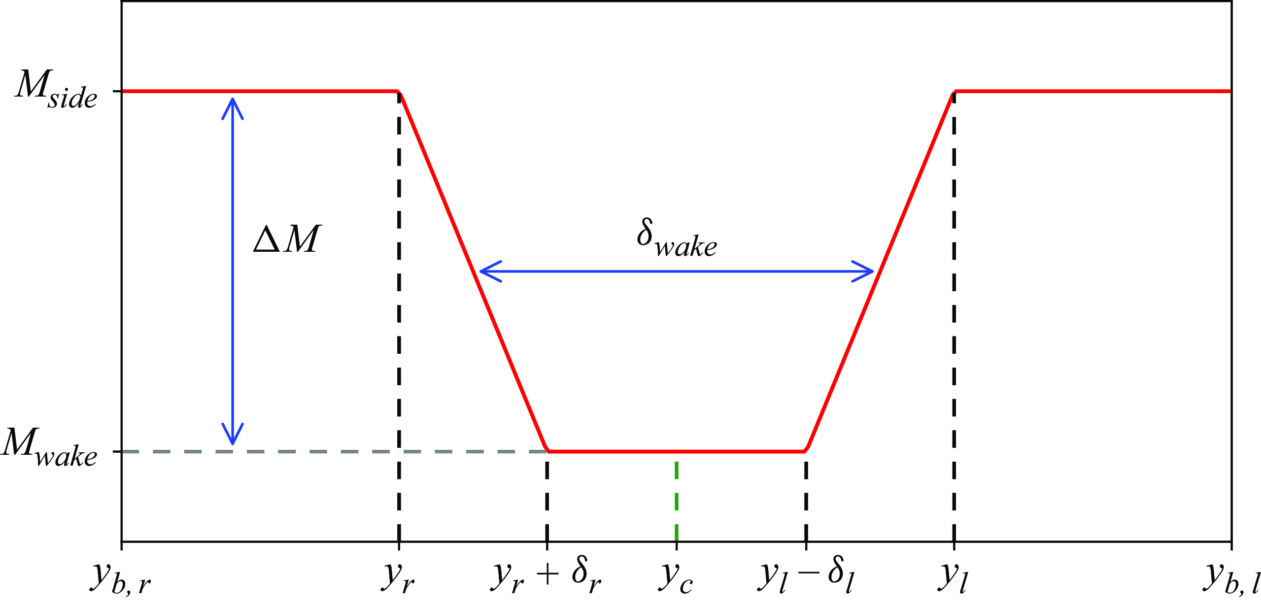
We have seen in the previous subsection that the wake region is heavily dependent upon the capping-inversion height. In this subsection, we will investigate the vertical and horizontal wake development. Moreover, we will rigorously define the wake edges and centre, which we use to evaluate the wake width, strength and deflection. To do so, we propose a simple function that we use to fit the velocity magnitude profiles along the spanwise direction:
 \begin{equation} F(y) = \begin{cases} M_{{side}}& \text{if } y_{b,r} \leqslant y \lt y_r,\\ M_{{side}} - \Delta M (y-y_r)/\delta _r & \text{if } y_r \leqslant y \lt y_r + \delta _r, \\ M_{{wake}} & \text{if } y_r + \delta _r \leqslant y \lt y_l - \delta _l, \\ M_{{wake}} + \Delta M (y-y_l+\delta _l)/\delta _l& \text{if } y_l - \delta _l \leqslant y \lt y_l, \\ M_{{side}}& \text{if } y_l \leqslant y \lt y_{b,l}, \end{cases} \end{equation}
where
 $M_{{side}}$
and
 $M_{{wake}}$
denote the velocity magnitudes attained at the sides and in the wake of the farm, while
 $y_r$
and
 $y_l$
denote the right- and left wake-edge locations, located in the region around
 $y=45$
km and
 $y=55$
km, respectively. We remark that due to the convention used, the right side of the wake corresponds to the left side of the figure, and vice versa. Moreover, we note that the velocity
 $M_{{side}}$
is measured in a region that extends
 $10$
km sideways of the farm location, so that its value does not depend upon the spanwise domain dimension. Hence
 $y_{b,r}$
and
 $y_{b,l}$
assume values
 $35$
km and
 $65$
km, respectively. Further,
 $\delta _r$
and
 $\delta _l$
represent the distances over which the velocity decays from
 $M_{{side}}$
to
 $M_{{wake}}$
. Further,
 $\Delta M = M_{{side}} - M_{{wake}}$
indicates the velocity deficit with respect to the wind speed at the wake sides. Note that this is also the definition of velocity deficit typically used in real case scenarios (Djath et al. Reference Djath, Schulz-Stellenfleth and Cañadillas2018). Following Pope (Reference Pope2000), we define the farm wake width as the distance between the centreline of the regions
 $\delta _l$
and
 $\delta _r$
, i.e.
 $\delta _{{wake}} = y_l - \delta _l/2 - (y_r + \delta _r/2)$
. Further, we define the wake centre as the middle point of the region where
 $M_{{wake}}$
is attained, which is formally defined as
 $y_c=(y_l-\delta _l+y_r+\delta _r)/2$
. The fitting function
 $F(y)$
reported in (4.1) together with a visual representation of its parameters is shown in figure 10.
Sketch of the fitting function
 $F(y)$
and its parameters – see (4.1).

Time-averaged horizontal velocity magnitude as a function of the spanwise direction obtained at
 $x=x_0$
(brightest yellow) and
 $x=x_0+70$
(darkest blue), with increments of
 $5$
km in between, for cases (a) H150, (b) H300, (c) H500 and (d) H1000. Each symbol denotes a spanwise average over one turbine spacing (i.e.
 $5D$
). The red dashed lines illustrate the results of our fitting model for each streamwise location. The vertical dashed black lines denote the location of the first- and last-column turbines. We define the regions around
 $y=45$
km and
 $y=55$
km as the right- and left edges, respectively, and
 $x_0=30$
km denotes the beginning of the wake region.

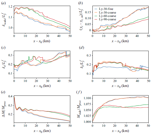
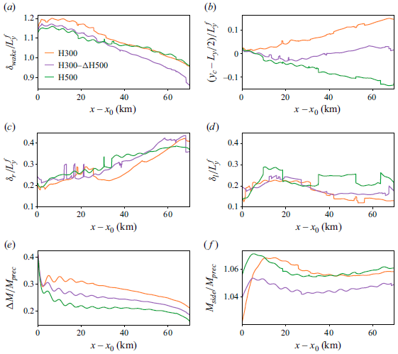
(a,b) Wake width, wake centre and (c,d) right- and left mixing layer widths normalised with the farm width. (e,f) Velocity deficit with respect to
 $M_{{side}}$
, and velocity magnitude at the sides of the wake, normalised with the velocity magnitude obtained in the precursor domain at hub height. All quantities are predicted by the fitting model shown in (4.1). The
 $x$
-axis is rescaled with
 $x_0=30$
km, which denotes the beginning of the wake region.

The only purpose of the model reported in (4.1) is to identify the wake location and shape in a horizontal plane given a velocity profile along a direction normal to the farm wake. The profiles obtained for this study are shown in figure 11 at various locations downwind of the farm (i.e. from
 $x=x_0$
to
 $x=x_0+70$
with increments of
 $5$
km). figure 11(a,b) show the profiles for cases H150 and H300. Here, we can observe strong velocity deficits within the first
 $10$
km, where the profiles assume a top-hat shape with peaks in the location of the first and last column of turbines. This behaviour may be caused by the strong flow redirection at the farm sides, which yaws the first and last columns of turbines up to 8
 $^\circ$
in case H150, allowing for a higher energy extraction and therefore causing higher velocity deficit at
 $y=45$
km and
 $y=55$
km (Lanzilao & Meyers Reference Lanzilao and Meyers2024b
). In these cases, the wake turns anticlockwise. Therefore, the velocity gradient within the right edge of the wake (i.e. at
 $y=45$
km) diminishes along the streamwise direction. Moreover, the vertical velocity profiles at the lateral edges of the wake are only slightly dependent on the vertical direction for
 $z\lt H$
and the ratio
 $\delta _{{wake}}/H \gg 1$
– see figure 12(a). Consequently, the regions
 $\delta _l$
and
 $\delta _r$
can be interpreted as two distinct mixing layers with width varying along the streamwise direction. In figure 11(a,b), we observe that the mixing layer located at the right edge of the wake expands along the streamwise direction, with its centreline turning towards the low-velocity side. On the contrary, the mixing layer on the left edge of the wake (i.e. at
 $y=55$
km) has a limited growth, possibly due to the fact that the wake turns in the direction opposite to the wind veer of the background flow. Next, figure 11(c,d) show the results for the deep-boundary-layer cases, i.e. H500 and H1000. The velocity profiles fully resemble a top-hat shape with smooth edges. The wake turns clockwise in these cases, and the velocity speed-up at the wake sides is less pronounced. Finally, for case H1000, with
 $\delta _{{wake}}/H \approx 10$
, we find that the mixing layer analogy no longer works, with velocity profiles that depend significantly on height (see figure 15), and wake recovery that is dominated by vertical entrainment – see § 4.3. The velocity magnitude profiles discussed above are then fitted using the model reported in (4.1). The fitting is performed using the curve_fit method provided by the Scipy library, adopting the trust region reflective algorithm (Virtanen et al. Reference Virtanen2020). The results are shown in figure 11, where the red dashed lines illustrate the fitted velocity profiles. Here, we can observe that the model captures the wake location and strength very well.
The wake width and centre, the velocity deficit and the velocity at the wake sides, together with the mixing layers width, all evaluated at hub height and estimated using the fitting model reported in (4.1), are shown in figure 12. The wake width, which is defined as the distance between the left- and right mixing layers, is shown in figure 12(a). Here, we can observe a width
 $10$
–
 $20$
% higher than
 $L_y^f$
at the beginning of the wake region. Further downstream, the mixing layer centrelines turn towards the low-velocity side, resulting in a reduction of
 $\delta _{{wake}}$
. At
 $x-x_0=65$
km, cases H150, H300 and H500 show a wake-to-farm width ratio of roughly 1, while case H1000 displays a narrower wake. The wake narrowing along the streamwise direction can also be observed in SAR images and in the results shown by Baas & Verzijlbergh (Reference Baas and Verzijlbergh2022), Maas & Raasch (Reference Maas and Raasch2022) and Baas et al. (Reference Baas, Verzijlbergh, van Dorp and Jonker2023). In particular, Maas (Reference Maas2023b
) performed a wind-farm simulation with inflow conditions similar to our H300 case, and observed very similar trends in both wake width and deflection. The wake centre is displayed in figure 12(b). Here, we observe how the capping-inversion height influences the wake deflection, generating a clear distinction between shallow and deep boundary layers. The strongest wake deflection is observed in case H1000, where the wake centre deviates by approximately
 $45$
% of the wake width
 $65$
km downstream of the farm. Next, figure 12(c,d) show the widths of the regions at the side of the farm over which the velocity decays from
 $M_{{side}}$
to
 $M_{{wake}}$
. The region
 $\delta _r$
becomes three times wider while going from
 $x_0$
km to
 $x_0+70$
km in the H150 case, while it shows a more limited growth in the other cases. Except for case H1000, this growth can be interpreted as an expanding mixing layer along the streamwise direction. On the left side, the region
 $\delta _l$
preserves approximately its width, as illustrated in figure 12(d). A growth is observed only in the H1000 cases, although it happens mostly within the first
 $10$
km downwind of the farm. These behaviours can also be observed in figure 11.
Next, figure 12(e) illustrates the velocity deficit with respect to the velocity measured at the sides of the wake and further normalised with the precursor velocity at hub height. In all cases, the wake shows a very fast recovery rate within the first
 $5$
km. Afterwards, the velocity deficit attains a very slow recovery, except for case H1000 where
 $\Delta M$
keeps decreasing up to
 $40$
km downwind of the farm. We note that the ratio
 $\Delta M/M_{{prec}}$
measures approximately
 $0.25$
at the end of the wake region in cases H150 and H300, confirming that the wake is not replenished. Moreover, we remark the presence of oscillations in the
 $\Delta M$
profiles with decreasing amplitude for increasing values of
 $H$
. These oscillations are related to the flow divergence–convergence generated by interfacial waves (see figure 7
i–l), and therefore are more accentuated in shallow boundary layers. Figure 12(f) shows the velocity at the sides of the wake normalised with
 $M_{{prec}}$
. Lanzilao & Meyers (Reference Lanzilao and Meyers2024b
) have shown that shallow boundary layers cause the flow to speed up at the farm sides. The same phenomenon is visible here. For instance, in case H150,
 $M_{{side}}/M_{{prec}}$
goes from
 $0.99$
to
 $1.07$
in the first
 $20$
km downwind of the farm. A high capping inversion allows the internal boundary layer to grow vertically, resulting in lower
 $M_{{side}}/M_{{prec}}$
ratios. We also note that the maximum
 $M_{{side}}/M_{{prec}}$
value shifts downstream as
 $H$
decreases.
Mixing layers centreline and wake centre measured at
 $z_h-D/2$
,
 $z_h$
and
 $z_h+D/2$
for cases (a) H150, (b) H300, (c) H500 and (d) H1000 predicted by the fitting model shown in (4.1). The black horizontal dashed lines denote the locations of the first and last turbine columns. The
 $x$
-axis is rescaled with
 $x_0=30$
km, which denotes the beginning of the wake region.

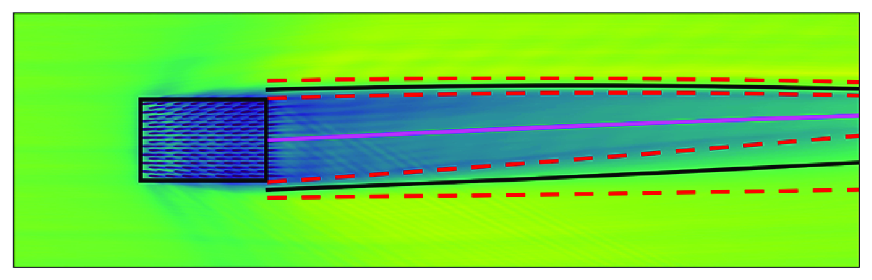
Contours of the time-averaged horizontal velocity magnitude downwind of the farm for cases (a) H150, (b) H300, (c) H500 and (d) H1000 in an
 $x$
–
 $y$
plane taken at hub height. The black lines denote the centreline of the mixing layers, while the red dashed lines denote their width. The pink line indicates the wake centre. All quantities are predicted by the fitting model shown in (4.1). The
 $x$
-axis is rescaled with
 $x_0=30$
km, which denotes the beginning of the wake region.

Up to this point, we have investigated only the wake properties at hub height. Looking at the wake evolution at different heights, figure 13 shows the centreline of the mixing layers
 $y_r+\delta _r/2$
and
 $y_l-\delta _l/2$
together with the wake centre at the heights
 $z_h-D/2$
,
 $z_h$
and
 $z_h+D/2$
, for all cases. While the wake turns anticlockwise at hub height for case H150, we can observe a strong clockwise rotation of the velocity deficit at tip height. This effect is caused by the strong wind veer attained within the capping inversion, which is very near to tip height in this case. Moreover, the noise observed in the blue lines around
 $x=90$
km is due to the vicinity of the capping inversion, where the velocity deficit assumes a different profile than the one that our model can fit. In all other cases, the wake edges and centre do not differ substantially across the rotor height. Moreover, we also note that the wake recovery rate does not vary across the rotor height (not shown).
Next, we apply a quadratic fit along the streamwise direction to the profiles obtained with the fitting model in order to average out small oscillations, and we superimpose them to the hub-height horizontal velocity magnitude field. The results for all cases are shown in figure 14. Here, we can observe that we correctly track the wake evolution along the streamwise direction. Moreover, we can observe the evolution of the mixing layers width at the sides of the wake. This makes the fitting model reported in (4.1) a useful tool for inferring wake properties whenever a horizontal plane of velocity in the wake of a farm is available, which could be provided by numerical simulations, lidar measurements or SAR images.
Vertical profiles of velocity deficit
 $\Delta M = M_{{side}} - M_{{wake}}$
obtained at
 $x=x_0$
(brightest yellow) and
 $x=x_0+70$
(darkest blue), with increments of
 $5$
km in between, for cases (a) H150, (b) H300, (c) H500 and (d) H1000. Here,
 $M_{{side}}$
and
 $M_{{wake}}$
are obtained by averaging the vertical profiles over the wake and side regions defined by the fitting model reported in (4.1). The grey dashed line denotes the turbine-hub height, while the black dashed lines are representative of the rotor dimensions.

Understanding the behaviour of wind-farm wakes along the horizontal directions is of fundamental importance for assessing the impact on the downwind farm. However, the vertical spread of the wake is also of interest. Therefore, we show in figure 15 vertical profiles taken at different locations downwind of the farm for all cases. To be consistent with previous results, we define
 $\Delta M = M_{{side}} - M_{{wake}}$
, where
 $M_{{side}}$
and
 $M_{{wake}}$
are obtained by averaging the vertical profiles over the wake and side regions defined by the fitting model reported in (4.1). The results are shown in figure 15 for all cases. At
 $x=x_0$
(i.e. in close proximity to the last row of turbines), the velocity deficit resembles a Gaussian profile in all cases. However, the profiles quickly evolve towards a top-hat distribution, with the velocity deficit spreading up to the capping-inversion height for the whole streamwise extent of the wake. Only case H1000 shows a much more gradual wake growth downwind of the farm before also converging towards a velocity deficit profile with a top-hat shape.
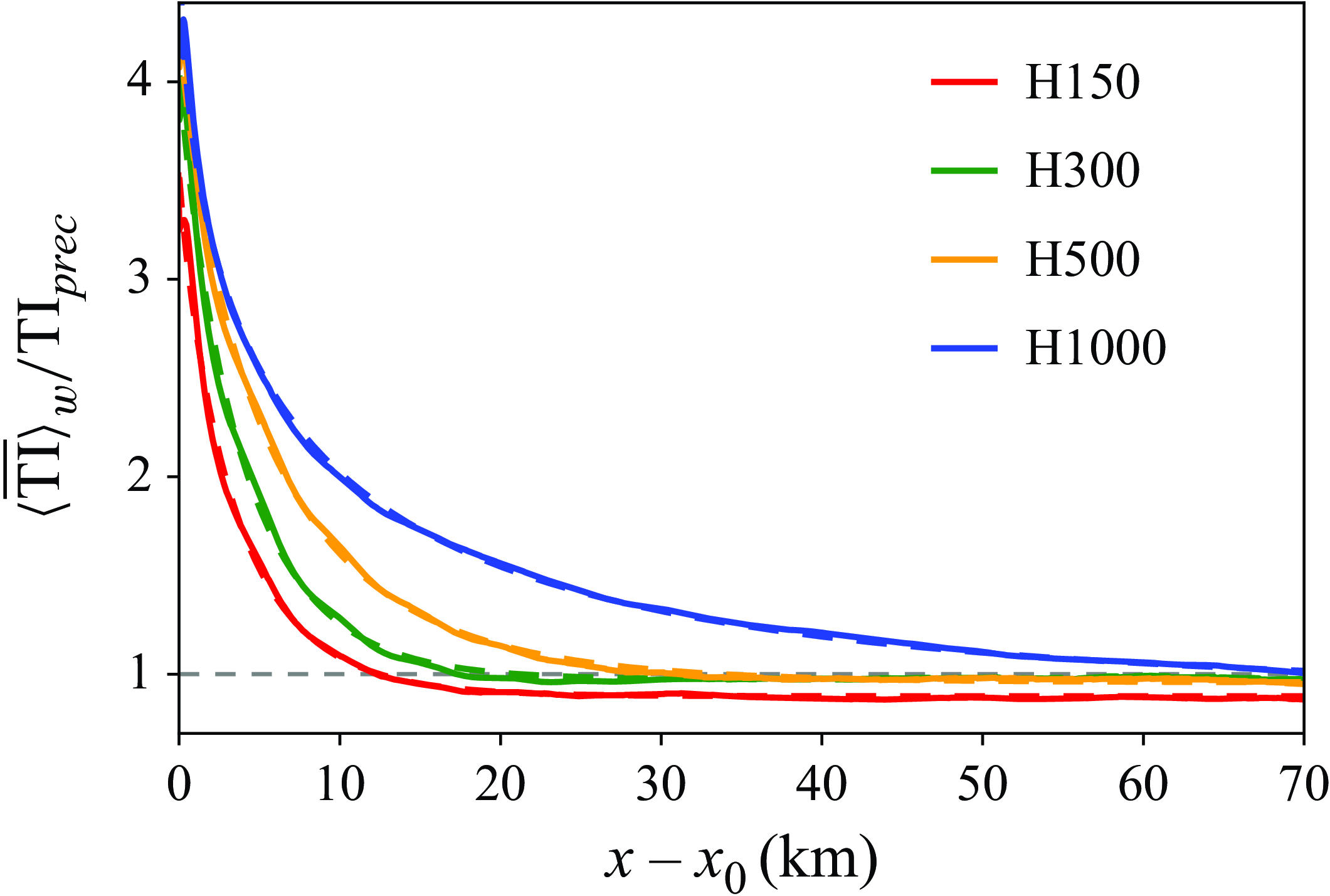
To conclude, we show in figure 16 the turbulence intensity measured at hub height and as a function of the streamwise direction. We note that these profiles are further averaged along the
 $y$
direction over the wake width evaluated with the model reported in (4.1). For case H150, the turbulence intensity attains a constant value
 $20$
km downwind of the farm, while
 $50$
km is necessary in case H1000 for the farm-added turbulence intensity to decay. While the turbulence intensity tends to the precursor value in cases H500 and H1000, a lower value is attained in shallow-boundary-layer cases due to the reduced wind shear within the turbine rotor disk with respect to the background flow. Similarly to Maas (Reference Maas2023a
), we observe that the decay of the turbulence intensity can be well approximated by the expression
 $a_{t} \exp(-b_{t} (x-x_0)^{c_t} ) +d_{t}$
, where
 $\Phi _{{TI}} = [a_{t} ,b_{t} ,c_{t} ,d_{t}]$
represents a set of fitting parameters, and
 $x_0=30$
km denotes the beginning of the wake region. The dashed lines in figure 16 represent the fitting function. The fitting parameters for each capping-inversion height are reported in the caption of figure 16. These parameters can support the development and calibration of turbulence intensity parametrisations for engineering wake models (Crespo & Hernandez Reference Crespo and Hernandez1996).
Time-averaged turbulence intensity further averaged over the wake width as a function of the streamwise direction further normalised with the turbulent intensity value attained in precursor simulation – see table 1. The dashed lines are obtained using the expression
 $a_t \exp(-b_t(x-x_0)^{c_t}) +d_t$
, with
 $x_0=30$
km, and
 $\Phi _{\textit{TI}} = [a_t,b_t,c_t,d_t]$
is the set of fitting parameters, with
 $\Phi _{\textit{TI}}^{H150}=[8.79,0.34,0.88,2.94]$
,
 $\Phi _{\textit{TI}}^{H300}=[10.44,0.29,0.92,3.30]$
,
 $\Phi _{\textit{TI}}^{H500}=[12.72,0.25,0.81,3.61]$
and
 $\Phi _{\textit{TI}}^{H1000}=[16.21,0.39,0.52,3.59]$
. The
 $x$
-axis is rescaled with
 $x_0=30$
km, which denotes the beginning of the wake region.

4.3. Streamwise momentum budget analysis
To highlight the dominant recovery mechanisms for the different cases, we perform a streamwise momentum budget analysis. A mass balance analysis is also performed, with results reported in Appendix C. We remark that in both analyses, we focus solely on the region downwind of the farm. We refer to Lanzilao (Reference Lanzilao2023) and Lanzilao & Meyers (Reference Lanzilao and Meyers2024b ) for an in-depth analysis of the momentum and energy budget upstream and within the farm.
The momentum analysis adopts a control volume
 $\Omega$
that measures
 $s_x D/2$
along the streamwise direction. The vertical dimension of the control volume coincides with the turbine rotor height, i.e. from
 $z_1 = z_h - D/2$
to
 $z_2 = z_h + D/2$
. Since we focus on the momentum balance within the farm wake, the lateral extension of
 $\Omega$
is dictated by the wake width provided by the fitting model discussed in § 4.2. Hence the lateral faces of the control volume change location along the streamwise direction and are defined as
 $y_1 = y_r + \delta _r/2$
and
 $y_2=y_l-\delta _l/2$
(i.e. the centreline of the mixing layers). We note that we assume the lateral edges of the control volume to be constant with height, meaning that
 $y_1$
and
 $y_2$
are not functions of
 $z$
. Figure 13 shows that this is a valid assumption, apart from case H150 where the farm wake abruptly deviates clockwise at the turbine-tip height. In summary, a generic control volume
 $\Omega _i$
has dimensions
 $s_x D/2 \times \delta _{{wake}}(x_i) \times D$
. We remark that we denote with
 $x_1$
,
 $x_2$
,
 $y_1$
,
 $y_2$
,
 $z_1$
and
 $z_2$
the boundaries of the control volume, while the
 $y$
–
 $z$
,
 $x$
–
 $z$
and
 $x$
–
 $y$
faces are denoted with
 $\Gamma _x$
,
 $\Gamma _y$
and
 $\Gamma _z$
.
Streamwise variation of momentum sources and sinks for case H300 normalised by the time-averaged total wind-farm thrust force and the control volume width: (a) all terms of (4.2), including
 $\mathcal{S}=\Delta \mathcal{A}_{uu,x} + \Delta \mathcal{A}_{uw,z} + \mathcal{P}_x$
; (b) the contribution of each added in the
 $\mathcal{S}$
term. Only the region downwind of the farm is considered, so the term
 $\mathcal{F}_{t,x}$
has no contribution. The
 $x$
-axis is rescaled with
 $x_0=30$
km, which denotes the beginning of the wake region.

The budget equation is obtained by taking a time average of the streamwise momentum equation, further integrating it over the control volume
 $\Omega$
to average out local oscillations. Additionally, we apply the divergence theorem, enabling us to eliminate the divergence operator and transition from a volume to a surface integral. As a result, the streamwise momentum equation for any control volume
 $\Omega$
reads as
 \begin{equation} \begin{aligned} &\underbrace {-\Big [ \int _{\Gamma _x} \bar {u}\bar {u}\, {\rm d}\Gamma _x\Big ]_{x_1}^{x_2}}_{\Delta \mathcal{A}_{uu,x}} \underbrace {-\Big [ \int _{\Gamma _y} \bar {u}\bar {v}\, {\rm d}\Gamma _y\Big ]_{y_1}^{y_2}}_{\Delta \mathcal{A}_{uv,y}} \underbrace {-\Big [ \int _{\Gamma _z} \bar {u}\bar {w}\, {\rm d}\Gamma _z\Big ]_{z_1}^{z_2}}_{\Delta \mathcal{A}_{uw,z}} \underbrace{{-}\Big [ \int _{\Gamma _x} \Big (\overline {u'u'}^r+\overline {u'u'}^{{sgs}} \Big )\, {\rm d} \Gamma _x \Big ]_{x_1}^{x_2}}_{\Delta \mathcal{F}_{uu,x}}\\[5pt] & \underbrace {-\Big [ \int _{\Gamma _y} \Big (\overline {u'v'}^r+\overline {u'v'}^{{sgs}} \Big )\, {\rm d} \Gamma _y \Big ]_{y_1}^{y_2}}_{\Delta \mathcal{F}_{uv,y}} \underbrace {-\Big [ \int _{\Gamma _z} \Big (\overline {u'w'}^r+\overline {u'w'}^{{sgs}} \Big )\, {\rm d} \Gamma _z \Big ]_{z_1}^{z_2}}_{\Delta \mathcal{F}_{uw,z}} \\[5pt] &{}+\underbrace {\int _\Omega f_c \overline {v}\, {\rm d}\Omega }_{\mathcal{C}_x} \underbrace {{}-\int _\Omega \frac {1}{\rho _o} \frac {\partial \overline {p}^\ast }{\partial x}\, {\rm d}\Omega }_{\mathcal{P}_x} \underbrace {{}-\int _\Omega \frac {1}{\rho _o} \frac {\partial \overline {p}_{\infty }}{\partial x}\, {\rm d}\Omega }_{\mathcal{P}_{\infty ,x}} + \underbrace {\int _\Omega \overline {f}_x\, {\rm d}\Omega }_{\mathcal{F}_{t,x}}= 0, \end{aligned} \end{equation}
where
 $u'=u-\bar {u}$
. The terms
 $\Delta \mathcal{A}_{uu,x}$
,
 $\Delta \mathcal{A}_{uv,y}$
and
 $\Delta \mathcal{A}_{uw,z}$
represent the advection of streamwise momentum by the streamwise, spanwise and vertical velocity. The terms
 $\Delta \mathcal{F}_{uu,x}$
,
 $\Delta \mathcal{F}_{uv,y}$
and
 $\Delta \mathcal{F}_{uw,x}$
denote the total (i.e. resolved + modelled) turbulent transport of streamwise momentum along the streamwise, spanwise and vertical directions. Further,
 $\mathcal{C}_x$
denotes the contribution of the Coriolis force,
 $\mathcal{P}_x$
and
 $\mathcal{P}_{\infty ,x}$
represent the contributions of the streamwise pressure gradients induced by the wind-farm forcing and the background pressure gradient, and
 $\mathcal{F}_{t,x}$
indicates the turbine forcing term. The latter term is zero out of the wind-farm region and therefore is not included in the analysis below. We note that due to the sign convention chosen, the first six terms in (4.2) are positive when the mean flow or turbulence transports more momentum in than out of the control volume, and negative when the opposite occurs. For example, the term
 $\Delta \mathcal{A}_{uu,x}$
is positive when
 $\bar {u} \bar {u}$
integrated over
 $\Gamma _{x_1}$
is higher than when integrated over
 $\Gamma _{x_2}$
, meaning that an increase in streamwise velocity along the
 $x$
direction causes this term to be negative.
Streamwise variation of momentum sources and sinks for case H1000 normalised by the time-averaged total wind-farm thrust force and the control volume width: (a) all terms of (4.2), including
 $\mathcal{S}=\Delta \mathcal{A}_{uu,x} + \Delta \mathcal{A}_{uw,z} + \mathcal{P}_x$
; (b) the contribution of each added in the
 $\mathcal{S}$
term. We note that only the region downwind of the farm is considered, so the term
 $\mathcal{F}_{t,x}$
has no contribution. The
 $x$
-axis is rescaled with
 $x_0=30$
km, which denotes the beginning of the wake region.

Figure 17(a) shows the streamwise evolution of all terms of (4.2) for case H300. The close vicinity of the capping inversion to turbine-tip height dampens the vertical turbulent entrainment of momentum. In fact,
 $\Delta \mathcal{F}_{uw,z}$
drops abruptly in the first
 $5$
km, attaining a similar value to that observed in the precursor simulation. This term contributes to the replenishment of the wake only in the near-wake region, where a fast recovery rate is observed – see e.g. Figure 12(c). Further,
 $\Delta \mathcal{F}_{uu,x}$
also attains a positive value in the near-wake region. However, this term is about three times smaller than
 $\Delta \mathcal{F}_{uw,z}$
, and it becomes negligible
 $5$
km downstream of the farm. The spanwise advection of mean flow
 $\Delta \mathcal{A}_{uv,y}$
is negligible in the first
 $10$
km of the wake, but becomes the dominant term contributing to the wake recovery in the far-wake region. However, flow advection along the spanwise direction is far less efficient than the vertical transfer of momentum in the wake recovery process. As a consequence, the velocity deficit shows a very slow recovery rate. Similarly to Bastankhah et al. (Reference Bastankhah, Mohammadi, Lees, Diaz, Buxton and Ivanell2024), we note a negligible contribution of the Coriolis term
 $\mathcal{C}_x$
, together with the spanwise turbulent transport of momentum. The background pressure gradient term
 $\mathcal{P}_\infty$
brings a positive contribution, although it speeds up the flow throughout the whole domain. Finally, we group terms that show an oscillatory behaviour into
 $\mathcal{S}=\Delta \mathcal{A}_{uu,x} + \Delta \mathcal{A}_{uw,z} + \mathcal{P}_x$
, which is the sum of mean advection along the streamwise and vertical directions and pressure perturbation. The contribution of each term is shown in figure 17(b). The strong oscillatory behaviour is due to the presence of trapped waves, which considerably alter the flow behaviour within the ABL when
 $H$
is low. In fact, the gravity-wave horizontal wavelength predicted using linear theory measures approximately
 $4.5$
km (see Vosper Reference Vosper2004; Sachsperger, Serafin & Grubišić Reference Sachsperger, Serafin and Grubišić2015), which is in line with the period of the oscillations shown in figure 17(b). We note that this mechanism in not visible in the results of Bastankhah et al. (Reference Bastankhah, Mohammadi, Lees, Diaz, Buxton and Ivanell2024) as they fixed the capping-inversion height. Here, we can also observe that
 $\Delta \mathcal{A}_{uu,x}$
is out of phase with respect to
 $\Delta \mathcal{A}_{uw,z}$
, while the latter is in phase with
 $\mathcal{P}_x$
. This behaviour can be explained through continuity. In fact, as the flow accelerates (
 $\Delta \mathcal{A}_{uu,x}$
negative), it also moves downwards (
 $\Delta \mathcal{A}_{uw,z}$
positive), and vice versa. Moreover, a positive
 $\mathcal{P}_x$
value corresponds to a favourable pressure gradient, which causes the flow to locally accelerate, therefore generating this out-of-phase behaviour with
 $\Delta \mathcal{A}_{uu,x}$
. The fact that both
 $\Delta \mathcal{A}_{uu,x}$
and
 $\Delta \mathcal{A}_{uw,z}$
do not attain a zero value in the far-wake region underlines that the wake does not fully recover.
(a) Streamwise variation of
 $\Delta \mathcal{F}_{uw,z}$
(solid line) and
 $\Delta \mathcal{A}_{uv,y}$
(dashed line) normalised by the time-averaged total wind-farm thrust force of the respective cases and the control volume width. (b) Sum of the advection terms
 $\mathcal{A} = \Delta \mathcal{A}_{uu,x} + \Delta \mathcal{A}_{uv,y} + \Delta \mathcal{A}_{uw,z}$
normalised by the time-averaged total wind-farm thrust force of the respective cases and the control volume width. The
 $x$
-axis is rescaled with
 $x_0=30$
km, which denotes the beginning of the wake region.

The same analysis for case H1000 is shown in figure 18. The main difference from case H300 is the strong vertical turbulent entrainment of momentum in the first
 $20$
km of the wake, which causes the velocity deficit to rapidly recover. Since the wake is partially recovered after
 $20$
km, the advection of spanwise momentum by the streamwise velocity remains negligible. Similarly to case H300,
 $\Delta \mathcal{F}_{uu,x}$
,
 $\Delta \mathcal{F}_{uv,y}$
and
 $\mathcal{C}_x$
have negligible contributions. Figure 18(b) illustrates the components of the
 $\mathcal{S}$
term. Here, we can observe that the flow is accelerating and moving downwards (i.e. negative
 $\Delta \mathcal{A}_{uu,x}$
and positive
 $\Delta \mathcal{A}_{uw,z}$
). Similarly to Bastankhah et al. (Reference Bastankhah, Mohammadi, Lees, Diaz, Buxton and Ivanell2024), we note that the strong flow acceleration is attained approximately where the vertical turbulent transport of momentum is also high, resulting in a strong correlation between the terms
 $\Delta \mathcal{A}_{uu,x}$
and
 $\Delta \mathcal{F}_{uw,z}$
. Moreover, although
 $\Delta \mathcal{A}_{uw,z}$
oscillates along the streamwise direction, its magnitude is on average slightly higher than
 $\Delta \mathcal{F}_{uw,z}$
, meaning that the vertical advection of mean flow plays an important role in the wake recovery process. We note that the H1000 case has the same oscillatory frequency as case H300. This is due to the fact that the horizontal trapped-wave wavelength depends on the capping-inversion strength and free-atmosphere lapse rate, which are equal for the two cases. We also observe the same in-phase and out-of-phase behaviour, although the magnitude of the oscillations caused by interfacial gravity waves is smaller than case H300 due to the higher distance between the turbine region and the capping-inversion height. Moreover, both
 $\Delta \mathcal{A}_{uu,x}$
and
 $\Delta \mathcal{A}_{uw,z}$
tend to zero at the end of the wake region, denoting that the wake has mostly recovered.
Excluding the terms heavily influenced by oscillation due to the presence of gravity waves, the two dominant terms that contribute to wake recovery are
 $\Delta \mathcal{F}_{uw,z}$
and
 $\Delta \mathcal{A}_{uv,y}$
, which are shown for all cases in figure 19(a). We can see that the vertical turbulent entrainment of momentum is directly proportional to
 $H$
. In fact, in deep-boundary-layer cases, the wake is mostly recovered within the first
 $20$
–
 $30$
km downwind of the farm, leaving a negligible role to the flow advection in the spanwise direction. Contrarily,
 $\Delta \mathcal{F}_{uw,z}$
dies out abruptly in shallow boundary layers, therefore causing very long wind-farm wakes, which are slowly replenished by the advection of spanwise momentum by the streamwise velocity. Interestingly, we note that the
 $\Delta \mathcal{F}_{uw,z}$
and
 $\Delta \mathcal{A}_{uv,y}$
profiles intersect in proximity of the zero line, except for case H150. Next, figure 19(b) shows
 $\mathcal{A} = \Delta \mathcal{A}_{uu,x} + \Delta \mathcal{A}_{uv,y} + \Delta \mathcal{A}_{uw,z}$
, i.e. the sum of the advection terms. We can observe oscillations that gradually decrease in amplitude along the streamwise direction, which denote a net acceleration and deceleration of the flow induced by trapped waves. In the far wake,
 $\mathcal{A}$
tends to a negative value for shallow-boundary-layer cases, denoting that the wake is still accelerating. This is in accordance with the results shown in figure 12(c). However, in deep-boundary-layer cases,
 $\mathcal{A}$
tends to small negative values in the far wake. In fact, the wake is mostly recovered by the vertical turbulent entrainment within the first 20–30 km downwind of the farm, leaving a negligible role to the flow advection. We remark that all cases share the same potential temperature profile above the ABL, resulting in in-phase profiles of
 $\mathcal{A}$
up to approximately 40 km downstream of the farm.
Time-averaged advection of (a,b) spanwise momentum by the streamwise velocity and (c,d) total spanwise turbulent transport of momentum, as functions of the spanwise direction obtained at
 $x=x_0$
(brightest yellow) and
 $x=x_0+70$
(darkest blue), with increments of
 $5$
km in between, for cases (a,c) H300 and (b,d) H1000. Each symbol denotes a spanwise average over one turbine spacing (i.e.
 $5D$
), while the vertical yellow and blue lines denote the location of the wake edges at
 $x=x_0$
and
 $x=x_0+70$
, respectively, where
 $x_0=30$
km indicates the beginning of the wake region.

To further investigate the spanwise advection of mean flow and spanwise turbulent transport of momentum, we analyse the quantities
 $\bar {u} \bar {v}$
and
 $\overline {u' v'}$
along the
 $y$
direction at hub height, taken at locations downwind of the farm (i.e. from
 $x=x_0$
to
 $x=x_0+70$
with increments of
 $5$
km). figure 20(a,b) display the spanwise advection of mean flow for cases H300 and H1000, respectively. In the shallow-boundary-layer case, we observe a high value of
 $\bar {u} \bar {v}$
at the location of the wake right edge (i.e.
 $y\approx 45$
km), which further increases along the downstream direction. Within the wake region, we observe a constant and positive spanwise advection that decreases significantly in proximity to the left edge of the wake (i.e.
 $y\approx 55$
km). In the H1000 case, the spanwise advection of mean flow attains a very similar magnitude at the wake edges, resulting in low
 $\Delta \mathcal{A}_{uv,y}$
values. In the far-wake region, we observe a higher spanwise advection of mean flow on the left edge. However, the wake deficit is almost fully recovered at these streamwise locations. Next, figure 20(c,d) illustrate the spanwise turbulent transport of momentum for cases H300 and H1000. In the shallow-boundary-layer case, this term is close to zero within the wake, attaining higher values in proximity of the left edge of the wake, where a steep spanwise gradient of streamwise velocity takes place – see figure 11(b). Since the latter increases in magnitude along the streamwise direction, we observe the peak in
 $\overline {u' v'}$
increasing as well. A similar behaviour is observed in the H1000 case, although higher fluctuations of
 $\overline {u' v'}$
are attained within the wake region. However, the role of the spanwise turbulent transport of momentum in the wake recovery process remains negligible since this term is approximately two orders of magnitude smaller than
 $\bar {u} \bar {v}$
.
4.4. Spanwise momentum budget analysis
In this analysis we adopt the same control volumes
 $\Omega$
used in § 4.3, but we investigate the budget terms for the spanwise momentum equation. The latter reads as
 \begin{equation} \begin{aligned} &\underbrace {-\bigg [ \int _{\Gamma _x} \bar {u}\bar {v}\, {\rm d}\Gamma _x\bigg ]_{x_1}^{x_2}}_{\Delta \mathcal{A}_{uv,x}} \underbrace {{}-\bigg [ \int _{\Gamma _y} \bar {v}\bar {v}\, {\rm d}\Gamma _y\bigg ]_{y_1}^{y_2}}_{\Delta \mathcal{A}_{vv,y}} \underbrace {{}-\bigg [ \int _{\Gamma _z} \bar {v}\bar {w}\, {\rm d}\Gamma _z\bigg ]_{z_1}^{z_2}}_{\Delta \mathcal{A}_{vw,z}} \\[5pt] &\underbrace {{}-\bigg [ \int _{\Gamma _x} \bigl (\overline {u'v'}+\overline {\tau }_{12}^{{sgs}} \bigl )\, {\rm d} \Gamma _x \bigg ]_{x_1}^{x_2}}_{\Delta \mathcal{F}_{uv,x}} \underbrace {-\bigg [ \int _{\Gamma _y} \bigl (\overline {v'v'}+\overline {\tau }_{22}^{{sgs}} \bigl )\, {\rm d} \Gamma _y \bigg ]_{y_1}^{y_2}}_{\Delta \mathcal{F}_{vv,y}} \underbrace {-\bigg [ \int _{\Gamma _z} \bigl (\overline {v'w'}+\overline {\tau }_{23}^{{sgs}} \bigl )\, {\rm d} \Gamma _z \bigg ]_{z_1}^{z_2}}_{\Delta \mathcal{F}_{vw,z}} \\[5pt] &\underbrace {{}-\int _\Omega f_c \overline {u}\, {\rm d}\Omega }_{\mathcal{C}_y} \underbrace {{}-\int _\Omega \frac {1}{\rho _o} \frac {\partial \overline {p}^\ast }{\partial y}\, {\rm d}\Omega }_{\mathcal{P}_y^\ast } \underbrace {{}-\int _\Omega \frac {1}{\rho _o} \frac {\partial \overline {p}_\infty }{\partial y} \,{\rm d}\Omega }_{\mathcal{P}_{\infty ,y}} \underbrace {{}+\int _\Omega \overline {f}_y\, {\rm d}\Omega }_{\mathcal{F}_{t,y}}= 0. \end{aligned} \end{equation}
The terms
 $\Delta \mathcal{A}_{uv,x}$
,
 $\Delta \mathcal{A}_{uv,y}$
and
 $\Delta \mathcal{A}_{vw,z}$
represent the advection of spanwise momentum by the streamwise, spanwise and vertical velocity. The terms
 $\Delta \mathcal{F}_{uv,x}$
,
 $\Delta \mathcal{F}_{vv,y}$
and
 $\Delta \mathcal{F}_{vw,z}$
denote the total (i.e. resolved + modelled) turbulent transport of spanwise momentum along the streamwise, spanwise and vertical directions. Further,
 $\mathcal{C}_y$
denotes the contribution of the Coriolis force,
 $\mathcal{P}_y$
and
 $\mathcal{P}_{\infty ,y}$
represent the contributions of the spanwise pressure gradients induced by the wind-farm forcing and the background pressure gradient, and
 $\mathcal{F}_{t,y}$
indicates the turbine forcing term. The latter term is zero out of the wind-farm region and therefore is not included in the analysis below. Moreover, we adopt the same sign convention as used in § 4.3.
Spanwise variation of momentum sources and sinks for cases (a) H150, (b) H300, (c) H500 and (d) H1000 normalised by the time-averaged total wind-farm thrust force and the control volume width. Only the region downwind of the farm is considered, so the term
 $\mathcal{F}_{t,y}$
has no contribution. The
 $x$
-axis is rescaled with
 $x_0=30$
km, which denotes the beginning of the wake region.

Figure 21 illustrates the spanwise momentum sources and sinks for all cases. The spanwise background pressure gradient is related to
 $f_c G \cos\alpha$
and is therefore constant along the streamwise direction. The contribution of the Coriolis force is proportional to the streamwise velocity, and it increases in magnitude along the streamwise direction as a results of the wake recovery. In the free atmosphere,
 $\mathcal{P}_{\infty ,y} + \mathcal{C}_y = 0$
. However, the momentum sink generated by the farm decreases the magnitude of the Coriolis force, so that
 $\mathcal{P}_{\infty ,y} + \mathcal{C}_y \gt 0$
in the turbine region. This imbalance is compensated by
 $\mathcal{P}_y$
in cases H150, H300 and H500, which assumes a negative value denoting the presence of an opposing pressure gradient along the spanwise direction, as also observed in figure 7(m–o). The magnitude of this opposing spanwise pressure gradient is inversely related to
 $H$
and may explain the lack of growth in the mixing layer located on the left side of the farm (i.e.
 $\delta _l$
), as shown in figure 12(d). The oscillatory behaviour in
 $\mathcal{P}_y$
is related to the presence of atmospheric gravity waves. In case H1000,
 $\mathcal{P}_y \approx 0$
and the imbalance between background pressure gradient and Coriolis force is compensated by the turbulent transport of spanwise momentum along the vertical direction. We note that the term
 $\Delta \mathcal{F}_{vw,z}$
is non-negligible also in case H500, but contributes only in the first 10 km downwind of the farm, while it becomes close to zero in shallow boundary layers due to the vicinity of the inversion layer to turbine-tip height. All other terms reported in figure 21 are negligible, assuming values of the order of the residual.
5. Conclusions
The aim of this work is to bring new physical insights into the wake behaviour of large-scale wind farms operating in CNBLs with various capping-inversion heights. To this end, we performed four simulations of a single wind farm using SP-Wind, an LES solver developed at KU Leuven. The main domain was driven by turbulent fully developed statistically steady flow fields obtained in precursor simulations. Moreover, the solver periodicity in the streamwise direction was broken using a wave-free fringe region technique, while at the top of the domain, an RDL was placed to damp gravity waves. A large numerical domain with length, width and height
 $110 \times 100 \times 25$
km
 $^3$
was used to allow the wake to fully develop and to minimise artificial effects due to the domain boundaries.
In shallow boundary layers, such as cases H150 and H300, the vicinity of the capping inversion to the turbine-tip height limits the wake development in the vertical direction. Moreover, the capping inversion behaves as a pliant surface, limiting flow entrainment from the free atmosphere. Consequently, these cases show strong velocity deficits in the farm wake, and a very slow recovery rate. The strong flow deceleration attained in these two cases decreases the Coriolis force magnitude. Therefore, the wake turns towards the direction of the background pressure gradient, which is an anticlockwise flow rotation in the northern hemisphere. In cases H500 and H1000, the increase in the
 $H/z_{{tip}}$
ratio allows the formation of a high-speed channel between the tip height and the capping-inversion base that enhances vertical turbulent entrainment of momentum into the wake, therefore giving rise to a lower velocity deficit and a faster recovery rate. The vertical entrainment of momentum adds clockwise-turning flow from aloft into the wake region. Therefore, a clockwise wake deflection is observed, which is dictated by the wind veer present in the background flow. This also means that in flows with small wind veer, the wind-farm wake would turn anticlockwise. Despite a distance of approximately
 $75$
km from the last-row turbine to the fringe region, in none of the cases was the wake fully replenished, with velocity deficits with respect to the inflow up to
 $25$
% measured
 $70$
km downstream of the farm in shallow boundary layers. Similar to previous studies, we observed a much faster recovery in terms of TKE, which drops below the background value within the first
 $10$
–
 $20$
km into the wake.
Defining a wake region together with estimating wake properties is non-trivial. Therefore, we proposed a simple fitting model for the spanwise velocity magnitude profiles at streamwise locations downwind of the farm. The latter allowed us to evaluate wake properties such as the wake strength, width and deflection together with identifying the presence of two distinct mixing layers at both sides of the wake in cases where
 $\delta _{{wake}}/H \gg 1$
, and track their streamwise evolution. We observed that the centreline of the mixing layers turned towards the low-velocity region, therefore resulting in a decreasing wake width along the streamwise direction for all cases, with a wake-to-farm width ratio going from approximately
 $1.2$
to
 $1$
over a distance of
 $70$
km. The wake centre predicted by the fitting model allowed us to clearly observe how the capping-inversion height influences the wake deflection, generating a clear distinction between shallow and deep boundary layers. Moreover, we observed a very fast recovery rate in the first
 $5$
km into the wake, which slows down considerably further downwind. Furthermore, the model allowed us to observe that the wake edges and centre do not vary across the rotor height, except for case H150, where a significant clockwise rotation at tip height takes place. This effect is caused by the strong wind veer attained within the capping inversion, which is very near to tip height in this case. We remark that this model has the only function of identifying the wake location and shape, and is not subjected to constraints for the conservation of mass and momentum. Finally, we investigated the wake development along the vertical direction, noticing that the wake spreads up to the capping-inversion height, which significantly limits the wake growth in shallow-boundary-layer cases.
To highlight the dominant wake recovery mechanisms, we performed a streamwise and spanwise momentum budget analysis. We found that the two dominant terms that contribute to wake recovery are the vertical turbulent entrainment of momentum and the advection of streamwise momentum by the spanwise velocity. However, their contributions differ depending on the capping-inversion height. In shallow boundary layers, the close vicinity of the capping inversion to turbine-tip height dampens the vertical turbulent entrainment of momentum, which drops abruptly in the first
 $5$
km into the wake. Consequently, the wake is mostly recovered by spanwise mean flow entrainment, which is rather inefficient, therefore causing very long wakes with strong deficits. Further, we noticed that the spanwise entrainment of mean momentum occurs mostly on the right edge of the wake. In fact, an anticlockwise flow motion near the left edge of the wake, which persists at each location downstream of the farm, provokes strong local spanwise gradients of streamwise velocity, and significantly limits the spanwise entrainment of mean flow in this region. In deep boundary layers, the wake is mostly recovered by vertical turbulent entrainment of momentum, and spanwise entrainment has a negligible contribution. In such cases, the wind veer profiles in the wake region and at its sides are very similar, and the effects of trapped waves on the flow behaviour are limited. Consequently, we do not observe regions of flow recirculation and convergence at the wake edges.
Finally, we conducted a study on the sensitivity of the numerical solution to the grid resolution and domain width, using the H300 precursor flow fields to drive the simulations. Interestingly, we found that the error caused by coarsening the grid resolution is an order of magnitude smaller than the error introduced by using a domain with a too low
 $L_y/L_y^f$
ratio. Moreover, we observed that doubling the grid cell size in the streamwise and spanwise directions does not alter the wake properties. However, a domain with ratio
 $L_y/L_y^f=3.19$
displays a narrower farm wake with a faster recovery rate than the one observed in a domain with
 $L_y/L_y^f=9.57$
. Therefore, particularly when simulating shallow boundary layers, we recommend using a sufficiently wide domain at the expense of using a coarser numerical grid.
In the current work, we focused solely on the wake development of a single farm. However, farms are typically clustered together nowadays. Therefore, a natural extension of this work consists in considering the wake behaviour of a cluster of farms. This would also allow us to better investigate farm–farm interactions, together with their effects on power losses and loads, as well as assessing the potential of wind-farm wake mitigation techniques, such as yaw control. Furthermore, the study assumes the presence of statistically steady state conditions, which rarely occur in a real scenario. Therefore, we are planning to drive our simulations using mesoscale forcing to also account for the effects of the natural variability in the inflow conditions on the wake development. This would also allow us to compare our findings against wind-farm wake profiles observed in SAR images. This study limited its scope to CNBLs with different capping-inversion heights. However, we are aware that the wake dynamic is also affected by other parameters, such as the capping-inversion strength, the free-atmosphere lapse rate, the surface roughness, the geostrophic wind, the Coriolis force and the farm geometry, among others. Therefore, future research should focus on investigating farm wake strength and deflection over a wider set of parameters, also including stable and convective boundary layers. Finally, analytical wake models are known to over-predict the wake recovery rate. Therefore, the set of simulations analysed in this work can be used as a benchmark for future development and calibration of faster engineering models.
Acknowledgements.
The authors thank S. Vandenbrande for HPC technical support.
Funding.
The authors acknowledge support from the Research Foundation Flanders (FWO, grant no. G0B1518N), from the project FREEWIND, funded by the Energy Transition Fund of the Belgian Federal Public Service for Economy, SMEs, and Energy (FOD Economie, K.M.O., Middenstand en Energie), and from the European Union Horizon Europe Framework programme (HORIZON-CL5-2021-D3-03-04) under grant agreement no. 101084205. The computational resources and services in this work were provided by the VSC (Flemish Supercomputer Centre), funded by the Research Foundation Flanders (FWO) and the Flemish Government department EWI.
Declaration of interests.
The authors report no conflict of interest.
Data availability statement.
The full dataset underlying the analysis in the current paper, including e.g, turbine statistics, and three-dimensional time-averaged flow fields of first- and second-order statistics of precursor and main domains, as well as some post-processing example scripts, is available open source as a KU Leuven RDR dataset: https://doi.org/10.48804/LRSENQ (Lanzilao & Meyers Reference Lanzilao and Meyers2024a ).
Author contributions.
L.L. and J.M. jointly set up the simulation studies and wrote the manuscript. L.L. performed code implementations and carried out the simulations. J.M. supervised the research and was responsible for acquisition of funding.
Appendix A. Influence of the horizontal grid resolution and domain width on the numerical results
The simulations presented in this paper were initially performed on a domain with width
 $30$
km and a finer horizontal grid resolution. However, Lanzilao & Meyers (Reference Lanzilao and Meyers2024b
) have shown that the domain width can have major influences on the results in simulations of wind farms operating in CNBLs. In particular, they recommended a
 $L_y/L_y^{f}$
ratio of at least 6 in the presence of shallow boundary layers. Therefore, we have re-run all cases on a wider domain. Moreover, we have used a coarser grid resolution, to keep the computational cost manageable. This new set of simulations is the one analysed in the main body of the paper. Here, we use the original batch of simulations to illustrate the influence of the domain width and grid resolution on the wake behaviour. We note that the comparison is made only with cases driven by the H300 precursor flow fields. For other set-up parameters, we refer the reader to § 2.
Two different numerical grids are analysed. Lanzilao & Meyers (Reference Lanzilao and Meyers2022a
, Reference Lanzilao and Meyers2023, Reference Lanzilao and Meyers2024b
) have used a horizontal grid with cell sizes
 $\Delta x/2$
and
 $\Delta y/2$
, where
 $\Delta x$
and
 $\Delta y$
measure 62.5 m and 43.48 m, respectively. We define this as the fine grid, which we use to run a simulation on a numerical domain with length and width
 $90$
km and
 $30$
km, respectively. This simulation will be denoted as the Ly-30-fine case. The second grid, which we define as coarse, uses a streamwise and spanwise grid size corresponding to
 $\Delta x$
and
 $\Delta y$
. Using this grid, we perform three additional simulations where the domain length is fixed to
 $90$
km while the width assumes values
 $30$
,
 $60$
and
 $90$
km. The latter cases will be denoted as Ly-30-coarse, Ly-60-coarse and Ly-90-coarse, respectively. Here, it is necessary to use a coarser grid to make the simulations affordable, given the very high number of DOF. The vertical grid and domain dimension correspond to those described in § 2.2, and are the same for all cases. The error caused by the coarsening of the horizontal grid can be estimated by comparing the Ly-30-fine and Ly-30-coarse cases, as the only differences here are streamwise and spanwise dimensions of the grid cell. The differences caused by the domain width can be estimated by comparing case Ly-30-coarse versus cases Ly-60-coarse and Ly-90-coarse, since the grid resolution is the same for all cases. The outcome of this analysis will allow us to choose a domain size and a numerical grid suitable for these types of simulations. We note that the cases considered in this Appendix are listed in table 2, where additional information about the cases set-up is reported.
Overview of the numerical domains used to perform the sensitivity study on the horizontal grid resolution and domain width. The parameters
 $L_x$
,
 $L_y$
and
 $L_z$
denote the streamwise, spanwise and vertical domain dimensions, while
 $N_x$
,
 $N_y$
and
 $N_z$
denote the numbers of grid points used along the respective directions. Here,
 $L_{{wake}}$
denotes the fetch of the domain between the last-row turbine location and the start of the fringe region, while
 $L_x^f$
and
 $L_y^f$
represent the wind-farm length and width, respectively. The last column reports the number of DOF comprehensive of both precursor and main domains. Each case is driven by the H300 precursor flow fields. The last row reports the selected domain used to perform the sensitivity study to the atmospheric state.

We start by discussing the impact of the horizontal grid resolution on the numerical simulation. First, we remark that the results in the precursor domain are not affected by the change in grid resolution. This is visible in figure 4. Therefore, all differences observed here are due solely to the flow dynamics in the main domain. figure 22(a,b) show the relative error in terms of velocity magnitude and the difference in terms of flow angle between cases Ly-30-fine and Ly-30-coarse. We observe that the velocity within the farm area at hub height is on average approximately 3–5 % higher when using the fine grid. The wake recovery appears to be slightly slower when using the coarse grid, although differences tend to zero towards the end of the domain. Overall, we observe that the major discrepancies are attained within the farm and on the left edge of the wake. This is expected since those are regions of strong velocity gradients. In terms of flow angle, we observe differences up to
 $1^\circ$
, which mostly occur in the far-wake region.
(a–c) Relative error in terms of velocity magnitude and (d–f) flow angle in an
 $x$
–
 $y$
plane taken at hub height. Plots (a,d) highlight differences due to the grid resolution, while (b,c,e,f) show differences due to the domain width. The location of the wind farm is indicated by the black rectangle.

Next, we discuss the impact of the domain width on the results. figure 22(c,d) show the comparison in terms of velocity magnitude and flow angle between cases Ly-30-coarse and Ly-60-coarse, where the ratio
 $L_y/L_y^f$
varies from 3.19 to 6.38. It is easy to observe how the impact of the domain width on the numerical results is at least one order of magnitude higher than that caused by the grid resolution. For instance, similarly to Lanzilao & Meyers (Reference Lanzilao and Meyers2024b
), we observe that a smaller domain over-estimates flow blockage, with the velocity being of the order of 10 % lower in front of the farm. Moreover, a narrower domain enhances the wake recovery rate and its anticlockwise deflection. The same phenomena are observed in figure 22(e,f), where we compare the Ly-30-coarse and Ly-90-coarse cases. Here, velocity differences in the far wake region reach values above 25 %, while differences in flow angle are up to
 $5^\circ$
.
(a,b) Wake width, wake centre and (c,d) right- and left mixing layer widths normalised with the farm width. (e,f) Velocity deficit with respect to
 $M_{{side}}$
and velocity magnitude at the sides of the wake normalised with the velocity magnitude obtained in the precursor domain at hub height. All quantities are predicted by the fitting model shown in (4.1). The
 $x$
-axis is rescaled with
 $x_0=30$
km, which denotes the beginning of the wake region.

We now discuss the differences in wake width, strength and deflection within the wake and at its sides by using the fitting model reported in (4.1). The results are shown in figure 23. By comparing cases Ly-30-fine and Ly-30-coarse, we can observe how the wake width and centre assume very similar values. A similar conclusion can be drawn when comparing the mixing layers width as well as the wake velocity deficit and
 $M_{{side}}$
. Therefore, we can conclude that doubling the grid cell size in the streamwise and spanwise directions has little influence on the wake properties. In terms of domain width, differences are noticeable, particularly when comparing cases Ly-30-coarse and Ly-90-coarse. Figure 23(a) shows that the wake narrows in both cases. However,
 $\delta _{{wake}}/L_y^f$
is approximately 0.05 larger in the Ly-90-coarse case. Further, figure 23(b) shows that a narrow domain artificially enhances the anticlockwise deflection of the wake. Figure 23(e) illustrates that the velocity deficit in the wake, here defined with respect to the precursor velocity at hub height, recovers faster in a narrower domain. The high-speed channels that develop at the sides of the wake in domains with low
 $L_y/L_y^f$
ratios can be responsible for this effect. Figure 23(f) shows a clear difference in the
 $M_{{side}}$
profile between cases Ly-30-coarse and Ly-90-coarse. In fact, the velocity at the sides of the wake keeps increasing along the streamwise direction in a narrow domain, reaching
 $M_{{side}}/M_{{prec}}$
values up to 1.1. This phenomenon was also observed by Lanzilao & Meyers (Reference Lanzilao and Meyers2024b
). In wide domains,
 $M_{{side}}$
reaches a peak
 $10$
km downstream of the farm, remaining constant afterwards.
The strength of the wake generated by a farm is dependent on the amount of force that the turbines exert on the flow. Therefore, we conclude this analysis by investigating how the total thrust
 $T$
that the farm exerts on the incoming flow depends upon the grid size and domain size. The results are reported in figure 24, which shows the relative error in terms of thrust force. Doubling the size of the horizontal grid cells in the
 $x$
and
 $y$
directions introduces relative error
 $2\,\%$
on
 $T$
. However, tripling the domain width induces a difference of approximately
 $7\,\%$
.
We note that the presence of periodic boundary conditions in the horizontal directions allows for alternative interpretations of these results. For instance, when the domain width is
 $30$
km and the
 $L_y/L_y^f$
ratio measures 3.19, this would correspond to an infinite row of wind farms with spacing
 $L_y-L_y^f=20.6$
km. From this perspective, we can assert that the wake recovery rate in a row of wind farms is faster than that of an isolated farm, accompanied by a more pronounced wake deflection. Moreover, similarly to a single row of turbines (McTavish et al. Reference McTavish, Rodrigue, Feszty and Nitzsche2015), smaller spanwise distances between farms generate high-speed channels that can enhance the power output of a downstream farm. Although the simulations performed by Maas & Raasch (Reference Maas and Raasch2022) show similar results, the wake behaviour in clusters of farms requires more attention and further investigation.
In conclusion, we have observed that the wake behaviour is mostly insensitive to the grid resolutions adopted here. Moreover, the results indicate that a narrow domain alters substantially the wake properties, enhancing the wake recovery and altering the wake deflection. Moreover, domain length
 $90$
km with
 $L_{{wake}}/L_x^f=3.68$
does not suffice for attaining a full wake recovery (i.e. the wake is longer than
 $55$
km). As a result of this study, we fix the main domain length and width to
 $110$
km and
 $100$
km, respectively. This allows us to increase
 $L_{{wake}}/L_x^f$
to
 $5.68$
, while
 $L_y/L_y^f=10.64$
, which is well above the value 6 suggested by Lanzilao & Meyers (Reference Lanzilao and Meyers2024b
). Since results are quasi-independent of the grid size, we adopt the coarse grid, which implies
 $\Delta x=62.5$
m and
 $\Delta y=43.48$
m, with a total of
 $8.66 \times 10^9$
DOF. The selected numerical set-up is reported in table 2.
Relative error in terms of total farm thrust force for cases with different grid resolutions and domain widths.

Appendix B. Influence of the capping-inversion thickness on the wake behaviour
The aim of this appendix is to investigate the sensitivity of the wake behaviour to the capping-inversion thickness. To this end, we will compare the results obtained in cases H300 and H500, which adopt capping-inversion thickness
 $100$
m, against case H300–
 $\Delta$
H500, which is a simulation performed using the same set-up as case H300 but with
 $\Delta H=500$
m. The time-averaged profiles over the last
 $4$
h of precursor simulation are displayed in figure 25. Here, we observe that a thicker capping inversion allows for a bigger growth of the ABL during the spin-up phase. In fact, the capping-inversion heights for cases H300 and H300–
 $\Delta$
H500 corresponds to
 $319$
m and
 $397$
m, respectively. Therefore, the differences in results between these two cases are due not only to a change in capping-inversion thickness, but also to a change in capping-inversion height.
Vertical profiles of (a) velocity magnitude, (b) total shear stress magnitude, (c) wind direction and (d) potential temperature averaged along the full horizontal directions and over the last
 $4$
h of the simulation. The grey dashed line denotes the turbine-hub height, while the black dashed lines are representative of the rotor dimensions. The results shown here refer only to the precursor simulations.

Figure 26(a,b) show side views of horizontal velocity magnitude averaged in the
 $y$
direction along the width of the farm for cases H300 and H300–
 $\Delta$
H500, respectively. Moreover, the black lines illustrate the base and top of the inversion layer computed by fitting the LES data with the Rampanelli & Zardi (Reference Rampanelli and Zardi2004) model, which clearly illustrates the difference in
 $\Delta H$
between the two cases. We can also observe a difference in velocity deficit, with a stronger wake attained in case H300. Despite the capping inversion being five times thicker in case H300–
 $\Delta$
H500, we observe that the velocity deficit does not penetrate into the inversion layer, which limits the vertical development of the wake.
Contours of the time-averaged horizontal velocity magnitude in an
 $x$
–
 $z$
plane further averaged along the farm width in the spanwise direction for cases (a) H300 and (b) H300–
 $\Delta$
H500. The black lines represent the bottom and top of the inversion layer computed with the Rampanelli & Zardi (Reference Rampanelli and Zardi2004) model. The locations of the turbine-rotor disks are indicated with vertical white lines.

(a,b) Wake width, wake centre and (c,d) right- and left mixing layer widths normalised with the farm width. (e,f) Velocity deficit with respect to
 $M_{{side}}$
, and velocity magnitude at the sides of the wake, normalised with the velocity magnitude obtained in the precursor domain at hub height. All quantities are predicted by the fitting model shown in (4.1). The
 $x$
-axis is rescaled with
 $x_0=30$
km, which denotes the beginning of the wake region.

Next, we discuss the differences in wake width, strength and deflection within the wake and at its sides by using the fitting model reported in (4.1). Since the capping-inversion height of case H300–
 $\Delta$
H500 is in between that of cases H300 and H500, we also include the latter case in these comparisons. Although the wake width at the beginning of the wake region is similar among the three cases, we can see in figure 27(a) that the wake narrowing is more accentuated in case H300–
 $\Delta$
H500. Further, figure 27(b) illustrates that case H300–
 $\Delta$
H500 has a very minor wake deflection. This means that the two opposite effects triggered by the Coriolis force that are responsible for a clockwise or anticlockwise flow rotation of the farm wake are in balance for this atmospheric state. figure 27(c,d) also show that the widths of the mixing layers located at the sides of the wake are comparable among the three cases. The velocity deficit with respect to
 $M_{{side}}$
is shown in figure 27(e). The recovery rate of case H300–
 $\Delta$
H500 is very similar to that of cases H300 and H500. However,
 $\Delta M$
is lower than case H300, as already observed in figure 26(b). Finally, the velocity at the wake sides is shown in figure 27(f). A thicker capping inversion reduces the flow-blockage effect, so that the flow acceleration at the wake sides is also reduced significantly. This explains the very similar trend observed for the
 $M_{{side}}$
profile of cases H300–
 $\Delta$
H500 and H500.
Finally, we compare the two dominant terms that contribute to wake recovery, i.e.
 $\Delta \mathcal{F}_{uw,z}$
and
 $\Delta \mathcal{A}_{uv,y}$
, between cases H300, H300–
 $\Delta$
H500 and H500. The results are shown in figure 28. The vertical turbulent entrainment of momentum in case H300–
 $\Delta$
H500 shows a slower decay than in case H300 along the streamwise direction. However, its magnitude is still lower than in case H500. The mean flow entrainment along the spanwise direction is twice as strong as in case H500, and even higher than in case H300, particularly in the far-wake region. The combination of these two factors makes the wake recovery rate in case H300–
 $\Delta$
H500 faster than in case H300, but still slower with respect to case H500.
Streamwise variation of
 $\Delta \mathcal{F}_{uw,z}$
(solid line) and
 $\Delta \mathcal{A}_{uv,y}$
(dashed line) in the turbine region, normalised by the time-averaged total wind-farm thrust force of the respective cases and the control volume width. The
 $x$
-axis is rescaled with
 $x_0=30$
km, which denotes the beginning of the wake region.

Appendix C. Mass budget analysis
In this appendix, we investigate the mass balance in the farm wake. Hence we first take a time average of the continuity equation, further integrating it over the control volume
 $\Omega$
to average out local oscillations – see § 4.3 for more information on
 $\Omega$
. Additionally, we apply the divergence theorem, which enables us to eliminate the divergence operator and transition from a volume to a surface integral. As a result, the mass budget equation reads as
 \begin{equation} \underbrace {-\bigg [ \int _{\Gamma _x} \bar {u}\, {\rm d}\Gamma _x\bigg ]_{x_1}^{x_2}}_{\Delta \mathcal{A}_{u,x}} \underbrace {{}-\bigg [ \int _{\Gamma _y} \bar {v}\, {\rm d}\Gamma _y\bigg ]_{y_1}^{y_2}}_{\Delta \mathcal{A}_{v,y}} \underbrace {{}-\bigg [ \int _{\Gamma _z} \bar {w}\, {\rm d}\Gamma _z\bigg ]_{z_1}^{z_2}}_{\Delta \mathcal{A}_{w,z}} = 0, \end{equation}
where the terms
 $\Delta \mathcal{A}_{u,x}$
,
 $\Delta \mathcal{A}_{v,y}$
and
 $\Delta \mathcal{A}_{w,z}$
represent the differences in streamwise, spanwise and vertical mass flux, respectively. We note that due to the sign convention chosen, these terms are positive when the inflow mass flux is higher than the outflow, and negative when the opposite occurs. For example, the term
 $\Delta \mathcal{A}_{u,x}$
is positive when the streamwise mass flux across the surface
 $\Gamma _{x_1}$
is higher than the streamwise mass outflow through
 $\Gamma _{x_2}$
. This means that an increase in streamwise velocity along the
 $x$
direction causes this term to be negative.
Figure 29 shows the streamwise evolution of all terms of (4.2) for all cases. First, we notice that the terms
 $\Delta \mathcal{A}_{u,x}$
and
 $\Delta \mathcal{A}_{w,z}$
are out of phase. This results from the fact that a flow acceleration (negative
 $\Delta \mathcal{A}_{u,x}$
) causes the flow to move downwards (positive
 $\Delta \mathcal{A}_{w,z}$
), and vice versa. The strong oscillatory behaviour is due to the presence of trapped waves. The oscillation frequency is the same in all cases since the gravity-wave horizontal wavelength does not depend on
 $H$
. The latter measures approximately
 $4.5$
km (see Vosper Reference Vosper2004; Sachsperger et al. Reference Sachsperger, Serafin and Grubišić2015), which is in line with the period of the oscillations shown in figure 29. In case H150, we observe limited mass fluxes along the vertical direction compared to other cases. This is due to the close vicinity of the capping inversion, which severely limits vertical motion. Further downstream,
 $\Delta \mathcal{A}_{u,x}$
and
 $\Delta \mathcal{A}_{u,y}$
assume a similar magnitude, meaning that the mass sink generated by the accelerating flow along the streamwise direction is solely compensated by spanwise entrainment. A different behaviour is shown in figure 29(b), where results for case H300 are shown. The higher capping inversion accounts for a higher mass transfer along the vertical direction, although the latter remains small if compared to cases with higher
 $H$
. Therefore, we observe a stronger entrainment along the spanwise direction, which compensates for the negative
 $\Delta \mathcal{A}_{u,x}$
and
 $\Delta \mathcal{A}_{w,z}$
terms. A similar behaviour is observed for case H500, although
 $\Delta \mathcal{A}_{v,y}$
is approximately half of that attained in the H300 case. Spanwise entrainment becomes negligible in the H1000 case, as illustrated in figure 29(d). Here, the wake recovery is facilitated by mass fluxes along the vertical direction. Finally, we remark that the vertical mass flux along the
 $\Gamma _z$
surface located at
 $z_1$
is negligible in all cases (not shown).
Streamwise variation of mass sources and sinks for cases (a) H150, (b) H300, (c) H500 and (d) H1000 normalised by the time-averaged total wind-farm thrust force times the geostrophic wind and the control volume width. Only the region downwind of the farm is considered. The
 $x$
-axis is rescaled with
 $x_0=30$
km, which denotes the beginning of the wake region.