Previous Approaches to Atheoretic Lags

We, of course, are not the first to be concerned with the problem of atheoretic lags. Consternation over the atheoretic lag problem dates back >50 years. A class of models called distributed lag models was developed for atheoretic lags, primarily within the field of econometrics (Koyck Reference Koyck1954; Solow Reference Tibshirani1960; Almon Reference Almon1965; Amemiya and Fuller Reference Amemiya and Fuller1967; Martin Reference McGuire and Caldeira1967; Nelson and Schwert Reference Nelson and Schwert1974; Geweke Reference Geweke1978; Lütkepohl Reference Lütkepohl1980; Trivedi Reference Valentino, Brader and Jardina1985; Dufour and Kiviet Reference Dufour and Kiviet1998) and later introduced to political science (Beck Reference Beck1985; Beck Reference Beck1991). These models are called distributed lag models in reference to the fact that the effect of the regressor is distributed across all the lag lengths thought to be feasible. For example, a simple linear model with a single explanatory variable and a set of feasible lag lengths defined generally as k={0, 1, … , K} would take the following form:

(1) $$y_{i}^{t} =\beta _{0} {\plus}\beta _{1} x_{i}^{t} {\plus}\beta _{2} x_{i}^{{t{\minus}1}} {\plus}\:\:\,\ldots\,\:{\plus}\beta _{N} x_{i}^{{t{\minus}K}} {\plus}{\varepsilon},\,\,\,{\rm }{\varepsilon}\,\sim\,N(0,\,\sigma ^{2} ),$$

where time is denoted with superscripts and units are denoted with subscripts. As can be seen in Equation 1, the implementation of distributed lag models is straightforward: one need only create a series of lagged x variables corresponding to the varying lags in the feasible set and include those lags as regressors in a regression model.

As explained by DeBoef and Keele (Reference DeBoef and Keele2008), there are three major advantages to the use of distributed lag models. First, if the regressor has effects at several lag lengths, including each of those lags produces models that fit the data well. Second, researchers can produce intuitive descriptions of the lagged effects based on the coefficients of the lagged variables. For example, if the effect of the regressor was decreasing as lag lengths increase, this would be shown clearly by a monotonic reduction in point estimates as lag lengths increase. Third, researchers can potentially evaluate both short- and long-term effects of the predictors, though this potentially useful avenue for theory testing has been severely underutilized in research to date. In all, the models serve as a useful tool for the modeling of time dynamics in political and social science research.

Yet, while simple and useful in a variety of atheoretic lag situations, distributed lag models suffer from several unresolvable shortcomings. First, if the set of feasible lag lengths is considerable and/or if more than one variable is specified as a distributed lag, researchers will often find themselves with a large number of regressors in their specification. This is particularly problematic when the number of observations in a data set is relatively small, but even with large data sets interpretation of the many coefficients becomes cumbersome and arduous. Second, in the common case where the variable being lagged has a high degree of autocorrelation, the inclusion of its lags often generates substantial collinearity, thus biasing the standard errors upward; in extreme situations, this can even prevent the estimation of the model. Finally, distributed lag models require the effect of the lag to follow either a polynomial or geometric distribution; meaning that, as lag lengths increase, the effect must increase monotonically to a peak and then decrease monotonically to 0 (polynomial) or decrease monotonically toward 0 from the initial lag (exponential). Note that none of these issues are resolved by using the Akaike information criterion for variable selection (Akaike Reference Akaike1974). When these shortcomings are not present, then distributed lags can readily be and have been used and with great advantage. However, if they are present, the researcher will likely be better served by alternative model specifications.

Before introducing our approach to atheoretic lag analysis, we must first define a concept common to all atheoretic lag techniques, including distributed lag models: that of the feasible set of lags. When undertaking an analysis with atheoretic lags, the researcher must begin by defining the set of lags (k) at which the effect of the regressor of interest is feasible. This set must be finite and the substance of the research problem will determine the range of the set. For example, if a researcher is analyzing the effect of changes in per capita income on levels of democracy, the specification might be k={1, 2, … , 15}, meaning that the researcher deems it reasonable to think the effect of a change in per capita income may take as long as 15 time periods (years in this case) to be realized in the outcome variable or that the effect of income could be felt for as long as 15 periods after its realization. The specification of the feasible set is a theoretically important step that dictates the lag space to be addressed, and as such, should be tied as closely to the substance of the model as possible.

A cautionary note is also necessary before proceeding: researchers implementing the lag techniques described here should note that the inclusion of lags reduces the time span of the analysis by the number of periods of the lag. For example, if one has (as we do for the modernization data analyzed in Application II: Modernization Theory section) 55 years of data (1945–2000), and specifies k={1, 2, … , 15}, a good deal of missing data is generated as the lags get longer. When k=1, the time span of the analysis is 1946–2000 because t−1 for 1945 (the lowest time value in the data set) is unknown. For k=2, the time span is 1947–2000 and so on until for k=15, the time span being analyzed is 1960–2000. The reduction of the period of analysis is perfectly tied to the span of the feasible set, and this tradeoff should be considered by researchers as they specify the feasible set.

Addressing Atheoretic Lags through BMA

A simple alternative to the distributed lag model is to address atheoretic lags through a process known as BMA. BMA, as the name suggests, is a Bayesian technique for making a single inference from a finite set of models, essentially by averaging over the results from the models. BMA has the benefit of appropriately accounting for uncertainty in the model specification through a process and framework well grounded in statistical theory, and affords analysts the ability to make powerful statements about the probabilities of certain lags and even certain models being part of the data-generating process.

BMA traces its history back to Barnard (Reference Barnard1963), who first suggested the combination of multiple models, but the technique only came into significant usage in the 1970s by economists forecasting financial markets; Clemen (Reference Clemen1989) provides an excellent overview of this early literature. Though the basic framework for BMA was developed by Leamer (Reference Leamer1978), like many elements of Bayesian statistics, it was not until the 1990s—with the invention of Markov chain Monte Carlo (MCMC) and the computational power to implement it—that BMA became practical and used more widely, both in statistics and applied fields (see, e.g., Madigan and Raftery Reference Martin and Quinn1994; Draper Reference Draper1995; Raftery Reference Rueschemeyer, Stephens and Stephens1995). In these fields, BMA is most typically used in specification searches, to model uncertainty in which regressors should be included, or for forecasting, because BMA tends to produce better predictions than single models (Hoeting et al. Reference Hoeting, Madigan, Raftery and Volinsky1999). In political science, BMA has been used less often than it has in perhaps most fields in which statistical analysis is widespread. The technique was first presented by Bartels (Reference Bartels1997), received a technical review by Gill (Reference Gill2007), and has more recently been advocated by Montgomery and Nyhan (Reference Montgomery and Nyhan2010). Still, substantive applications have been limited (Bartels and Zaller Reference Bartels and Zaller2001; Erikson, Bafumi and Wilson Reference Erikson, Bafumi and Wilson2001; Imai and King Reference Imai and King2004; Zaller Reference Zaller2004; Geer and Lau Reference Geer and Lau2006).

BMA is designed specifically to address uncertainty in the model specification. Most typically, this takes the form of what regressors should be included. However, we posit that atheoretic lags are a special case of model uncertainty, where the uncertainty pertains not to what variables to include, but to what lags should be included. BMA can thus be used to average over uncertainty in the feasible set of lags and appropriately reflect lag uncertainty in the same way that it would reflect model uncertainty.

BMA does not require particularly strong assumptions, but it does require a Bayesian framework. Such a framework implies several key differences from the likelihood-based statistics that are most commonly used in political science. Careful exposition of these differences can be found in work such as Gill (Reference Gill2007) and Jackman (Reference Jackman2009) and is beyond the scope of this discussion. It will suffice to point out here that, because Bayesian models treat the data as constant and the parameters as random, they produce distributions for the parameters, called posterior distributions, that are described simply by measures of central tendency and spread (e.g., means and standard deviations). Though results may be interpreted in a similar fashion, this is a notable departure from the likelihood framework in which the data are treated as random (drawn from the sampling distribution) and the parameters are treated as fixed.

The mechanics of BMA are relatively straightforward and require only two concepts that are new to most analysts familiar with basic Bayesian methods: assigning priors to models (rather than simply to parameters) and producing posterior distributions that are averaged across a finite set of models. Using notation based on Hoeting et al. (Reference Hoeting, Madigan, Raftery and Volinsky1999) and Gill (Reference Gill2007), denote each of the candidate models M ₁, M ₂, … , M _K . Although in the general case, these models may differ substantially in their specification and structure, when applying BMA to the atheoretic lag problem, model M ₁ will have a different lag length than model M ₂ and so on, where K is the limit of the feasible set. Note too that this does not imply that the feasible set must begin at a one-period lag, M ₁ is merely the first model in the feasible set.

Now, for each k, one must determine a prior for the model p(M _k ). This is the subjective prior probability of the model M _k itself. These priors are generally scalars which sum to 1. Though one need not have low information or uniform priors—indeed, some lag lengths may be seen by the researcher as substantially more likely than others—a common prior that is natural for the researcher without strong prior beliefs about model probabilities is 1/K for all models (Hoeting et al. Reference Hoeting, Madigan, Raftery and Volinsky1999).

Consider then the formula for Bayes law (and thus the basic structure of Bayesian models):

(2) $$p(\bitheta \!\mid\!{\bf D})={{p({\bf D}\!\mid\!\bitheta )p(\bitheta )} \over {p({\bf D})}},$$

where θ are the parameters and D represents the data, p(D| θ ) the sampling density (i.e., the likelihood specified identically to non-Bayesian models), p( θ ) the vector of priors for the parameters, and p(D) the unconditional probability of the data. Recall too that the denominator of Bayes law, commonly referred to as the integrated likelihood, is

(3) $$p({\bf D})=\int p(\bitheta ,\,{\bf D})p(\bitheta)d\theta .$$

Notice though, that writing the integrated likelihood as such, is equivalent to writing it as

(4) $$p({\bf D}\!\mid\!M_{k} )=\int p(\bitheta _{k} \!\mid\!M_{k} ,\,{\bf D})p(\bitheta _{k} \!\mid\!M_{k} )d\bitheta _{k} .$$

if only one model M _k is considered and the probability of that model is 1. However, when multiple models are considered, one still articulates the integrated likelihood as in (4), only now each M _k will not be equal to 1.

Writing the integrated likelihood conditional on the model M _k , as in (4), is the conceptual leap necessary to compute the posterior model probability for every model in the feasible set k=1, … , K. One must simply apply Bayes’ law:

(5) $$\pi (M_{k} \!\mid\!{\bf D})={{p({\bf D}\!\mid\!M_{k} )p(M_{k} )} \over {\sum_{j=1}^K p({\bf D}\!\mid\! M_{j} )p(M_{j} )}},$$

where the denominator is summed rather than integrated because the feasible set is discrete. Note too that these probabilities are implicitly conditional on the feasible set of lags.

Although π(M _k |D) is a useful quantity in and of itself—indeed, it tells the analyst directly about the probability of any particular model M _k (again implicitly conditional on the feasible set)—it can also be used to compute other quantities of interest. For example, in the variable selection literature, it is usually used to compute the posterior probability that a given regressor is in the model:

(6) $$P(\bitheta _{j} \,\ne\,0\!\mid\!{\bf D})=\mathop \sum\limits_{\bitheta _{j} \in M_{k} }\pi (M_{k} \!\mid\!{\bf D}),$$

though this quantity is less useful in the case of atheoretic lags.

In general, we will be interested in computing the posterior mean and variance for each parameter. For example, given a simple linear model, these quantities would be

(7) $$E[\bitheta _{j} \!\mid\!{\bf D}]\,\approx\,\mathop \sum\limits_{i=1}^K \bitheta _{j} (k)\pi (M_{k} \!\mid\!{\bf D})$$

and

(8) $${\rm Var}[\bitheta _{j} \!\mid\!{\bf D}]\,\approx\,\mathop \sum\limits_{k=1}^K \left[ {\left( {{\rm Var}_{{\bitheta _{j} }} (k){\plus}\bitheta _{j} (k)^{2} } \right)\pi (M_{k} \!\mid\!{\bf D}){\minus}E[\bitheta _{j} \!\mid\!{\bf D}]^{2} } \right],$$

(see Raftery Reference Rueschemeyer, Stephens and Stephens1995). The computation of such quantities is, however, simplified considerably because BMAs are estimated using MCMC and, for example, the computation of a posterior mean is as simple as taking the empirical mean over the MCMC draws. BMA is also well implemented in freely available software and can be used rather simply for the majority of common approaches in political science.

Limitations of the BMA Approach

We wish to make clear, before showing our approach in application, that using BMA to address atheoretic lags has a few important limitations. Yet, we also wish to explicate why, despite these limitations, we find the approach compelling for the majority of situations encountered by political scientists. There are a few major points/limitations that warrant specific attention.

First, BMA is generally limited by its need to compute the integrated likelihood described in Equation 3. This is in contrast to most Bayesian models, which can use proportionality to the posterior to skip computation of the integrated likelihood. This need makes using BMA progressively harder as the structure of the statistical model becomes more complicated. Although BMA is not particularly difficult for, say, a logit model with several regressors and a lagged dependent variable, it will be substantially more difficult once greater structure (e.g., multilevel structure or a more nuanced incorporation of temporal dynamics) is added, possibly prohibitively difficult. This is a limitation without remedy. However, we believe that BMA is still broadly useful as the majority of regression models in political science, including those with time-series/panel data, do not include structure much more complicated than a generalized linear model with a lagged dependent variable (e.g., in general keeping with the advice given by Beck and Katz (Reference Beck and Katz1996)). In other words, BMA is comparatively easy to compute and well implemented for the modal category of empirical analyses in political science, though it does suffer from a substantial difficulty with more complicated models.

Second, BMA is often used in the context of variable selection problems (e.g., Valentino, Brader and Jardina Reference Zaller2013; Warren Reference Warren2014). When the true specification of the model is unknown, BMA may help the analyst choose, or at least justify, a specification based on the posterior model probabilities and/or the probabilities assigned to specific regressors. Substantial progress in variable selection has been made in recent decades, particularly in the machine learning literature, and it is fair to say that BMA is not an especially powerful or flexible technique when compared with selection algorithms such as Boosting (Freund and Schapire Reference Freund and Schapire1996; Freund and Schapire Reference Freund and Schapire1997) and the Lasso method (Tibshirani Reference Trivedi1996; Tibshirani Reference Ulmer1997). The reason alternative variable selection algorithms may be considered superior to BMA is because they work quickly and efficiently, even with very complicated model structures or in high-dimensional situations, whereas BMA becomes increasingly difficult as the complexity of the model structure increases. Indeed, as discussed above, the more complicated the model structure, the more difficult it is to compute the integrated likelihood. On the other hand, boosting, the lasso, and other variable selection techniques do not require this quantity and can easily produce a well-fitting specification with even very complicated models.

Why then would we suggest that BMA is fruitful here? The reason is that we are not searching for a good specification of the model, nor do we seek solely to reduce a high-dimensional space. Instead, we seek to properly reflect uncertainty in the lag length across all lags in the feasible set, which is something alternative variable selection techniques cannot and do not intend to do. To make this point more concrete, consider the case where the feasible set of lags for some variable of interest is 5. Boosting or the Lasso would produce a specification with the best fitting lag or set of lags (suppose lag 3 in this case). In other words, it selects one or a few lags from the feasible set and then assumes the model specification is correct, an approach that underestimates uncertainty in the model specification. Alternatively, BMA averages over all lags in the feasible set—a set defined by theory even though a specific lag length is not—and thus appropriately reflects our uncertainty in the specification. It is true that the BMA approach will include and average over models with lag lengths that may be unlikely compared with some others within the feasible set, but, by virtue of the fact that they are in the feasible set, they should be included. Viewed as such, the interest here is not in variable selection, but in fully and appropriately accounting for model uncertainty. In this respect, better, faster, and more flexible variable selection techniques cannot compare with BMA.

What is more, BMA is flexible enough to consider a multiplicity of model specification combinatorials across lags of the independent variables beyond what we present below, and is applicable to a wide variety of time-series models with atheoretic-lagged regressors and an outcome variable. In the former case, within a BMA framework, the researcher may consider an extensive configuration of different variables lagged by different periods within the feasible set. This is of particular note because, while in what follows the BMA is computed across only k models, with k equal to the length of the feasible set, the approach generalizes to the context when the researcher would instead wish to consider all 2 ^k models. In the latter case, BMA is a method for averaging over many different model specifications, and has been employed in an extensive number of different research settings. Thus, the approach also generalizes to other time-series models with atheoretic lags.

Finally, one may lament that the analyst loses information on the temporal dynamics of the lagged effects that a distributed lag model could recover. For example, does the magnitude of the coefficients across feasible lags follow a parabolic pattern, or one of decay? Alternatively, what are the long-term effects versus the short-term effects of a one-unit changed in the lagged variable (DeBoef and Keele Reference DeBoef and Keele2008)? Although, in the case of the temporal process, some information is recoverable by looking at the posterior model probabilities and their pattern as lag lengths increase (see examples below), we do lose information on long-term effects. Yet, we do not believe the loss of such fine-grained information on individual lag effects from BMA is particularly problematic for two reasons. First, the reason an atheoretic lag is atheoretic is because the analyst does not have specific expectations about what the temporal process looks like; instead, the analyst has a potentially great deal of uncertainty about the estimates and thus should hesitate to conclude a relationship from the inclusion of multiple lags in a single model. Second, though long-term effects may be substantively useful for theory development (DeBoef and Keele Reference DeBoef and Keele2008), their accuracy is contingent on the proper specification of the model. As highlighted above, and in DeBoef and Keele (Reference DeBoef and Keele2008), there are a number of reasons to suspect specification problems, or at the least a significant understatement of uncertainty. Moreover, these long-term effects are rarely reported (DeBoef and Keele Reference DeBoef and Keele2008). Therefore, the drawback of potential lost information is minimized by the tradeoff of rarely reported statistics for a better reflection of model uncertainty.

In all, while we readily acknowledge the limitations of BMA, we argue for its utility in atheoretic lag situations in so far as it is readily implemented for the majority of political science research applications, and provides a more accurate reflection of model uncertainty in these applications.

Now that we have seen, theoretically, how BMA can be used to address atheoretic lag problems, we illustrate this solution with two real political science examples drawn from the literature.Footnote ³ The first example—the litigant signal model from American politics—offers a relatively uncomplicated distributed lag model, and provides evidence of the validity of BMA in recovering substantively similar results as distributed lag models while also accounting for model uncertainty in ways that distributed lag models do not. The second example, from international politics/political economy, offers evidence of the utility of BMA in settings where theoretical models are implied but distributed lag specifications are inestimable owing to intractable methodological issues.

Application I: The Litigant Signal Model

Our first example considers a model in American politics that overlaps a number of subfields including interest group, agenda setting, and institutional research. As the Supreme Court can choose to hear only those cases brought to it, studies of the Court have predominantly focused on case-specific characteristics and the certiorari process, whereby the Court can choose from the many cases brought to it such as those cases that the Justices wish to hear (e.g., Caldeira Reference Caldeira1981; Ulmer Reference Warren1984; Brenner and Krol Reference Brenner and Krol1989; Caldeira, Wright and Zorn Reference Caldeira, Wright and Zorn1999; Black and Owens Reference Black and Owens2009). Taking a broader institutional perspective, the litigant signal model of Supreme Court agenda setting (Baird Reference Baird2004; Baird Reference Baird2007; Baird and Jacobi Reference Baird and Jacobi2009) suggests that the Court’s behavior shapes the pool of available cases through signals to litigants, whether intentional or not. As opposed to a view of a passive institution awaiting litigation (Epp Reference Epp1998), the model indicates an institution with powerful agenda-setting capabilities.

Built on extensive interviews with justices (Perry Reference Prezeworski1991) and a rich literature on the role of interest groups as policy-minded litigants (Caldeira and Wright Reference Caldeira and Wright1988; Epstein and Rowland Reference Epstein and Rowland1991; Epstein and Kobylka Reference Epstein and Kobylka1992; McGuire and Caldeira Reference Montgomery and Nyhan1993), the model holds that sitting Justices signal litigants and members of the interest group community to mobilize or reframe arguments in policy areas the sitting justices consider important or of some priority. Subsequently, additional and better-framed cases are available in the pool from which the justices will choose cases to be heard. These cases then stand a better chance of being chosen from the pool of available Court cases, increasing the subsequent attention the Court pays to a policy area.

Evidence for the litigant signal model is found in an increase in the Supreme Court’s docket within a policy area five years after politically salient decisions in that very same policy area (Baird Reference Baird2004; Peters Reference Przeworski and Limongi2007) and four and five years after the Court exerts unusual amounts of influence in that area (Baird Reference Baird2007). Although subsequent research (Peters Reference Przeworski and Limongi2007) has questioned the underlying mobilization of litigants, the methodological approach has been carried over with each author utilizing an autoregressive-distributed lag specification. Therefore, all approaches to the study of the litigant signal model and the dynamic processes underlying it have employed an approach that suggests a number of the potential issues identified above.

The data for this application are taken directly from the study of Baird (Reference Baird2004) and are maintained as a panel data set with 11 policy areas of Supreme Court agenda attention covering 1953 through 1995; these are identical to Baird’s analyses.Footnote ⁴ The outcome variable, a measure of the Court’s agenda, is simply the count of Supreme Court cases within a policy area during a year. The model we specify of the Court’s agenda is a hybrid of theoretical models from Baird (Baird Reference Baird2004; Baird Reference Baird2007) and not an exact replication. Specifically, the theoretical modelFootnote ⁵ estimated here is as follows:

(9) $$\eqalignno{ {\rm Caseloads}\!= &\,{\rm Policy}\,{\rm Priority}{\plus}{\rm Legis}.\,{\rm Attention} \cr & {\plus}{\rm Court}\,{\rm Composition}{\plus}{\rm Decision}\,{\rm Ideology} \cr & {\plus}{\rm Chief}\,{\rm Justice}. $$

Existing research has primarily utilized two measures of the Court’s signals to litigants: a composite measure of policy area activity (Baird Reference Baird2007) or a count of salient decisions (Baird Reference Baird2004). Here, we utilize the composite measure of policy area priority (Baird Reference Baird2007), which is an index of (1) salient decisions (Epstein and Segal Reference Epstein and Segal2000), (2) declarations of unconstitutionality, (3) lower court reversals, and (4) formal alterations of precedent. In line with previous research, we expect this to have a significant, positive relationship with the number of cases in a policy area at four- or five-year lags.

Additional variables accounting for legislative attention, the Court’s ideology, and the sitting chief justice are also included. Legislative attention is again an index, this time comprised of attention devoted to a policy area in Congressional Quarterly and legislative hearings in that policy area. In previous analyses, this variable has not attained standard levels of statistical significance at any of the reported lags. The Court’s ideology is measured as the change in the Martin and Quinn (Reference Martin2002) ideology score of the median justice from one time period to the next. Finally, indicator variables for the sitting chief justice are included, with Warren serving as the excluded category.

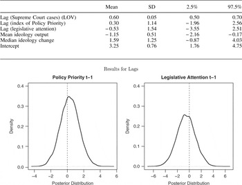
We implement this specification as a Bayesian linear regression and estimate it via MCMC (Gibbs sampling).Footnote ⁶ In this model, we also include a lagged outcome variable and fixed effects for policy area. The results in Table 1, which we consider the baseline results for the theoretical model,Footnote ⁷ are reported for a model with policy priority and legislative attention, each lagged one year. In this instance, the first-period lag on the primary regressor of interest—the policy priority index—reveals little evidence of systematic influence on the future number of Supreme Court cases. This is unsurprising, given the results of Baird (Baird Reference Baird2004; Baird Reference Baird2007) and Peters (Reference Przeworski and Limongi2007), where the significant impact came in later years though the exact time period was not known or specified a priori. It is this dynamic process and the impact of specification we hope to model below.

Table 1

The Baseline Litigant Signal Model

Note: N=435. The outcome variable in this analysis is the total number of Supreme Court cases within a policy area during a year. The specification includes a lagged outcome variable, and one-year lags on index for Policy Priority and the variable for Legislative Attention. Fixed effects for the Chief Justice and policy area were included but are not reported.

Distributed Lag Model

In previous examinations of the litigant signal model (Baird Reference Baird2004; Baird Reference Baird2007), Baird has utilized a distributed lag approach with six lags of two variables: indexes of the Court’s policy priorities and indexes of legislative attention. The model has therefore included six lags of the index of Supreme Court policy priorities and six lags of a measure of legislative attention, used as controls. Baird defines the feasible set, though the length of these lags is acknowledged as atheoretic: “I chose to include the first six lagged years of the index because it would be difficult to claim that the effect of the signal of policy priorities would last longer than six years” (Reference Baird2007, 94).

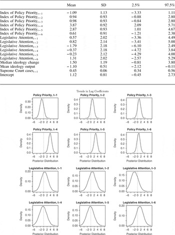
The results of our distributed lag model based on the theoretical model in Equation 1 and Baird’s (Reference Baird2004) specification of the feasible set are presented in Table 2. As before, dichotomous variables for each policy area and sitting Chief Justice are included in the model but are not reported here.

Table 2

Distributed Lag Linear Model of Supreme Court Caseloads

Note: N=387. The outcome variable in this analysis is the total number of Supreme Court cases within a policy area during a year. The specification includes distributed lags k={1, 2, … , 6} for Legislative Attention and the index of policy priorities. Controls for the Chief Justice and policy area were included but are not reported above.

The distributed lag analysis in Table 2 shows the strongest relationships at the fourth and fifth lags of the index of Policy Priority; not only are the posterior means greatest for these lags, but they are the only lags for which the 95 percent credible intervals do not include 0. We can draw no such conclusions from any of the lags of Legislative Attention. In the lower cell of the table, we present density plots of the posterior distributions of the index of Policy Priority and Legislative Attention. We can see yet more clearly that only four- and five-year lags for Policy Priority exhibit a marked relationship with subsequent Supreme Court attention.

The results in Table 2 providing evidence that four and five years after the Supreme Court indicates a policy area as a priority, there is a significant increase in the total number of cases the Court hears in that policy area. The only other effect on which we can draw any conclusion is the measure of the ideological output of the Court.

Why did this model not fit better or produce more in the way of clear results? With two variables each lagged six times as well as a lagged outcome variable, the model has a large amount of potential collinearity, which biases standard errors upwards and leads to type I errors. The inclusion of such a large number of collinear lagged variables also leads to overfit models, which may present problems for future refinements in litigant signal models of Supreme Court agenda setting. As but one example, the model includes no indication of Presidential agenda priorities, despite the fact that executive branch attention influences the attention of other institutions (Flemming, Wood and Bohte Reference Flemming, Dan Wood and Bohte1999) and—through the office of the solicitor general—exerts strong and consistent influence on the Court’s behavior (e.g., Nicholson and Collins Reference Peters2008).

BMA and Atheoretic Lags

We now adapt the specification of the litigant signal model from its distributed lag specification above in order to average across multiple models with varying lags. Such an approach better reflects our uncertainty over the appropriate lag length, while mitigating collinearity and avoiding overfit models. Recall that the two regressors for which we have atheoretic lag problems are the index of Policy Priority and the measure of Legislative Attention. Baird (Reference Baird2007, 94) argued that it did not make sense for these effects to take longer than six years to affect the outcome, but did not have a theoretical reason for selecting a particular lag. Given the strengths of BMA, we can include additional lags; as documented below, changing the choice of the number of lags has little substantive effect on the conclusions we draw. Therefore, we estimate eight different models with Policy Priority and Legislative Attention both lagged between one and eight years, then average across the model space. The results are shown in Table 3.

Table 3

Bayesian Model Averaging Across Feasible Set: Litigant Signal Model

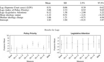
Note: N=387; feasible set=8. The outcome variable in this analysis is the total number of Supreme Court cases within a policy area during a year. The specification includes a lagged outcome variable, and atheoretic lags on index for Policy Priority and the variable for Legislative Attention. Fixed effects for the Chief Justice and policy area were included but are not reported.

Table 3 displays the posterior means of the lagged coefficients from the model averaging. Note first that the substantive results do not change from the distributed lag specification; only the index of Policy Priority and the measure of the Court’s ideological output have statistically reliable effects on future Supreme Court caseloads, as judged by their 95 percent credible intervals not including 0. In other words, the conclusions of the literature persist under our approach. Yet, the BMA approach does not lead to overconfident conclusions in particular time-series dynamics. Rather, in taking seriously the researcher’s a priori uncertainty over lag length, we conclude only that the amount of priority the Court accords some issue area has some subsequent influence on caseloads within that issue area.

This dynamic is particularly evident in the parameter plots of Table 3. Each plot in the Figure corresponds to one of the lagged regressors in the models. The points correspond to posterior means and the bars to 95 percent credible intervals across specifications. Take first the index of Policy Priority, where the posterior mean from model averaging (far right) is positive but with considerable associated uncertainty. This can be compared with the false negative identified in a baseline model (far left) and the six posterior means from the distributed lag model (middle). Although the researcher estimating distributed lag models without theory as to the lag length often engages in post-hoc justifications, there is no similar necessity under the BMA approach. Rather, the average posterior mean for the regressor of interest captures the effect as it relates to that variable without attempting to identify a particular lag length for which the researcher can only offer post-hoc justification.

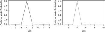
One potential concern of researchers considering using the BMA approach as compared with distributed lag models could be the loss of information as it relates to the length of the lagged effect, particularly where that may be of substantive interest to the scholar. Yet in those instances, BMA offers a further advantage. Rather than relying on estimates derived from models that are likely afflicted with the particular issues identified above, we can examine posterior model probabilities as derived in Equation 5, the precise entity with which some prior researchers have been concerned in proposing BMA (e.g., Montgomery and Nyhan Reference Montgomery and Nyhan2010). To that end, we plot the posterior model probabilities for each of the six estimated models in Figure 1. Note the high posterior model probability for the model featuring four-year lags of policy priority and legislative attention, consistent with prior work on the litigant signal model.

Fig. 1

Posterior model probabilities from Bayesian model averaging of litigant signal model Note: The left panel shows posterior model probabilities for the eighth-lag model. The right panel shows posterior model probabilities across different choices of the maximum number of lags. The probabilities line up so closely, that differences can only barely be distinguished at lags 4 and 5.

We turn now to demonstrating the robustness of the results across these alternatives, starting with the choice of the maximum lag length for the feasible set. Could the choice of the maximum lag length influence posterior model probabilities such that it biases any inference one may draw from the structure of the relationship? To test this, we estimate posterior model probabilities for maximum lags of four, six, eight, and ten periods and plot the results in the right panel of Figure 1. The lines are transparent gray, thus darker shades of gray indicate areas where the lines overlap. Such an approach is necessary as the lines are almost entirely overplotted; a function of the fact that there is little to no differentiation in posterior model probabilities across different selections of the maximum lag length.

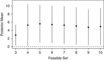
Similarly, one could be concerned that the choice of the maximum lag in the feasible set influences the BMA of the posterior means for the regressors. To examine this, in Figure 2 we plot the magnitude of the average posterior means of the regressor of interest, the index of Policy Priority, across choices of the maximum lag in the feasible set. Note that across choices of maximum lag lengths, posterior means are consistent with 95 percent credible intervals that do not include 0.

Fig. 2

Bayesian model averaged posterior means for index of Policy Priority across different specifications of maximum lag length Note: The plot shows the averaged posterior mean and 95 percent credible intervals for the index of Policy Priority across choices of the maximum lag in the feasible set.

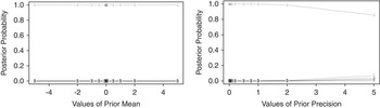
Finally, we examine the sensitivity of the results to the choice of prior mean and prior precision. In the left panel of Figure 3, we plot posterior model probabilities for each lag length across the choice of the prior mean.Footnote ⁸ Note that across specifications, the four-lag model retains the highest model probability. Similarly, in the right panel of Figure 3, we plot the posterior model probabilities, but across varying levels of prior precision. Of particular note is that, once again, across all possibilities considered, the posterior model probabilities consistently identify a four-lag model as best.

Fig. 3

Posterior model probabilities across choices of prior and prior precision Note: The left panel shows posterior model probabilities by lag for choices of the prior. The right panel shows posterior model probabilities by lag for choices of prior precision.

Thus, the results of BMA are broadly consistent with a distributed lag approach while avoiding the concomitant complications of distributed lag models. Moreover, in the undertheorized environment of atheoretic lags, BMA offers an approach that better reflects the uncertainty of the causal dynamics and, by virtue of averaging across a multitude of specifications, is less susceptible to the type of “p-hacking,” which recent research has identified as carrying broad implications for scientific studies (Gerber et al. Reference Gerber, Malhotra, Dowling and Doherty2010; Simonsohn, Nelson and Simmons Reference Tibshirani2014). We now move to a second application in order to demonstrate the broader utility of BMA to atheoretic lags in seemingly intractable research settings.

Application II: Modernization Theory

In the field of political economy, and at the intersection of comparative politics and international relations, modernization theory postulates a relationship between democracy and economic performance. Although modernization theory dates back to seminal works on economic modernization (Lerner Reference Lerner1958; Rostow Reference Simonsohn, Nelson and Simmons1960; Kuznets Reference Kuznets1966; Chenery and Taylor Reference Chenery and Taylor1968), the link between democratization and economic growth was first reported by Lipset (Reference Lipset1959). Lipset demonstrated a correlation between democracy and economic performance, and hypothesized that citizens become less tolerant of authoritarian regimes as they become more prosperous. Lipset’s results spurred the establishment of a substantial literature on the relationship between prosperity and democracy.

The literature on democratization is particularly robust in that it has examined the effects of economic growth using a wide variety of sampling frames. Large N statistical studies are common in this literature and yield consistent support for the importance of per capita GDP on the establishment and maintenance of democracy (Deutsch Reference Deutsch1961; Cutright Reference Cutright1963; Dahl Reference Dahl1971; Burkhart and Lewis-Beck Reference Burkhart and Lewis-Beck1994; Londregan and Poole Reference Londregan and Poole1996). Further, several well executed small N studies also find support for the effect of income on democratization (most notably Moore Reference Nicholson and Collins1966; Rueschemeyer, Stephens and Stephens Reference Solow1992).

An important contemporary contribution to this literature is a series of works by Adam Przeworski and colleagues (Prezeworski Reference Przeworski and Limongi1990; Przeworski and Limongi Reference Przeworski, Alvarez, Cheibub and Limongi1993; Przeworski et al. Reference Raftery1996; Przeworski and Limongi Reference Przeworski, Alvarez, Cheibub and Limongi1997) that culminated in the result that democracies seem to emerge at random, but that democratic endurance is correlated to income (Przeworski et al. Reference Rostow2000). Since the Przeworski et al. (Reference Rostow2000) result, the literature on democracy and income has progressed more slowly than before. Notable challenges to Przeworski and colleagues have come from Boix (Reference Boix2003), Boix and Stokes (Reference Boix and Stokes2003), and Epstein et al. (Reference Epstein, Bates, Goldstone, Kristensen and O’Halloran2006). Epstein et al. (Reference Epstein, Bates, Goldstone, Kristensen and O’Halloran2006) challenge Przeworski et al. (Reference Rostow2000) by using a trichotomous rather than dichotomous measure of democracy, thus capturing the difference between non-democracies, partial democracies, and full democracies. This slightly sharper coding scheme is perhaps more appropriate because the distribution of the Polity measure, on which the democracy codes are based, is severely bimodal. With their new outcome variable, Epstein et al. (Reference Epstein, Bates, Goldstone, Kristensen and O’Halloran2006) re-establish the effect of income on democracy.

As analyses of the relationship between income and democracy are generally conducted using panel data, it is possible that the reported results are either incomplete or non-robust because the atheoretic lag problems in these analyses have not been sufficiently addressed. Our goal is to re-examine the income–democracy relationship with special attention to the atheoretic lag problems. We do so in the context of slightly different data than such analyses have typically used. We look at the income–democracy relationship in the context of internal antagonisms that could inhibit the formation and perpetuation of democracy.

The data for this analysis are drawn from the study by Fearon and Latin (Reference Fearon and Latin2003) who have gathered a country-year data set covering the period 1945–99. The data include a number of variables expected to predict internal political stability and allow the post-war democracy–income relationship to be examined while controlling for precipitators of domestic instability.

We specify a theoretical model as follows:

(10) $$\eqalignno{ {\rm Democracy}\!=&\,{\rm Income}{\plus}{\rm Population} \cr & {\plus}{\rm Ethnic}\,{\rm Fract}{\rm .}{\plus}{\rm Religious}\, {\rm Fract}{\rm .} \cr & {\plus}{\rm Political}\,{\rm Instability} \cr & {\plus}{\rm Oil}{\plus}{\rm Non}\,{\minus}\,{\rm Contiguity}. $$

We use a dichotomous coding of democracy in which countries with Polity 2 scores <7 are coded as non-democracies, and countries with Polity 2 scores ≥7 are coded as democracies. The regressor of interest is income, measured as per capita GDP in the country-year. As controls for other sources of domestic stability/instability, we include measures for population, ethnic fractionalization, religious fractionalization, political instability, and indicators for whether the country produces oil and is non-contiguous. We use Fearon and Latin’s (Reference Fearon and Latin2003) coding and measures for all controls.

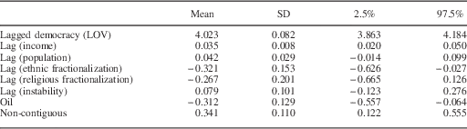
We implement the above specification as a Bayesian probit model of democracy (dichotomous scale) and the predictors described above, as well as a lagged outcome variable. Consider the results of the basic model, with the “default” one-period lags shown in Table 4. We see a small but significant effect for the one-period lag of income, significant negative effects for ethnic fractionalization, significant negative effects from oil exports, and evidence that non-contiguous states has a strong, significant, and positive effect on democracy. Each of these is consistent with our theory. However, the 95 percent credible intervals for the remainder of the variables contain 0, with log population, religious fractionalization, and political instability, all failing to attain results from which we can confidently draw any conclusions. This baseline model will serve as the jumping-off point for an exploration of this model’s atheoretic lag problem.

Table 4

The Baseline Modernization Theory Model

Note: N=6449. The specification lags the relevant regressors at the “default” value of one time period. The analysis includes a lagged outcome variable and year fixed effects (not reported).

Distributed Lag Model

Although the litigant signal model worked reasonably well as a distributed lag model, the modernization model does not. Here, beginning with a broad, inclusive model and testing restrictions—as (DeBoef and Keele Reference DeBoef and Keele2008) suggest—is impossible. Such a distributed lag model breaks down for the modernization application because of a larger feasible set, the need to estimate many parameters, and high autocorrelation in the variables for which we specify atheoretic lags.

We begin with consideration of the feasible set. The process of democratization is often a slow one. States are slow to change their governments and slow to react to the will of their people; this is particularly true with autocratic regimes (e.g., Cranmer and Siverson Reference Cranmer and Siverson2008). As we consider the regressors for which we have atheoretic lags (i.e., income, the log of population, ethnic fractionalization, religious fractionalization, and instability), we would not expect any of these variables to have particularly early effects on the democratic nature of a government. More likely, the effects of changes in these variables will take years to be observed. As such, we require a longer set of feasible lags than we had for the litigant signal model. In this case, we will specify a feasible set of lags ranging from one to ten years. Although this feasible set may seem a bit short, particularly for variables like population, if the regressors are indeed affecting the outcome, it seems reasonable to think that their effects would be apparent within the decade. That said, if our purpose was analytic rather than expository, a longer set of lags might well be used.

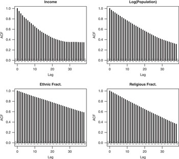
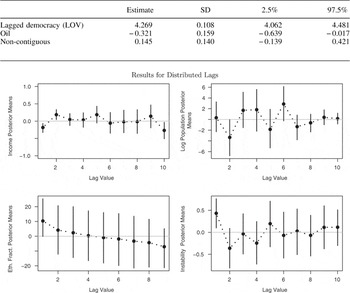
When we attempt to specify a distributed lag model based on the specification above and the atheoretic lags with ten-year feasible sets, we are quickly confronted with a problem. All but one of the parameters for the lags of religious fractionalization are not estimable. An examination of the autocorrelations for the variables with atheoretic lags in Figure 4 reveals the cause, including several lags of religious fractionalization results in such high collinearity in the model, that parameters are inestimable. Indeed, religious fractionalization is not the only variable about which we should be concerned.

Fig. 4

Autocorrelation functions (ACF) for four regressors in the modernization application for which atheoretic lags must be specified Note: Such high autocorrelations pose a problem for the estimation of distributed lag models.

The situation is not improved greatly if we are willing to drop religious fractionalization from our model; something an analysis for purposes other than exposition should not consider because the variable belongs in the model specification by theory. Nonetheless, if we are willing, for the purposes of exposition, to drop this variable entirely, we still have problems with estimation: high autocorrelations in ethnic fractionalization result in an inestimable parameter for its tenth lag. Furthermore, we know that high collinearity will still be present in the model because of the high autocorrelations of the remaining variables; even if the collinearity is not so high that the software is incapable of estimating parameters, such collinearity will bias uncertainty measures. The result of this poorly fitting specification can be seen in Table 5. Note that, according to this specification, income lagged one year is negatively related to democracy, whereas income lagged two years is positively related to democracy, both with credible intervals that do not contain 0. The same “switching” dynamic also appears with political instability and offers stark evidence of the ill effects of highly collinear specifications. Moreover, the posterior means and credible intervals of the non-continuous indicator no longer provides any evidence of a relationship with democracy. Finally, notice that the trends in the posterior means for the variables with distributed lags generally do not conform to either polynomial or exponential assumptions about their form, assumptions required for the distributed lag model.

Table 5

Distributed Lag Probit Results for Modernization Model

Note: N=5032. The outcome variable is democracy. Results for the regressors not specified as distributed lags are in the upper table, results for the distributed lags are presented graphically in the lower cell. The distributed lags are specified as k={1, 2, … , 10} for income, log of population, ethnic fractionalization, and instability. Note that a tenth lag for ethnic fractionalization could not be estimated due to collinearity.

In summary, following the standard advice of DeBoef and Keele (Reference DeBoef and Keele2008) is unworkable. We cannot estimate a distributed lag model with all the variables that theoretically ought to be in our model, a problem which is compounded by the fact that ten years is a short feasible set for this model but a longer feasible set is computationally impossible. One consequence of these problems are results that suggest peculiar dynamics. In all, the general distributed lag specification in the context of the modernization application is troublesome and illustrative of the limitations of this class of model.

Modernization Theory and BMA

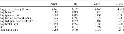
The advantages of BMA in the context of atheoretic lag problems are seen even more clearly here. Recall that we have five regressors with atheoretic lags such as income, instability, log of population, ethic fractionalization, and religious fractionalization. We also have a process for which we expect to have a longer feasible set of lags than was the case in the litigant signal model. In the above approach, the high degrees of collinearity prevented us from successfully modeling these data as distributed lags. Now, we specify a series of models that lags each of the atheoretic lag variables by up to 15 periods (more than was possible for the distributed lag model, even omitting the religious fractionalization variable), and compute posterior means of the lagged coefficients through model averaging. The results are shown in Table 6.

Table 6

Results of Bayesian Model Averaging Across Feasible Set

Note: N=6449; feasible set=15. The outcome variable in each of the analyses is democracy. For each of k={1, 2, … , 15}, the model is estimated, then we compute the Bayesian model averages for the coefficients from each of the 15 models.

Although the posterior means of the distributed lag were counter to expectations, the posterior means from BMA offer results that fit with the literature. First, results provide evidence that both non-lagged controls are significantly related to democracy. Second, in the case of the regressor of interest, we see that lagged income has a positive relationship with democracy, consistent with modernization theory. Third, the average posterior means and credible intervals for the other lagged variables provide evidence suggestive of theoretically intuitive patterns with credible intervals that do not include 0 for all but political instability. Finally, notice also that religious fractionalization, which could not even be included in the distributed lag specification, is now demonstrated to be negatively related with democracy.

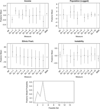
Figure 5 provides a comparison of the results from the several model approaches, which further reveals the advantage of BMA for atheoretic lag problems. We see that primary effect of interest, income, has a positive and significant effect. This is in keeping with the positive results from the baseline model but offers a clearer picture of the effect than the inconsistent “switching” result of the distributed lag model. Lagged values of log population have a significant and positive effect across models, a dynamic not identified at the first lag, and opposite to the significant and negative result seen at the first lag of the distributed lag model. Ethnic fractionalization and instability are never statistically significant at traditional thresholds, whereas a distributed lag model suggested that instability at one-year lags positively predicted predicts democracy. Finally, some may be concerned that the structure of the relationship at it relates to time is lost when using BMA. This, however, is not the case. The bottom panel of Figure 5 shows the posterior model probabilities (i.e., those from Equation 5) across the feasible set. We see that model probabilities peak at a four-year lag, and drop off quickly thereafter.

Fig. 5

Comparison of model results for modernization application Note: The outcome variable in each of the analyses is democracy. Each point represents the posterior mean of the coefficient, whereas the vertical bars represent 95 percent credible intervals. The lower panel presents posterior model probabilities across models estimated with each variable lagged k times, k={1, 2, … , 10} for the distributed lag (DL) application, and k={1, 2, … , 15} for the Bayesian model averaging (BMA) application.

We can see clearly in this application that BMA works particularly well for model specifications with atheoretic lags on many regressors and relatively long feasible lag sets. A researcher could gain further purchase on effects that differ over time (as opposed to just over lags) by creating subsets of the data for particular time periods of interest (i.e., during and after the Cold War) and re-running the multiple fit comparison analyses. See Cranmer and Siverson (Reference Cranmer and Siverson2008) for an example involving conflict pre- and post-WWII.

Concluding Thoughts

Social scientists frequently encounter research questions that feature temporal dynamics. To account for these dynamics, researchers include temporally lagged regressors in model specifications. Although in some cases the choice of the temporal lag is clear, in many instances there is no definitive a priori reason to suspect a particular lag or set of lags. We term these situations atheoretic lags, and have presented a set of techniques based on BMA to address the unique methodological concerns such situations invoke. These techniques, while based on the simple concept of averaging over repeated estimations across lags, appropriately account for model uncertainty in ways that common extant approaches do not. Moreover, our techniques overcome two prominent problems with one particularly common approach, distributed lag models: an excessively large number of regressors in a single model specification, and the introduction of high degrees of collinearity among the regressors.

We have shown, in the context of two examples in the discipline, the utility of the BMA approach across distributed lag specifications with atheoretic lags. Where the distributed lag specification works fairly well, as in the litigant signal model with only two variables with atheoretic lags and a feasible set of only six years, BMA recovers substantively identical results while mitigating concerns over the selective presentation of model specifications or p-hacking. Where the distributed lag approach breaks down, as in the modernization example with five atheoretic lag variables and a feasible set of 15 years, the BMA approach recovers estimates that accurately reflect the state of the world while avoiding the arbitrary selection of lag lengths or the omission of relevant variables. Therefore, we provide evidence that BMA offers an avenue by which scholars facing model specifications with atheoretic lags may reflect their underlying model uncertainty in a statistically rigorous way.

This simple solution comes with little cost, as the results are more easily presented than in distributed lag specifications, and the structure of the relationship across time can be recovered by examining posterior model probabilities. The relatively minor additional effort—estimating additional models—associated with this approach is one all too frequently incurred by researchers anyhow, though they then present only one specification. In sum, BMA offers researchers the means to gain and communicate substantive insight beyond what is possible with distributed lag models or the arbitrary choice of a particular lag length.