3.1. Chemical problem

To project (IIe) for the concentration at the surface of the particle onto a linear system, we expand the boundary fields

(3.2a,b)\begin{equation} c(\boldsymbol{b})=\sum_{q=0}^{\infty}w_{q}\boldsymbol{C}^{(q)}\odot\boldsymbol{Y}^{(q)}(\hat{\boldsymbol{b}}),\quad j^{\mathcal{A}}(\boldsymbol{b})=\sum_{q=0}^{\infty}\tilde{w}_{q}\boldsymbol{J}^{(q)} \odot\boldsymbol{Y}^{(q)}(\hat{\boldsymbol{b}}).\end{equation}

The product denoted by $\odot$ implies a maximal contraction of Cartesian indices (a $\boldsymbol {q}$-fold contraction between a tensor of rank-$q$ and another one of higher rank) and we have defined

(3.3a,b)\begin{equation} w_{q}=\frac{1}{q!\left(2q-1\right)!!},\quad\tilde{w}_{q}=\frac{2q+1}{4{\rm \pi} b^{2}}. \end{equation}

The expansion coefficients $\boldsymbol {C}^{(q)}$ and $\boldsymbol {J}^{(q)}$ are symmetric and traceless tensors of rank-$q$. The background concentration field $c^{\infty }(\boldsymbol {b})$ at the surface of the particle is expanded in an analogous manner to $c(\boldsymbol {b})$, with coefficients denoted by $\boldsymbol {C}^{\infty (q)}$. Linearity of the Laplace equation implies that the general solution in a basis of TSH can be written as

(3.4)\begin{equation} \boldsymbol{C}^{(q)}=\boldsymbol{\zeta}^{(q,q')}\odot\boldsymbol{C}^{\infty(q')}+\boldsymbol{\mathcal{E}}^{(q,q')}\odot\boldsymbol{J}^{(q')},\end{equation}

corresponding to (IIe), where the task now is to find the connecting tensors $\boldsymbol {\zeta }^{(q,q')}$ and $\boldsymbol {\mathcal {E}}^{(q,q')}$. In Appendix A, starting from the BIE for the surface concentration and using a Galerkin–Jacobi iterative method, we outline how to find approximate solutions, in leading powers of distance between the particle and surrounding boundaries, for these tensors in terms of a given Green's function $H$ of Laplace equation (Singh et al. Reference Singh, Adhikari and Cates2019).

Any Green's function $H$ of Laplace equation can be written as the sum

(3.5)\begin{equation} H(\boldsymbol{R},\tilde{\boldsymbol{R}})=H^{o}(\boldsymbol{r})+H^{*}(\boldsymbol{R},\tilde{\boldsymbol{R}}),\end{equation}

with $\boldsymbol {r}=\boldsymbol {R}-\tilde {\boldsymbol {R}}$, where $\boldsymbol {R}$ and $\tilde {\boldsymbol {R}}$ are the field and the source point, respectively. Here, $H^{o}(\boldsymbol {r})=1/4{\rm \pi} Dr$ is the fundamental solution of Laplace equation in an unbounded domain. On the other hand, $H^{*}$ is an extra contribution needed to satisfy additional boundary conditions in the system. For the unbounded case, where $H=H^{o}(\boldsymbol {r})$, the single-layer and double-layer operators in (IIb) and (IIc) have singular integral kernels. However, due to translational invariance they can be evaluated using Fourier techniques, see Appendix A.1. We find that both integral operators diagonalise simultaneously in a basis of TSH, yielding

(3.6a,b)\begin{equation} \boldsymbol{\zeta}^{(q,q')}=\zeta_{q}\,\boldsymbol{I}^{(q,q')},\quad \boldsymbol{\mathcal{E}}^{(q,q')}=\mathcal{E}_{q}\,\boldsymbol{I}^{(q,q')},\end{equation}

where

(3.7a,b)\begin{equation} \zeta_{q}=\frac{2q+1}{q+1},\quad\mathcal{E}_{q}=\frac{b}{D}\frac{\tilde{w}_{q}}{w_{q}}\frac{1}{q+1},\end{equation}

and $\boldsymbol {I}^{(q,q')}$ is a tensor with elements $\delta _{qq'}$, where the latter denotes a Kronecker delta. The expression for the elastance $\mathcal {E}_{q}$ is confirmed by previous results obtained by first solving the Laplace equation in the fluid volume and subsequently matching the boundary condition (Ic) for the surface flux (Jackson Reference Jackson1962; Golestanian et al. Reference Golestanian, Liverpool and Ajdari2007). If the system contains additional boundaries, we find corrections to these diagonal expressions in terms of derivatives of $H^{*}$. To leading order, this yields

(3.8)\begin{equation} \boldsymbol{\zeta}^{(q,q')}=\zeta_{q}\left(\boldsymbol{I}^{(q,q')}+4{\rm \pi} bDw_{q'}\frac{q'}{q'+1}b^{q+q'}\boldsymbol{\nabla}^{(q)} \tilde{\boldsymbol{\nabla}}^{(q')}H^{*}(\boldsymbol{R},\tilde{\boldsymbol{R}})\right),\end{equation}

where $\boldsymbol {\nabla }_{\alpha _{1}\dots \alpha _{q}}^{(q)}=\boldsymbol {\nabla }_{\alpha _{1}}\dots \boldsymbol {\nabla }_{\alpha _{q}}$, and where we have introduced the short-hand notation $\boldsymbol {\nabla }_{\boldsymbol {R}}=\boldsymbol {\nabla }$ for derivatives with respect to the field point and $\boldsymbol {\nabla }_{\tilde {\boldsymbol {R}}}=\tilde {\boldsymbol {\nabla }}$ for the source point. Similarly, we find for the elastance

(3.9)\begin{equation} \boldsymbol{\mathcal{E}}^{(q,q')}=\mathcal{E}_{q}\left(\boldsymbol{I}^{(q,q')}+4{\rm \pi} bDw_{q}\frac{2q'+1}{q'+1}b^{q+q'}\boldsymbol{\nabla}^{(q)}\tilde{\boldsymbol{\nabla}}^{(q')}H^{*} (\boldsymbol{R},\tilde{\boldsymbol{R}})\right).\end{equation}

In these expressions, the point of evaluation, $\boldsymbol {R}=\tilde {\boldsymbol {R}}$, for the one-body problem, is left implicit for brevity.

3.2. Hydrodynamic problem and Brownian motion

Using the linearity of Stokes flow we solve for the hydrodynamic traction $\boldsymbol {f}^{H}$ in a basis of TSH. Upon eliminating the hydrodynamic problem, Newton's equations (1.1a,b) will reveal the Brownian motion of an active particle. First, to find the linear system corresponding to (IIk), we expand the slip and the hydrodynamic traction in a basis of TSH

(3.10a,b)\begin{equation} \boldsymbol{v}^{\mathcal{A}}(\boldsymbol{b})=\sum_{l=1}^{\infty}w_{l-1}\boldsymbol{V}^{(l)}\odot\boldsymbol{Y}^{(l-1)}(\hat{\boldsymbol{b}}),\quad \boldsymbol{f}^{H}(\boldsymbol{b})=\sum_{l=1}^{\infty}\tilde{w}_{l-1}\boldsymbol{F}^{(l)}\odot\boldsymbol{Y}^{(l-1)}(\hat{\boldsymbol{b}}).\end{equation}

The coefficients $\boldsymbol {V}^{(l)}$ and $\boldsymbol {F}^{(l)}$ are rank-$l$ tensors, symmetric and traceless in their last $l-1$ indices. They can be decomposed into irreducible representations, denoted by $\boldsymbol {V}^{(l\sigma )}$ (or $\boldsymbol {F}^{(l\sigma )}$ for the traction moments), where $\boldsymbol {V}^{(ls)}$ (symmetric and traceless), $\boldsymbol {V}^{(la)}$ (anti-symmetric) and $\boldsymbol {V}^{(lt)}$ (trace) are irreducible tensors of ranks $l$, $l-1$ and $l-2$, respectively (Singh et al. Reference Singh, Ghose and Adhikari2015). For slip restricted by mass conservation only, obeying $\int \boldsymbol {v}^{\mathcal {A}}\boldsymbol {\cdot }\hat {\boldsymbol {b}}\,{\rm d}S=0$, these irreducible components of $\boldsymbol {V}^{(l)}$ (and $\boldsymbol {F}^{(l)}$) are independent of each other. In terms of the common definitions for the velocity and angular velocity of an active particle in an unbounded domain (Anderson & Prieve Reference Anderson and Prieve1991; Stone & Samuel Reference Stone and Samuel1996; Ghose & Adhikari Reference Ghose and Adhikari2014)

(3.11a,b)\begin{equation} \boldsymbol{V}^{\mathcal{A}}={-}\frac{1}{4{\rm \pi} b^{2}}\int\boldsymbol{v}^{\mathcal{A}}(\boldsymbol{b})\,{\rm d}S,\quad \boldsymbol{\varOmega}^{\mathcal{A}}={-}\frac{3}{8{\rm \pi} b^{3}}\int\hat{\boldsymbol{b}}\times\boldsymbol{v}^{\mathcal{A}} (\boldsymbol{b})\,{\rm d}S,\end{equation}

we have $\boldsymbol {V}^{(1s)}=-\boldsymbol {V}^{\mathcal {A}}$ and $\boldsymbol {V}^{(2a)}/2b=-\boldsymbol {\varOmega }^{\mathcal {A}}.$ Similarly, we have, for the hydrodynamic force and torque defined in (1.1a,b), $\boldsymbol {F}^{(1s)}=\boldsymbol {F}^{H}$ and $\boldsymbol {F}^{(2a)}=({1}/{b})\boldsymbol {T}^{H}$.

Linearity of the Stokes equation then allows us to write down the deterministic part of (IIk) in a basis of TSH

(3.12)\begin{equation} \boldsymbol{F}^{(l\sigma)} ={-}\boldsymbol{\gamma}^{(l\sigma,1s)}\boldsymbol{\cdot}\boldsymbol{V}-\boldsymbol{\gamma}^{(l\sigma,2a)} \boldsymbol{\cdot}\boldsymbol{\varOmega}-\hat{\boldsymbol{\gamma}}^{(l\sigma,l'\sigma')} \odot\boldsymbol{V}^{(l'\sigma')},\end{equation}

where $\boldsymbol {\gamma }^{(l\sigma,l'\sigma ')}$ and $\hat {\boldsymbol {\gamma }}^{(l\sigma,l'\sigma ')}$ are generalised friction tensors for rigid-body motion and slip, respectively. For the modes corresponding to rigid-body motion, it is known that $\boldsymbol {\gamma }^{(l\sigma,1s)}=\hat {\boldsymbol {\gamma }}^{(l\sigma,1s)}$ and $\boldsymbol {\gamma }^{(l\sigma,2a)}=\hat {\boldsymbol {\gamma }}^{(l\sigma,2a)}$ (Singh & Adhikari Reference Singh and Adhikari2018; Turk et al. Reference Turk, Singh and Adhikari2022). Therefore, we can write for the hydrodynamic force and torque

(3.13) \begin{multline} \begin{pmatrix}\boldsymbol{F}^{H}\\ \boldsymbol{T}^{H} \end{pmatrix}=-\boldsymbol{\varGamma}\boldsymbol{\cdot}\begin{pmatrix}\boldsymbol{V}-\boldsymbol{V}^{\mathcal{A}}\\ \boldsymbol{\varOmega}-\boldsymbol{\varOmega}^{\mathcal{A}} \end{pmatrix}-\sum_{l\sigma=2s}\hat{\boldsymbol{\varGamma}}^{(l\sigma)}\odot\boldsymbol{V}^{(l\sigma)},\\ \text{with}\quad\boldsymbol{\varGamma}=\begin{pmatrix}\boldsymbol{\gamma}^{TT} & \boldsymbol{\gamma}^{TR}\\ \boldsymbol{\gamma}^{RT} & \boldsymbol{\gamma}^{RR} \end{pmatrix},\quad\hat{\boldsymbol{\varGamma}}^{(l\sigma)}=\begin{pmatrix}\hat{\boldsymbol{\gamma}}^{(T,l\sigma)}\\ \hat{\boldsymbol{\gamma}}^{(R,l\sigma)} \end{pmatrix}\end{multline}

where the superscripts $T$ and $R$ imply $l\sigma =1s,2a$, respectively, to confirm with existing literature (Ladd Reference Ladd1988). The matrix $\boldsymbol {\varGamma }$ contains the friction on the particle due to rigid-body motion, and $\hat {\boldsymbol {\varGamma }}^{(l\sigma )}$ contains the friction due to higher modes of slip. This concludes the solution of the hydrodynamic problem without fluctuations.

In a thermally fluctuating fluid, the Brownian forces and torques obey the fluctuation–dissipation relations (Einstein Reference Einstein1905; Zwanzig Reference Zwanzig1964; Chow Reference Chow1973; Singh & Adhikari Reference Singh and Adhikari2017)

(3.14a,b)\begin{equation} \left\langle \begin{pmatrix}\hat{\boldsymbol{F}}(t)\\ \hat{\boldsymbol{T}}(t) \end{pmatrix}\right\rangle =\boldsymbol{0},\quad\left\langle \begin{pmatrix}\hat{\boldsymbol{F}}(t)\\ \hat{\boldsymbol{T}}(t) \end{pmatrix}\begin{pmatrix}\hat{\boldsymbol{F}}(t')\\ \hat{\boldsymbol{T}}(t') \end{pmatrix}^{\text{tr}}\right\rangle =2k_{B}T\,\boldsymbol{\varGamma}\,\delta(t-t'),\end{equation}

where angled brackets denote ensemble averages, $k_{B}$ is the Boltzmann constant and $T$ is the temperature, while the transpose is defined as $(A_{\alpha \beta })^{\textrm {tr}}=A_{\beta \alpha }$. Inserting the above equations for the deterministic and stochastic forces and torques into Newton's equations (1.1a,b) yields the Langevin equation

(3.15)\begin{align} \begin{pmatrix}m\dot{\boldsymbol{V}}\\ I\dot{\boldsymbol{\varOmega}} \end{pmatrix}=\begin{pmatrix}\boldsymbol{F}^{P}\\ \boldsymbol{T}^{P} \end{pmatrix}-\boldsymbol{\varGamma}\boldsymbol{\cdot}\begin{pmatrix}\boldsymbol{V}-\boldsymbol{V}^{\mathcal{A}}\\ \boldsymbol{\varOmega}-\boldsymbol{\varOmega}^{\mathcal{A}} \end{pmatrix}-\sum_{l\sigma=2s}\hat{\boldsymbol{\varGamma}}^{(l\sigma)}\odot\boldsymbol{V}^{(l\sigma)}+\sqrt{2k_{B}T\,\boldsymbol{\varGamma}} \boldsymbol{\cdot}\begin{pmatrix}\boldsymbol{\xi}^{T}\\ \boldsymbol{\xi}^{R} \end{pmatrix}.\end{align}

The parameters $\boldsymbol {\xi }^{\alpha }$ are random variables with zero mean and unit variance. In the inertial equation (3.15) the noise is not multiplicative since $\boldsymbol {\varGamma }$ is configuration dependent, but not velocity dependent. With the particle centre of mass $\boldsymbol {R}$ and its unit orientation vector $\boldsymbol {e}$ (its orientation is governed by the rotational dynamics $\dot {\boldsymbol {\varTheta }}=\boldsymbol {\varOmega }$, where $\boldsymbol {\varTheta }$ is an arbitrary set of angles), we can find its Brownian trajectory by integrating

(3.16a,b)\begin{equation} \dot{\boldsymbol{R}}=\boldsymbol{V},\quad\dot{\boldsymbol{e}}=\boldsymbol{\varOmega}\times\boldsymbol{e},\end{equation}

over time. In colloidal systems the inertia of both the particles and the fluid are typically negligible. This corresponds to the Smoluchowski limit of (3.15). Adiabatic elimination of the momentum variables in phase space then directly leads to the following update equations in Itô form (Ermak & McCammon Reference Ermak and McCammon1978; Gardiner Reference Gardiner1984; Wajnryb et al. Reference Wajnryb, Szymczak and Cichocki2004; Volpe & Wehr Reference Volpe and Wehr2016):

(3.17a) \begin{align} &\boldsymbol{R}(t+\Delta t) =\boldsymbol{R}(t)+\Delta\hat{\boldsymbol{R}}\nonumber\\ &\quad+\Big\{\boldsymbol{V}^{\mathcal{A}}+\boldsymbol{\mu}^{TT}\boldsymbol{\cdot}\boldsymbol{F}^{P}+\boldsymbol{\mu}^{TR}\boldsymbol{\cdot}\boldsymbol{T}^{P}+\sum_{l\sigma=2s}\boldsymbol{\rm \pi}^{(T,l\sigma)}\odot\boldsymbol{V}^{(l\sigma)}+k_{B}T\,\tilde{\boldsymbol{\nabla}}\boldsymbol{\cdot}\boldsymbol{\mu}^{TT}\Big\}\Delta t, \end{align}

(3.17b) \begin{align} &\boldsymbol{e}(t+\Delta t) =\boldsymbol{e}(t)+\Delta\hat{\boldsymbol{e}}\nonumber\\ &+\Big\{\boldsymbol{\varOmega}^{\mathcal{A}}+\boldsymbol{\mu}^{RT}\boldsymbol{\cdot}\boldsymbol{F}^{P}+\boldsymbol{\mu}^{RR}\boldsymbol{\cdot}\boldsymbol{T}^{P}+\sum_{l\sigma=2s}\boldsymbol{\rm \pi}^{(R,l\sigma)}\odot\boldsymbol{V}^{(l\sigma)}+k_{B}T\,\tilde{\boldsymbol{\nabla}}\boldsymbol{\cdot}\boldsymbol{\mu}^{RT}\Big\}\Delta t\times\boldsymbol{e}(t), \end{align}

with $\Delta \hat {\boldsymbol {e}}=\Delta \hat {\boldsymbol {\varTheta }}(t)\times \boldsymbol {e}(t)+\tfrac {1}{2} \Delta \hat {\boldsymbol {\varTheta }}(t)\boldsymbol {\cdot }[\boldsymbol {e}(t) \Delta \hat {\boldsymbol {\varTheta }}(t)-\Delta \hat {\boldsymbol {\varTheta }}(t)\boldsymbol {e}(t)]$, while

(3.18a,b)\begin{equation} \left\langle \begin{pmatrix}\Delta\hat{\boldsymbol{R}}\\ \Delta\hat{\boldsymbol{\varTheta}} \end{pmatrix}\right\rangle =\boldsymbol{0},\quad\left\langle \begin{pmatrix}\Delta\hat{\boldsymbol{R}}\\ \Delta\hat{\boldsymbol{\varTheta}} \end{pmatrix}\begin{pmatrix}\Delta\hat{\boldsymbol{R}}\\ \Delta\hat{\boldsymbol{\varTheta}} \end{pmatrix}^{\text{tr}}\right\rangle =2k_{B}T\,\mathbb{M}\,\Delta t.\end{equation}

It is clear that the grand mobility matrix $\mathbb {M}$ and the grand propulsion tensor $\boldsymbol {\varPi }^{(l\sigma )}$ satisfy

(3.19a,b)\begin{equation} \mathbb{M}=\begin{pmatrix}\boldsymbol{\mu}^{TT} & \boldsymbol{\mu}^{TR}\\ \boldsymbol{\mu}^{RT} & \boldsymbol{\mu}^{RR} \end{pmatrix}=\boldsymbol{\varGamma}^{{-}1},\quad\boldsymbol{\varPi}^{(l\sigma)}=\begin{pmatrix} \boldsymbol{\rm \pi}^{(T,l\sigma)}\\ \boldsymbol{\rm \pi}^{(R,l\sigma)} \end{pmatrix}={-}\mathbb{M}\boldsymbol{\cdot}\hat{\boldsymbol{\varGamma}}^{(l\sigma)}. \end{equation}

Onsager–Casimir symmetry implies symmetry of the mobility matrix, and we can identify the so-called propulsion tensors as $\boldsymbol {{\rm \pi} }^{(\alpha,l\sigma )}=-\boldsymbol {\mu }^{\alpha T}\boldsymbol {\cdot }\hat {\boldsymbol {\gamma }}^{(T,l\sigma )}-\boldsymbol {\mu }^{\alpha R}\boldsymbol {\cdot }\hat {\boldsymbol {\gamma }}^{(R,l\sigma )},$ with $\alpha \in \{T,R\}$ (Singh & Adhikari Reference Singh and Adhikari2018). The convective terms in the update equations constitute the thermal drift, which arises from a simple forward Euler integration scheme of the Langevin equations. The occurring derivative $\tilde {\boldsymbol {\nabla }}$ is the standard spatial gradient (with respect to the source point). If the mobilities depend on the particle orientation, additional orientational convective terms must be included. For the spherical particles considered here, however, these terms do not contribute. The quadratic term in $\Delta \boldsymbol {\varTheta }$ in $\Delta \hat {\boldsymbol {e}}$ is needed to preserve the condition $|\boldsymbol {e}|=1$, as discussed in Makino & Doi (Reference Makino and Doi2004) and De Corato et al. (Reference De Corato, Greco, D'Avino and Maffettone2015).

As the Stokes equation defines a dissipative system, any acceptable approximation of $\mathbb {M}$ must remain positive–definite for all physical configurations, e.g. when a simulated particle does not overlap with nearby boundaries (Cichocki et al. Reference Cichocki, Jones, Kutteh and Wajnryb2000). In Appendix B, starting from the BIE of Stokes flow and using a Galerkin–Jacobi iterative method, we outline how to find such solutions, in principle to arbitrary accuracy in the distance between the particle and surrounding boundaries, for the mobility and propulsion tensors in terms of the Green's function $\boldsymbol {G}$ of Stokes flow. For this, we write the Green's function as the sum (Smoluchowski Reference Smoluchowski1911)

(3.20)\begin{equation} \boldsymbol{G}(\boldsymbol{R},\tilde{\boldsymbol{R}})=\boldsymbol{G}^{o}(\boldsymbol{r})+\boldsymbol{G}^{*}(\boldsymbol{R},\tilde{\boldsymbol{R}}),\end{equation}

where $\boldsymbol {r}=\boldsymbol {R}-\tilde {\boldsymbol {R}}$, and $\boldsymbol {G}^{o}(\boldsymbol {r})=(\boldsymbol {I}+\hat {\boldsymbol {r}}\hat {\boldsymbol {r}})/8{\rm \pi} \eta r$ is the Oseen tensor for unbounded Stokes flow (Oseen Reference Oseen1927; Pozrikidis Reference Pozrikidis1992). The term $\boldsymbol {G}^{*}$ is the correction necessary to satisfy additional boundary conditions in the system. In the unbounded domain, where ${\boldsymbol {G}=\boldsymbol {G}^{o}(\boldsymbol {r})}$, the mobility matrix $\mathbb {M}$ diagonalises and the propulsion tensors vanish identically,

(3.21a–d)\begin{equation} \boldsymbol{\mu}^{TT}=\mu_{T}\,\boldsymbol{I},\quad\boldsymbol{\mu}^{R}=\mu_{R}\,\boldsymbol{I}, \quad\boldsymbol{\mu}^{TR}=\boldsymbol{\mu}^{RT}=\boldsymbol{0},\quad \boldsymbol{\rm \pi}^{(\alpha,l\sigma)}=\boldsymbol{0}. \end{equation}

Here, $\mu _{T}=(6{\rm \pi} \eta b)^{-1}$ and $\mu _{R}=(8{\rm \pi} \eta b^{3})^{-1}$ are the well-known mobility coefficients for translation and rotation of a sphere of radius $b$ in an unbounded fluid of viscosity $\eta$ (Stokes Reference Stokes1850). For a system containing additional boundaries, we obtain corrections to the above expressions in terms of derivatives of $\boldsymbol {G}^{*}$. As shown in the Appendix, to leading order in the Jacobi iteration the mobilities are

(3.22a–c)\begin{align} \boldsymbol{\mu}^{TT}=\mu_{T}\left(\boldsymbol{I}+6{\rm \pi}\eta b\,\mathcal{F}^{0}\tilde{\mathcal{F}}^{0}\boldsymbol{G}^{*}\right),\quad \boldsymbol{\mu}^{TR}=\tfrac{1}{2}\mathcal{F}^{0}\,\tilde{\boldsymbol{\nabla}}\times\boldsymbol{G}^{*}, \quad\boldsymbol{\mu}^{RR}=\mu_{R}\,\boldsymbol{I}+\tfrac{1}{2}\boldsymbol{\nabla}\times\boldsymbol{\mu}^{TR}, \end{align}

where we have defined the differential operators $\mathcal{F}^{l}=\big(1+b^{2}/(4l+6)\nabla^{2}\big)$ and $\tilde{\mathcal{F}}^{l}=\big(1+b^{2}/(4l+6)\tilde{\nabla}^{2}\big)$.

Governed by the particle's activity, we choose to retain the leading symmetric and polar modes of the slip. As demonstrated in the next section, this requires the following propulsion tensors:

(3.23a–c) \begin{align} \boldsymbol{\rm \pi}^{(T,2s)}=\tfrac{10{\rm \pi}\eta b^{2}}{3}\mathcal{F}^{0}\tilde{\mathcal{F}}^{1}\left[\tilde{\boldsymbol{\nabla}}\boldsymbol{G}^{*}\right.&\left.+(\tilde{\boldsymbol{\nabla}}\boldsymbol{G}^{*})^{\text{tr}}\right],\qquad\boldsymbol{\rm \pi}^{(T,3t)}=-\tfrac{2{\rm \pi}\eta b^{3}}{5}\mathcal{F}^{0}\tilde{\nabla}^{2}\boldsymbol{G}^{*},\nonumber\\[1em] &\boldsymbol{\rm \pi}^{(T,4t)}=-\tfrac{2{\rm \pi}\eta b^{4}}{63}\mathcal{F}^{0}\tilde{\boldsymbol{\nabla}}\tilde{\nabla}^{2}\boldsymbol{G}^{*},\end{align}

given to leading order in the Jacobi iteration. The structure of the problem implies that $\boldsymbol {{\rm \pi} }^{(R,l\sigma )}=\tfrac {1}{2}(\boldsymbol {\nabla }\times \boldsymbol {{\rm \pi} }^{(T,l\sigma )}).$ To the given order these have been first obtained in Singh & Adhikari (Reference Singh and Adhikari2018).

3.3. Chemo-hydrodynamic coupling and resulting propulsion

We now consider the boundary condition (IIl), coupling the hydrodynamic to the chemical problem. We observe that the differential operator $\boldsymbol {\chi }$ defined in (Ig) implies tangential slip such that $\hat {\boldsymbol {b}}\boldsymbol {\cdot }\boldsymbol {v}^{\mathcal {A}}=0$, i.e. chemical gradients at the surface of the particle can only drive tangential slip flows. Satisfying this condition, we write the tangential modes in the expansion of the slip in (3.10a,b) with a subscript $s$ as $\boldsymbol {V}_{s}^{(l\sigma )}$. In order to obey the tangential slip condition, the symmetric and trace modes of the slip expansion coefficients have to satisfy

(3.24)\begin{equation} \boldsymbol{V}_{s}^{([l+2]t)}={-}l(2l+3)\boldsymbol{V}_{s}^{(ls)}.\end{equation}

This means that, whenever a $\boldsymbol {V}_{s}^{(ls)}$ mode is generated, a $\boldsymbol {V}_{s}^{([l+2]t)}$ mode of strength given by (3.24) will be generated too. For the anti-symmetric modes $\boldsymbol {V}_{s}^{(la)}$ there is no such condition as they produce tangential slip flow by definition (Singh et al. Reference Singh, Ghose and Adhikari2015).

Finally, to express the boundary condition (Ig) in a basis of TSH, we expand the phoretic mobility as

(3.25)\begin{equation} \mu_{c}(\boldsymbol{b})=\sum_{q=0}^{\infty}\tilde{w}_{q}\boldsymbol{M}^{(q)}\odot\boldsymbol{Y}^{(q)}(\hat{\boldsymbol{b}}).\end{equation}

The coefficients $\boldsymbol {M}^{(q)}$ are symmetric and traceless tensors of rank-$q$. This yields the linear system corresponding to (IIl)

(3.26)\begin{equation} \boldsymbol{V}_{s}^{(l\sigma)} =\boldsymbol{\chi}^{(l\sigma,q)}\odot\boldsymbol{C}^{(q)}.\end{equation}

The coupling tensor $\boldsymbol {\chi }^{(l\sigma,q)}$ is given in Appendix A.3, and satisfies $\boldsymbol {\chi }^{(l\sigma,0)}=\boldsymbol {0}$, i.e. a uniform surface concentration does not induce slip.

In principle, any form of tangential slip can be generated by the chemo-hydrodynamic coupling in (3.26). Here, we only consider the leading polar ($\boldsymbol {V}_{s}^{(3t)}$), chiral ($\boldsymbol {V}_{s}^{(2a)}$) and symmetric ($\boldsymbol {V}_{s}^{(2s)}$) modes. Using (3.24), we can identify

(3.27a–c)\begin{equation} \boldsymbol{V}^{\mathcal{A}}={-}\boldsymbol{V}_{s}^{(1s)}=\tfrac{1}{5}\boldsymbol{V}_{s}^{(3t)},\quad 2b\boldsymbol{\varOmega}^{\mathcal{A}}={-}\boldsymbol{V}_{s}^{(2a)},\quad \boldsymbol{V}_{s}^{(2s)}={-}\tfrac{1}{14}\boldsymbol{V}_{s}^{(4t)}.\end{equation}

In the following, we therefore parametrise polar, chiral and symmetric slip by $\boldsymbol {V}^{\mathcal {A}}$, $\boldsymbol {\varOmega }^{\mathcal {A}}$ and $\boldsymbol {V}_{s}^{(2s)}$, respectively. With this, the propulsion terms in the update equations (3.17) are

(3.28)\begin{equation} \sum_{l\sigma=2s}\boldsymbol{\varPi}^{(l\sigma)}\odot\boldsymbol{V}^{(l\sigma)}=5\begin{pmatrix} \boldsymbol{\rm \pi}^{(T,3t)}\\ \boldsymbol{\rm \pi}^{(R,3t)} \end{pmatrix}\boldsymbol{\cdot}\boldsymbol{V}^{\mathcal{A}}+\begin{pmatrix}\boldsymbol{\rm \pi}^{(T,2s)}-14\boldsymbol{\rm \pi}^{(T,4t)}\\ \boldsymbol{\rm \pi}^{(R,2s)}-14\boldsymbol{\rm \pi}^{(R,4t)} \end{pmatrix}\boldsymbol{\colon}\boldsymbol{V}_{s}^{(2s)},\end{equation}

for an autophoretic particle, and (3.26) yields

(3.29a)$$\begin{gather} \boldsymbol{V}^{\mathcal{A}} ={-}\frac{1}{4{\rm \pi} b^{3}}\sum_{q=1}^{\infty}\left[\frac{q+1}{2q+1} \boldsymbol{M}^{(q-1)}-q(q+1)\boldsymbol{M}^{(q+1)}\right]\odot\boldsymbol{C}^{(q)}, \end{gather}$$

(3.29b)$$\begin{gather}\boldsymbol{\varOmega}^{\mathcal{A}} ={-}\frac{3}{8{\rm \pi} b^{4}}\sum_{q=1}^{\infty}q \boldsymbol{M}^{(q)}\times'\boldsymbol{C}^{(q)}, \end{gather}$$

(3.29c)$$\begin{gather}\boldsymbol{V}_{s}^{(2s)} =\frac{3}{4{\rm \pi} b^{3}}\sum_{q=1}^{\infty}\left[\frac{q+1}{4q^{2}-1} \boldsymbol{M}^{(q-2)}+\frac{3q}{2q+3}\boldsymbol{M}_{{sym}}^{(q)}-q(q+1)(q+2) \boldsymbol{M}^{(q+2)}\right]\odot\boldsymbol{C}^{(q)}. \end{gather}$$

For brevity, we have left the solution for $\boldsymbol {C}^{(q)}$ of (3.4) implicit. Here, we have defined a cross-product for irreducible tensors as $(\boldsymbol {M}^{(q)}\times '\boldsymbol {C}^{(q)}){}_{\alpha }=\epsilon _{\alpha \beta \gamma }M_{\beta ({\scriptscriptstyle Q-1})}^{(q)}C_{\gamma ({\scriptscriptstyle Q-1})}^{(q)}$ and a symmetric and traceless product contracting $(q-1)$ indices, $(\boldsymbol {M}_{{sym}}^{(q)}\odot \boldsymbol {C}^{(q)})_{\alpha \beta }=\varDelta _{\alpha \beta,\alpha '\beta '}^{(2)}M_{\alpha '({\scriptscriptstyle Q-1})}^{(q)}C_{\beta '({\scriptscriptstyle Q-1})}^{(q)}$, where we have used the short-hand notation $Q=\gamma _{1}\gamma _{2}\dots \gamma _{q}$ for Cartesian indices (Damour & Iyer Reference Damour and Iyer1991).

4.1. Programmed Brownian motion in the bulk

In the bulk, far away from boundaries, we can simplify (3.17). First, we non-dimensionalise the equations by rescaling velocities by the speed of a particle with constant phoretic mobility, namely $4{\rm \pi} b^{2}\,V=\mu _{c}J_{1}/D$. Angular velocities are rescaled by $V/b$. Renaming rescaled variables such that (3.16a,b) reads the same, we obtain

(4.2a,b)\begin{equation} \partial_{t}\boldsymbol{R}=\boldsymbol{V}^{\mathcal{A}}+\sqrt{2D_{T}}\,\boldsymbol{\xi}_{T}, \quad\partial_{t}\boldsymbol{e}=\left(\boldsymbol{\varOmega}^{\mathcal{A}}+\sqrt{2D_{R}}\, \boldsymbol{\xi}_{R}\right)\times\boldsymbol{e},\end{equation}

where for a spherical body in an unbounded fluid the translational diffusivity $D_{T}=\mathcal {B}/6$ and the rotational diffusivity $D_{R}=\mathcal {B}/8$ are isotropic and defined in terms of the Brown number

(4.3)\begin{equation} \mathcal{B}=\frac{k_{B}T}{{\rm \pi}\eta b^{2}V}, \end{equation}

the ratio of Brownian to hydrodynamic forces. Analogously, a particle Péclet number can be defined by ${Pe}=1/\mathcal {B}$ (Mozaffari et al. Reference Mozaffari, Sharifi-Mood, Koplik and Maldarelli2018). For a model including modes up to second order in both the phoretic mobility and the flux expansion, the velocity and angular velocity read

(4.4a)$$\begin{gather} \boldsymbol{V}^{\mathcal{A}} ={-}\boldsymbol{e}_{1}+3m_{2}\left[3\boldsymbol{p}_{2}\left(\boldsymbol{p}_{2} \boldsymbol{\cdot}\boldsymbol{e}_{1}\right)-\boldsymbol{e}_{1}\right]-6m_{1}j_{2} \left[3\boldsymbol{e}_{2}\left(\boldsymbol{e}_{2}\boldsymbol{\cdot}\boldsymbol{p}_{1}\right)- \boldsymbol{p}_{1}\right], \end{gather}$$

(4.4b)$$\begin{gather}\boldsymbol{\varOmega}^{\mathcal{A}} ={-}\tfrac{9}{4}m_{1} \left(\boldsymbol{p}_{1}\times\boldsymbol{e}_{1}\right)-270m_{2}j_{2}\left(\boldsymbol{p}_{2} \boldsymbol{\cdot}\boldsymbol{e}_{2}\right)\left(\boldsymbol{p}_{2}\times\boldsymbol{e}_{2}\right), \end{gather}$$

where $m_{i}=M_{i}/M_{0}$ and $j_{2}=J_{2}/J_{1}$. As will be convenient later, we define the angles $\boldsymbol {e}_{1}\boldsymbol {\cdot }\boldsymbol {p}_{i}=\cos \alpha _{i}$, $\boldsymbol {e}_{1}\boldsymbol {\cdot }\boldsymbol {e}_{2}=\cos \beta$ and $\boldsymbol {e}_{2}\boldsymbol {\cdot }\boldsymbol {p}_{2}=\cos \gamma$. Without loss of generality, we choose $\boldsymbol {e}_{1}$ as the orientation of the particle. This constitutes a minimal model capable of modelling the five distinct types of motion (Lisicki et al. Reference Lisicki, Reigh and Lauga2018): (i) pure translation, (ii) pure rotation (spinning), (iii) parallel rotation and translation, (iv) perpendicular rotation and translation (circular swimming) and (v) helical motion. In the following we briefly discuss particle designs for each type of motion and analyse how thermal noise affects the dynamics by computing the mean-squared displacement (MSD) $\left\langle \Delta\boldsymbol{}{r}^{2}(t)\right\rangle = \left\langle [\boldsymbol{r}(t)-\boldsymbol{r}(0)]^2\right\rangle$ of selected examples.

Pure translation is the simplest kind of motion and is achieved by choosing $m_{1}=m_{2}=j_{2}=0$. The update equations are those of an active Brownian particle (ABP) with swimming direction $-\boldsymbol {e}_{1}$

(4.5a)$$\begin{gather} \boldsymbol{R}(t+\Delta t) =\boldsymbol{R}(t)-\boldsymbol{e}_{1}\Delta t+\sqrt{2D_{T}}\Delta\boldsymbol{W}_{T}, \end{gather}$$

(4.5b)$$\begin{gather}\boldsymbol{e}_{1}(t+\Delta t) =\boldsymbol{e}_{1}(t)+\sqrt{2D_{R}}\Delta\boldsymbol{W}_{R}\times\boldsymbol{e}_{1}(t), \end{gather}$$

where $\Delta \boldsymbol {W}_{T}$ and $\Delta \boldsymbol {W}_{R}$ are increments of mutually independent Wiener processes (Gardiner Reference Gardiner1985). In figure 1(a), we show the simulated (markers) and theoretical (dashed lines) MSDs for such a particle at various temperatures. The MSD for an ABP is known exactly and is given by (Fodor & Marchetti Reference Fodor and Marchetti2018)

(4.6)\begin{equation} \left\langle \Delta\boldsymbol{r}^{2}(t)\right\rangle _{{tra}}=6\left(D_{T}+D_{A}\right)t+2(V\tau)^{2}\left({\rm e}^{{-}t/\tau}-1\right), \end{equation}

where $D_{A}=\mu _{T}V^{2}\tau /3$ is the active diffusion coefficient and $\tau ^{-1}=2D_{R}$ is the persistence time due to rotational noise. The persistence time indicates a transition from a ballistic to a diffusive dynamics, clearly visible in the figure. In the limit of zero temperature, i.e. $\mathcal {B}=0$, the MSD reduces to

(4.7)\begin{equation} \left\langle \Delta\boldsymbol{r}^{2}(t)\right\rangle _{{tra}}^{\mathcal{B}=0}=(Vt)^{2}, \end{equation}

as indicated in the figure.

Figure 1.

Mean-squared displacement of the programmed Brownian motion of an autophoretic particle. In panels (a–c) we compare the non-dimensionalised MSDs of translational, circular and helical swimming computed for Brownian simulations with their theoretical predictions (see the main text for the latter) at various temperatures characterised by a particle Péclet number ${Pe}$. We define ${Pe}=\infty$ (no noise), ${Pe}=100$ (moderate noise) and ${Pe}=10$ (strong noise) following Mozaffari et al. (Reference Mozaffari, Sharifi-Mood, Koplik and Maldarelli2018). For all three types of motion a diffusive regime ${\sim }t$ can be identified above a certain persistence time broadly determined by the amount of rotational diffusivity. The insets show the respective trajectories over an arbitrary time $T$ in the limit of zero temperature.

A spinning particle (pure rotation) can be modelled by choosing $\alpha _{2}={\rm \pi} /2$, $m_{2}=-1/3$ and $j_{2}=0$ while $\sin \alpha _{1}\neq 0$. This is captured by the update equations

(4.8a)$$\begin{gather} \boldsymbol{R}(t+\Delta t) =\boldsymbol{R}(t)+\sqrt{2D_{T}}\Delta\boldsymbol{W}_{T}, \end{gather}$$

(4.8b)$$\begin{gather}\boldsymbol{e}_{1}(t+\Delta t) =\boldsymbol{e}_{1}(t)+\tfrac{9}{4}m_{1}\left(\boldsymbol{p}_{1}(t)-\boldsymbol{e}_{1}(t) \cos\alpha_{1}\right)\Delta t+\sqrt{2D_{R}}\Delta\boldsymbol{W}_{R}\times\boldsymbol{e}_{1}(t). \end{gather}$$

Additional translation parallel to rotation, on the other hand, occurs for the parameter values $\alpha _{1}=0$, $\alpha _{2}=\beta ={\rm \pi} /2$ and $\sin (2\gamma )\neq 0$, with $\boldsymbol {e}_{1}$ as the translation and rotation axis of the update equations

(4.9a)$$\begin{gather} \boldsymbol{R}(t+\Delta t) =\boldsymbol{R}(t)-\boldsymbol{e}_{1}\left[1+3m_{2}-6m_{1}j_{2}\right]\Delta t+ \sqrt{2D_{T}}\Delta\boldsymbol{W}_{T}, \end{gather}$$

(4.9b)$$\begin{gather}\boldsymbol{e}_{1}(t+\Delta t) =\boldsymbol{e}_{1}(t)+\sqrt{2D_{R}}\Delta\boldsymbol{W}_{R}\times \boldsymbol{e}_{1}(t). \end{gather}$$

Circular swimming (perpendicular rotation and translation) is obtained by choosing $m_{2}=j_{2}=0$ and $\sin \alpha _{1}\neq 0$. For such a self-rotating circle swimmer one can compute the MSD exactly if the Brownian motion is confined to the plane perpendicular to $\boldsymbol {\varOmega }^{\mathcal {A}}$ (van Teeffelen & Löwen Reference van Teeffelen and Löwen2008)

(4.10)\begin{align} &\left\langle \Delta\boldsymbol{r}^{2}(t)\right\rangle _{{circ}}\nonumber\\ &\quad =2\lambda^{2}\left\{ \varOmega^{2}-D_{R}^{2}+D_{R}(D_{R}^{2}+\varOmega^{2})t+{\rm e}^{{-}D_{R}t}\left[(D_{R}^{2}-\varOmega^{2})\cos\varOmega t-2D_{R}\varOmega\sin\varOmega t\right]\right\}\nonumber\\ &\qquad +4D_{T}t, \end{align}

where $\lambda =V/(D_{R}^{2}+\varOmega ^{2})$. Here, $\varOmega$ represents the circular frequency. In the limit of zero temperature, this reduces to

(4.11)\begin{equation} \left\langle \Delta\boldsymbol{r}^{2}(t)\right\rangle _{{circ}}^{\mathcal{B}=0}=2\left(\frac{V}{\varOmega}\right)^{2}(1-\cos\varOmega t), \end{equation}

where $V/\varOmega$ is the radius of the circular motion. Since in this case we can restrict our attention to the $x$–$z$ plane, we can define the planar polar angle $\vartheta$ such that $\boldsymbol {e}_{1}=\cos \vartheta \,\hat {\boldsymbol {x}}+\sin \vartheta \,\hat {\boldsymbol {z}}.$ The update equations then take the simplified form

(4.12a)$$\begin{gather} x(t+\Delta t) =x(t)-\cos\vartheta\Delta t+\sqrt{2D_{T}}\Delta W_{x}, \end{gather}$$

(4.12b)$$\begin{gather}z(t+\Delta t) =z(t)-\sin\vartheta\Delta t+\sqrt{2D_{T}}\Delta W_{z}, \end{gather}$$

(4.12c)$$\begin{gather}\vartheta(t+\Delta t) =\vartheta(t)+\tfrac{9}{4}m_{1}\sin\alpha_{1}\Delta t+\sqrt{2D_{R}}\Delta W_{\vartheta}, \end{gather}$$

where $\Delta W_{x}$, $\Delta W_{z}$ and $\Delta W_{\vartheta }$ are increments of mutually independent Wiener processes. In figure 1(b) we compare the MSD obtained from simulations with the theoretical expressions.

Helical motion occurs for all other parameter values, representing a general non-axisymmetric phoretic particle. A simple example is given by choosing $j_{2}=0$ and $\cos \beta \neq 0$. The corresponding update equations are

(4.13a)$$\begin{gather} \boldsymbol{R}(t+\Delta t) =\boldsymbol{R}(t)+\left(9m_{2}\boldsymbol{p}_{2}\cos\beta-\boldsymbol{e}_{1} \left(1+3m_{2}\right)\right)\Delta t+\sqrt{2D_{T}}\Delta\boldsymbol{W}_{T}, \end{gather}$$

(4.13b)$$\begin{gather}\boldsymbol{e}_{1}(t+\Delta t) =\boldsymbol{e}_{1}(t)+\tfrac{9}{4}m_{1}\left(\boldsymbol{p}_{1}(t)- \boldsymbol{e}_{1}(t)\cos\alpha_{1}\right)\Delta t+\sqrt{2D_{R}}\Delta\boldsymbol{W}_{R}\times\boldsymbol{e}_{1}(t). \end{gather}$$

At zero temperature, the pitch angle $\psi$ of the resulting helix is given by the simple expression

(4.14)\begin{equation} \frac{\boldsymbol{V}^{\mathcal{A}}}{\left|\boldsymbol{V}^{\mathcal{A}}\right|}\boldsymbol{\cdot} \frac{\boldsymbol{\varOmega}^{\mathcal{A}}}{\left|\boldsymbol{\varOmega}^{\mathcal{A}}\right|}={-}\frac{9m_{2}\sin(2\beta)}{2\sqrt{1+m_{2}(6-\cos^{2}\beta)+3m_{2}^{2}(3-26\cos^{2}\beta)}}=\cos\psi. \end{equation}

In figure 1(c) we approximate the corresponding MSD by a superposition of translational and circular Brownian motion discussed in the previous paragraphs such that

(4.15)\begin{equation} \left\langle \Delta\boldsymbol{r}^{2}(t)\right\rangle _{{hel}}=\left\langle \Delta\boldsymbol{r}^{2}(t)\right\rangle _{{tra}}^{V_{{\perp}}}+\left\langle \Delta\boldsymbol{r}^{2}(t)\right\rangle _{{circ}}^{V_{{\parallel}}}-4D_{T}t, \end{equation}

where the last term is introduced to avoid accounting for translational noise twice. The superscripts of the MSD terms indicate which component of the velocity enters the respective terms. Here, $V_{\perp }$ is the component of the velocity perpendicular to the plane of the circular motion, and $V_{\parallel }$ the component within that plane. Naturally, in the limit of zero temperature this reduces to the exact deterministic MSD for a helix

(4.16)\begin{equation} \left\langle \Delta\boldsymbol{r}^{2}(t)\right\rangle_{{hel}}^{{det}}=(V_{{\perp}}t)^{2}+2\left(\frac{V_{{\parallel}}}{\varOmega} \right)^{2}(1-\cos\varOmega t). \end{equation}

There is good agreement between this approximation and the MSD computed from simulated Brownian trajectories. Compared with the MSD of an ABP in figure 1(a), a kink indicating the period $2{\rm \pi} /\varOmega$ of the circular part of the motion is clearly visible.

4.2. Autophoresis near a permeable interface

We now introduce a plane surface of two immiscible liquids of viscosity ratio $\lambda ^{f}=\eta _{2}/\eta _{1}$ and solute diffusivity ratio $\lambda ^{c}=D_{2}/D_{1}$ in the vicinity of the particle, see figure 2. The interface is characterised by the Green's functions in table 3. Here, $H$ satisfies the boundary condition of continuous normal flux $\hat {\boldsymbol {z}}\boldsymbol {\cdot }\boldsymbol {j}^{(1)}=\hat {\boldsymbol {z}} \boldsymbol {\cdot }\boldsymbol {j}^{(2)}$ across the interface, and $\boldsymbol {G}$ arises from the boundary conditions of continuous tangential flow $v_{\rho }^{(1)}=v_{\rho }^{(2)},$ vanishing normal flow $v_{z}^{(1)}=v_{z}^{(2)}=0$ and continuous tangential stress $\eta _{1}\sigma _{\rho z}^{(1)}=\eta _{2}\sigma _{\rho z}^{(2)}$ across the interface, where the index $\rho =x,y$ lies in the plane of the interface (Jones, Felderhof & Deutch Reference Jones, Felderhof and Deutch1975; Aderogba & Blake Reference Aderogba and Blake1978). The superscripts label whether the quantity of interest is above or below the interface, where $(1)$ refers to the positive half-space $z>0$.

Figure 2.

Half-coated phoretic particle near the surface of two immiscible liquids. Schematic representation of a half-coated phoretic particle (Janus particle) of radius $b$ and with orientation $\boldsymbol {e}_{1}$ at a height $h$ above an interface of viscosity ratio $\lambda ^{f}=\eta _{2}/\eta _{1}$ and diffusivity ratio $\lambda ^{c}=D_{2}/D_{1}$. The latter effectively measures how permeable the interface is to the solutes, where $\lambda ^{c}=0$ implies an impermeable and $\lambda ^{c}=1$ a perfectly permeable interface. Due to the cylindrical symmetry of the system we can restrict our attention to the $x$–$z$ plane, where the symbols $\parallel$ and $\perp$ imply motion parallel and perpendicular to the interface, respectively.

Table 3.

Green's functions for a plane interface. The Green's functions for the concentration (Laplace equation, left) and velocity (Stokes equation, right) fields near a plane, chemically permeable fluid–fluid interface of solute diffusivity ratio $\lambda ^{c}=D_{2}/D_{1}$ and viscosity ratio $\lambda ^{f}=\eta _{2}/\eta _{1}$ at $z=0$ are given. The particle is in the positive half-space $z>0$, where the solute diffusivity is $D_{1}$ and the fluid viscosity is $\eta _{1}$. We use $\boldsymbol {r}=\boldsymbol {R}-\tilde {\boldsymbol {R}}$ and $\boldsymbol {r}^{*}=\boldsymbol {R}-\tilde {\boldsymbol {R}}^{*}$, with the field point $\boldsymbol {R}=(x,y,z)^{\textrm {tr}}$ , the source point $\tilde {\boldsymbol {R}}=(\tilde {x},\tilde {y},\tilde {z})^{\textrm {tr}}$ and the relation $\tilde {\boldsymbol {R}}^{*}=\boldsymbol {\mathcal {M}}\boldsymbol {\cdot }\tilde {\boldsymbol {R}}$ between the physical position vector $\tilde {\boldsymbol {R}}$ and the position vector of the image singularities $\tilde {\boldsymbol {R}}^{*}$. The height of the centre of the particle above the interface is $\tilde {z}=h$. With this, we have $\tilde {\boldsymbol {R}}-\tilde {\boldsymbol {R}}^{*}=(0,0,2h)^{\textrm {tr}}.$ We define $\boldsymbol {\nabla }^{*}=\boldsymbol {\nabla }_{\boldsymbol {r}^{*}}$, $\mathcal {M}_{\beta \gamma }^{f}=(({1-\lambda ^{f}})/({1+\lambda ^{f}}))\delta _{\beta \rho }\delta _{\rho \gamma }-\delta _{\beta z}\delta _{z\gamma }$, the mirroring operator $\mathcal {M}_{\beta \gamma }=\delta _{\beta \rho }\delta _{\rho \gamma }-\delta _{\beta z}\delta _{z\gamma }$ and the index $\rho =x,y$ in the plane of the interface.

To discuss the chemo-hydrodynamic effect a plane interface has on autophoresis and Brownian motion, we choose a simple non-axisymmetric particle model. We truncate the expansions of the phoretic mobility and surface flux each at linear order and choose $J_{0}/3=J_{1}=J$, so that the particle has one inert pole ($j^{\mathcal {A}}=0$) and one active pole ($j^{\mathcal {A}}>0$ ($j^{\mathcal {A}}<0$) for $J>0$ ($J<0$), corresponding to a source (sink) of chemical reactants). This is a first-order approximation to a Janus swimmer so that for $J>0$ we have an inert-side-forward swimmer. We define $\boldsymbol {e}_{1}\boldsymbol {\cdot }\boldsymbol {p}_{1}=\cos \alpha$, where as before, $\boldsymbol {e}_{1}$ shall serve as the orientation of the particle. For $\sin \alpha \neq 0$ the particle is capable of phoretic self-rotation, see the discussion on circular swimming in the previous section.

We choose to truncate the generated concentration field at the surface of the particle at second order with the coefficients determined by (3.4). Since slip is proportional to gradients in the surface concentration we can ignore the terms $\boldsymbol {\zeta }^{(0,q)}$, $\boldsymbol {\zeta }^{(q,0)}$ and $\boldsymbol {\mathcal {E}}^{(0,q)}$. Cylindrical symmetry of the system can then be used to write the remaining non-zero chemical tensors in terms of scalar coefficients, which are given in table 4. For simplicity, we assume the absence of any background concentration field.

Table 4.

Chemical coefficients. Scalar coefficients for the linear response to a background concentration field and for the elastance tensors with $\varLambda ^{c}=(1-\lambda ^{c})/(1+\lambda ^{c})$, where $\lambda ^{c}=D_{2}/D_{1}$, and the height above the interface $\hat {h}=h/b$. We have used the exact unbounded coefficients in (3.6a,b) such that $\zeta _{1}=3/2$, $\mathcal {E}_{1}=3/8{\rm \pi} bD_{1}$ and $\mathcal {E}_{2}=5/2{\rm \pi} bD_{1}$. Cylindrical symmetry of the system implies, for the coupling to a linear background concentration field, $\boldsymbol {\zeta }^{(1,1)}=(\boldsymbol {I}-\hat {\boldsymbol {z}}\hat {\boldsymbol {z}})\,\zeta _{\parallel }^{(1,1)}+\hat {\boldsymbol {z}}\hat {\boldsymbol {z}}\, \zeta _{\perp }^{(1,1)}$. The relevant elastance tensors are $\boldsymbol {\mathcal {E}}^{(1,0)}=\hat {\boldsymbol {z}}\,\mathcal {E}^{(1,0)},$ $\boldsymbol {\mathcal {E}}^{(1,1)}=(\boldsymbol {I}-\hat {\boldsymbol {z}}\hat {\boldsymbol {z}})\, \mathcal {E}_{\parallel }^{(1,1)}+\hat {\boldsymbol {z}}\hat {\boldsymbol {z}}\,\mathcal {E}_{\perp }^{(1,1)},$ $\boldsymbol {\mathcal {E}}^{(2,0)}=-(3\hat {\boldsymbol {z}}\hat {\boldsymbol {z}}-\boldsymbol {I})\,\mathcal {E}^{(2,0)}$ and $\mathcal {E}_{\alpha \beta \gamma }^{(2,1)}=\mathcal {E}^{(2,1)}[(\delta _{\gamma \alpha }-\delta _{\gamma z}\delta _{\alpha z})\delta _{\beta z}+(\delta _{\gamma \beta }-\delta _{\gamma z}\delta _{\beta z})\delta _{\alpha z}+(3\delta _{\beta z}\delta _{\alpha z}-\delta _{\alpha \beta })\delta _{\gamma z}]$.

The induced slip sets the surrounding fluid in motion. The fluid then reacts back on the particle and causes rigid-body motion, governed by the equations of motion in (3.17), mediated by mobility and propulsion tensors. Again, the cylindrical symmetry of the system allows us to write the mobility and propulsion tensors in terms of scalar coefficients, summarised in table 5.

Table 5.

Hydrodynamic coefficients. Scalar coefficients for the mobility matrices and the relevant propulsion tensors with $\lambda ^{f}=\eta _{2}/\eta _{1}$ and the height above the interface $\hat {h}=h/b$. Cylindrical symmetry of the system allows us to write, for the translational mobilities, $\boldsymbol {\mu }^{TT}\!=(\boldsymbol {I}-\hat {\boldsymbol {z}}\hat {\boldsymbol {z}})\mu _{\parallel }^{TT}+ \hat {\boldsymbol {z}}\hat {\boldsymbol {z}}\mu _{\perp }^{TT}$ and $\boldsymbol {\mu }^{TR}\!=(\boldsymbol {\mu }^{RT})^{\textrm {tr}}\!=\mu ^{TR}\boldsymbol {\epsilon }\boldsymbol {\cdot }\hat {\boldsymbol {z}}$. The mobility $\boldsymbol {\mu }^{RR}$ has the same structure as $\boldsymbol {\mu }^{TT}$ with the corresponding coefficients $\mu _{\parallel }^{RR}$ and $\mu _{\perp }^{RR}$. The propulsion tensor for the leading symmetric slip mode is ${{\rm \pi} _{\alpha \beta \gamma }^{(T,2s)}}={\rm \pi} _{1}^{(T,2s)}[(\delta _{\gamma \alpha }-\delta _{\gamma z}\delta _{\alpha z})\delta _{\beta z}+(\delta _{\beta \alpha }-\delta _{\beta z}\delta _{\alpha z})\delta _{\gamma z}]+{\rm \pi} _{2}^{(T,2s)}(\delta _{\gamma \beta }-3\delta _{\gamma z}\delta _{\beta z})\delta _{\alpha z}$. The propulsion tensor $\boldsymbol {{\rm \pi} }^{(T,4t)}$ is of the same structure as $\boldsymbol {{\rm \pi} }^{(T,2s)}$ with the corresponding coefficients ${\rm \pi} _{1}^{(T,4t)}$ and ${\rm \pi} _{2}^{(T,4t)}$. Since $\boldsymbol {{\rm \pi} }^{(T,3t)}$ has the same structure as $\boldsymbol {\mu }^{TT}$, we adopt an analogous notation with ${\rm \pi} _{\parallel }^{(T,3t)}$ and ${\rm \pi} _{\perp }^{(T,3t)}$. For the propulsion tensors contributing to the particle's rotational dynamics we obtain ${\rm \pi} _{\alpha \beta \gamma }^{(R,2s)}={\rm \pi} ^{(R,2s)}(\delta _{\beta z}\epsilon _{z\gamma \alpha }+\delta _{\gamma z}\epsilon _{z\beta \alpha })$ and $\boldsymbol {{\rm \pi} }^{(R,3t)}={\rm \pi} ^{(R,3t)}\boldsymbol {\epsilon }\boldsymbol {\cdot }\hat {\boldsymbol {z}}$. The propulsion tensor $\boldsymbol {{\rm \pi} }^{(R,4t)}$ is of the same structure as $\boldsymbol {{\rm \pi} }^{(R,2s)}$ with the corresponding coefficient ${\rm \pi} ^{(R,4t)}$.

The full set of mobility coefficients for a wall, a free surface or, indeed, a fluid–fluid interface have been obtained in the literature to a high degree of accuracy (Brenner Reference Brenner1961; Goldman, Cox & Brenner Reference Goldman, Cox and Brenner1967; Felderhof Reference Felderhof1976; Lee, Chadwick & Leal Reference Lee, Chadwick and Leal1979; Lee & Leal Reference Lee and Leal1980; Perkins & Jones Reference Perkins and Jones1990, Reference Perkins and Jones1992). In Appendix C we show that, for the plane boundary, the diffusion terms $\propto \sqrt {2k_{B}T\,\mathbb {M}}$ in (3.17) take a particularly simple analytic form and that, with the coefficients given in table 5, this diffusion matrix is inherently positive–definite for all physical configurations. The propulsion tensors are a unique feature of active particles and have not been obtained in this form in the literature before.

Assuming there is no external torque rotating the particle out of plane, i.e. $\boldsymbol {T}^{P}\boldsymbol {\cdot }\hat {\boldsymbol {z}}\,{=}\,0$, we can once again restrict our attention to the $x$–$z$ plane for which we define the planar polar angle $\vartheta$ such that $\boldsymbol {e}_{1}=\cos \vartheta \,\hat {\boldsymbol {x}}+\sin \vartheta \,\hat {\boldsymbol {z}}$. Autophoretic particles in typical experiments are neither force nor torque free due to mismatches between particle and solvent densities and between gravitational and geometric centres (Drescher et al. Reference Drescher, Goldstein, Michel, Polin and Tuval2010; Ebbens & Howse Reference Ebbens and Howse2010; Palacci et al. Reference Palacci, Cottin-Bizonne, Ybert and Bocquet2010, Reference Palacci, Sacanna, Steinberg, Pine and Chaikin2013; Buttinoni et al. Reference Buttinoni, Bialké, Kümmel, Löwen, Bechinger and Speck2013). Since the resulting forces and torques become dominant, at long distances, over active contributions, it is crucial to include their effects in our analysis. In simulating (3.16a,b) we therefore assume a bottom-heavy Janus particle (the chemically active coating, blue in figures, is assumed to be slightly heavier than the inert side, white in figures). Therefore, we have to take into account gravity in negative $z$-direction and a gravitational torque given by

(4.17a,b)\begin{equation} \boldsymbol{F}^{P}={-}mg\hat{\boldsymbol{z}},\quad\boldsymbol{T}^{P}=\kappa(\hat{\boldsymbol{z}}\times \boldsymbol{e})=\kappa\cos\vartheta\,\hat{\boldsymbol{y}}, \end{equation}

with $m$ the buoyancy-corrected mass of the particle, $g$ the gravitational constant and $\kappa$ a constant parametrising bottom heaviness. Inserting this into the update equations (3.17) with $\boldsymbol {R}=(x,y,h)^{\textrm {tr}}$, where $h(t)$ is the height of the particle above the boundary, we can now simulate the time evolution of this bottom-heavy, non-axisymmetric phoretic particle. In figure 3 we show typical trajectories near a free surface (e.g. an air–water surface) and a fluid–fluid interface of $\lambda ^{f}=50$ (e.g. an oil–water interface). We probe the effect of the nearby boundary on the dynamics of the autophoretic particle by truncating the dynamical system in (3.16a,b) at various orders in $h^{-1}$ and comparing the results; see Appendix C for the truncated expressions.

Figure 3.

Chemo-hydrodynamic effects of a boundary. We compare typical trajectories of a bottom-heavy non-axisymmetric active particle (see the main text for the chosen particle specifications) near two types of chemically impermeable ($\lambda ^{c}=0$) liquid–liquid interfaces. In panels (a,b) the interface is chosen to be a free air–water surface ($\lambda ^{f}=0$) and a water–oil interface ($\lambda ^{f}\approx 50$), respectively. The temperature in these panels is zero and the starting point (orientation) of the particle is indicated by a grey disk (line). In the upper panels we compare the trajectories of the particle obtained to various orders in the inverse distance to the wall $h^{-1}$, thus gradually including more interactions with the wall. Here, ‘simulation’ refers to the full dynamical system at the accuracy obtained in this paper. The lower panels show the orientational evolution of the particle in the various approximations in a polar plot, parametrised by the angle $\vartheta$ and the distance to the starting point. There are two main features to be observed when comparing (a,b). First, the particle tends to stay further away from the water–oil interface when compared with the air–water surface. This is expected as the particle's mobility perpendicular to the interface will be reduced with increasing viscosity ratio, see table 5. Second, the approximations are better for higher viscosity ratios. Again, this can be understood intuitively when considering the example that fluid flows produced near a wall decay faster in the far field when compared with fluid flows produced near a free surface (Aderogba & Blake Reference Aderogba and Blake1978). The slower decay of the latter means that, to achieve the same quality of approximation as with interfaces of higher viscosity ratios, higher orders in $h^{-1}$ are necessary. Panel (c) shows the same system as in panel (b) but with a finite particle Péclet number of ${Pe}=100$, representing experimentally relevant noise levels. It is clear that the translational as well as the rotational diffusion is affected by the presence of the interface. Thermal diffusion also induces a net repulsive effect between the particle and the interface.

At order $h^{-1}$ only hydrodynamic interactions with the boundary due to the gravitational force manifest themselves. It is at the next order, $h^{-2}$, that the gravitational torque and active effects become apparent. The latter comprise hydrodynamic interactions from symmetric propulsion via $\boldsymbol {{\rm \pi} }^{(T,2s)}$ and a purely monopolar chemical interaction with the interface. At this order in the approximation, fore–aft symmetry breaking of the particle is no longer necessary for self-propulsion near a boundary; see Appendix C. An isotropic particle with uniform phoretic mobility $\mu _{c}$ and surface flux $j^{\mathcal {A}}$ will get repelled (attracted) to the interface depending on whether it is a source or sink of chemical reactants and depending on the diffusivity ratio $\lambda ^{c}$ of the interface, see § 4.3 for a detailed discussion. Furthermore, at this order in the approximation the thermal advective term in (3.17) proportional to $\boldsymbol {\nabla }\boldsymbol {\cdot }\mathbb {M}$ starts to affect the dynamics. It is worth noting that, at order $h^{-3}$, our analytical results match those obtained in Ibrahim & Liverpool (Reference Ibrahim and Liverpool2015), using a method of reflections, for a Janus particle of trivial phoretic mobility near an inert no-slip wall.

The system parameters in figure 3 are chosen as follows. The starting position of the particle is at a height $\hat {h}_{0}=h(t=0)/b=2$ and an angle $\vartheta _{0}=-3{\rm \pi} /4$ to the wall. For the surface flux of the particle we choose the dimensionless control parameter $j_{1}=J_{1}/J_{0}=1/3$, modelling a source particle. Its phoretic mobility distribution is specified by the dimensionless parameter $m_{1}=M_{1}/M_{0}=0.7$, implying a significant non-isotropy ($m_{1}=0$ specifies a trivial phoretic mobility). The angle between the axes of surface flux and phoretic mobility is chosen such that $\alpha ={\rm \pi} /2$. In figure 3(c) the Brown number is set to $\mathcal {B}\sim 10^{-2}$, roughly matching a set of experiments on Janus colloids (Jiang, Yoshinaga & Sano Reference Jiang, Yoshinaga and Sano2010; Palacci et al. Reference Palacci, Sacanna, Steinberg, Pine and Chaikin2013) with a bead size $b\sim 1\ \mathrm {\mu } \textrm {m}$ and speed $v_{s}\sim 10\ \mathrm {\mu } \textrm {m}\ \textrm {s}^{-1}$. The ratios of gravitational to active forces and torques are chosen such that $mg/F_{A}\sim 10^{-1}$ and $\kappa /T_{A}\sim 10^{-2}$, respectively. Finally, inertial effects decay on the time scale of momentum relaxation, typically $\tau _{T}=m/6{\rm \pi} \eta b$ and $\tau _{R}=I/8{\rm \pi} \eta b^{3}=m/20{\rm \pi} \eta b$ for translational and rotational effects, respectively. The time step $\Delta t$ in our simulation is chosen such that $\tau _{T}/\Delta t\sim 10^{-4}$ and $\tau _{R}/\Delta t\sim 10^{-4}$, ensuring that the Smoluchowski limit of the dynamics provides an appropriate description.

4.3. Hovering above a permeable interface

As mentioned in the previous section, if chemo-hydrodynamic particle–boundary interactions of order $h^{-2}$ and higher are considered, fore–aft symmetry breaking of the particle is no longer necessary for self-propulsion near a boundary. Indeed, self-propulsion of isotropic particles near a boundary has been observed in light-activated phoretic swimmers (Palacci et al. Reference Palacci, Sacanna, Steinberg, Pine and Chaikin2013). We therefore consider a particle that is an isotropic source of reactants ($\mu _{c}=\textrm {const.}>0, j^{\mathcal {A}}=\textrm {const.}>0$) and investigate how its dynamics is affected by the viscosity ratio $\lambda^f$ and the diffusivity ratio $\lambda^c$ of the nearby interface in the limit of zero temperature. The particle is assumed to be driven towards the interface due to gravity. With the rotational dynamics and the translational dynamics parallel to the plane vanishing by symmetry, the particle is expected to hover above the interface at a height that can be found by solving $\dot {h}=0$, where $\dot {h}$ is given in Appendix C. Rescaling heights by $b$, mobilities by $\mu _{T}$ and velocities by $\mu _{T}mg$ and renaming the thus non-dimensionalised variables such that they read the same, we obtain the hovering condition

(4.18)\begin{equation} 0={-}\mu_{{\perp}}^{TT}+\tfrac{1}{4}\varLambda^{c}\mathcal{A}_{G}\left[h^{{-}2}(1+5{\rm \pi}_{{\perp}}^{(T,3t)})-3h^{{-}3}({\rm \pi}_{2}^{(T,2s)}-14{\rm \pi}_{2}^{(T,4t)})\right].\end{equation}

Hovering is thus characterised by only one dimensionless number, $\mathcal {A}_{G}=\mu _{c}j^{\mathcal {A}}/D\mu _{T}mg$, defined as the ratio of the speed of a uniformly coated phoretic particle in a uniform concentration gradient $j^{\mathcal {A}}/D$, namely $\mu _{c}j^{\mathcal {A}}/D$, to the settling velocity under gravity $\mu _{T}mg$. This is a measure of activity.

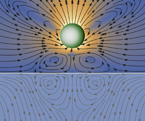
In figure 4, we show how in our approximation the hovering height $h$ of the isotropic particle is affected by its activity, the diffusivity ratio and the viscosity ratio of the boundary. We limit our results to $h>h_{{min}}=1.3$. This is because, very close to the interface, other effects such as electric double-layer and Van der Waals interactions are expected to dominate (Wu & Bevan Reference Wu and Bevan2005; Verweij et al. Reference Verweij, Ketzetzi, De Graaf and Kraft2020). As expected, a higher chemical diffusivity ratio of the interface, and thus decreased chemical repulsion from it, requires higher particle activities for hovering to remain possible; see figure 5 for an illustration of this effect using the method of images for the concentration field. It is also evident that lower levels of activity are sufficient for hovering above a free surface as compared with a solid wall. This is intuitive when considering that due to increased fluid internal friction flows near a wall decay faster than near a free surface (Aderogba & Blake Reference Aderogba and Blake1978) and so it is easier for a particle near a free surface to drive flows that make it hover. Using the method of images for Stokes flows this is illustrated in figure 6.

Figure 4.

Hovering above an interface. We show the hovering height $h$ (pseudo-colour map) for an active particle at zero temperature as a function of its activity $\mathcal {A}_{G}$ and the diffusivity ratio $\lambda ^{c}$ or the viscosity ratio $\lambda ^{f}$ of the interface. In panel (a) we consider the particle hovering above a wall ($\lambda ^{f}\rightarrow \infty$) that is permeable to the solutes. For a boundary between regions of equal solute diffusivity ($\lambda ^{c}=1$) there exists no chemical repulsion, leading to the particle inevitably crashing into the boundary. Therefore, we only consider values $\lambda ^{c} \, \leq 0.99$. The red line shows the particle's minimum activity to hover at a minimum height of $h_{{min}}=1.3$ as a function of the diffusivity ratio. The white region below the red line indicates physics that is not accessible in our simplified model and we assume that the particle crashes into the boundary due to gravity, i.e. we set $h=1$. The two dashed grey lines indicate the limiting values $\mathcal {A}_{G}^{1}\approx 500$ and $\mathcal {A}_{G}^{2}\approx 10^{5}$ that are required to hover above an impermeable and a highly permeable wall. In panel (b) we consider the particle hovering above an impermeable ($\lambda ^{c}=0$) interface of varying viscosity ratio. The two horizontal dashed grey lines indicate the limiting values $\mathcal {A}_{G}^{3}\approx 3$ and $\mathcal {A}_{G}^{1}$ that are required to hover above a free surface and a solid wall, respectively.

Figure 5.

Solute concentration for a particle hovering above a permeable boundary. The chemical field generated by a hovering source particle (green) is shown above ($z>0$) and below ($z<0$) the permeable ($\lambda ^{c}=0.3$) boundary as a pseudo-colour map, where contours indicate regions of constant concentration. We emphasise that the net concentration (right panel) in the region containing the particle is a superposition of the source without the boundary present (a) and its image below the boundary (b). The net concentration below the permeable boundary is then generated by the appropriate boundary conditions. To imply a change in the chemical diffusivity $D_{2}=\lambda ^{c}D_{1}$ the colour map for the region $z<0$ is shown with slightly reduced opacity. Since source particles want to move down chemical gradients (anti-chemotaxis), it is clear that the image creates a repulsive concentration field in $z>0$, making it possible for the particle to hover above the boundary. It is worth noting that, for an impermeable boundary ($\lambda ^{c}=0$), the contour lines meet the boundary at a right angle and the corresponding vector field ($\boldsymbol {\nabla }c$) becomes purely tangential to this ‘no-flux’ boundary. In the limit of rapid solute diffusion the viscosity ratio of the interface has no influence on the chemical field.

Figure 6.

Fluid flow for a particle hovering above a fluid–fluid interface. The fluid flow (laboratory frame) generated by a hovering source particle (green) is shown above ($z>0$) and below ($z<0$) a chemically permeable fluid–fluid interface ($\lambda ^{c}=0.3, \lambda ^{f}=10$). The direction of the fluid flow is indicated by black arrows, while its relative magnitude is implied by the overlaid pseudo-colour map. The net flow (c) in the region containing the particle is a superposition of the source without the boundary conditions on the fluid flow and stress (a) and its image below the boundary (b). Note that for the source the chemical boundary conditions must still be satisfied (see the net chemical field in figure 5), inducing a non-trivial slip on the otherwise isotropic particle. The net flow below the interface is then driven by the appropriate velocity and stress boundary conditions. To imply a change in the viscosity $\eta _{2}=\lambda ^{f}\eta _{1}$ the colour map for the region $z<0$ is shown with slightly reduced opacity. It is clear that the image produces an upwards flow in $z>0$ which balances gravity and makes the particle hover away from the interface. In the net flow this creates convection rolls between the particle and the interface which in turn drive convection rolls below the interface.